Abstract—This paper reports an evaluation of the performance of a Lee-Carter (LC) model which incorporated state space formulation (LC-SS model) in forecasting mortality rates. The parameters of the LC-SS model were estimated by maximum likelihood estimation (MLE) through an expectation-maximization (EM) algorithm. For this purpose, mortality data from Peninsular Malaysia for years 1980 to 2009 were used. The mortality data were split according to gender. Separate LC-SS models were each fitted for the male and female population. The performances of the LC-SS models were examined in terms of the accuracy of prediction based on in-sample fitting and out-of-sample forecasts. These performances were then compared with an original LC model estimated using the same data set. Comparisons were based on root mean square error (RMSE) and mean absolute percentage error (MAPE). The results indicate that the LC-SS model performs better than the original LC model.
Index Terms— Expectation-maximum algorithm, Lee-Carter model, mortality, state space model.
I. INTRODUCTION
ORTALITY rate is a determining factor of population growth. In the developed countries, the mortality rates have dropped, more or less continuously, since the start of the industrial revolution. Personal hygiene and improved sanitation have played a major role and preceded the impact of modern medicine and, in particular, the development of antibiotics capable of reducing death due to infection. The downward trend of the mortality rates is common to most countries, especially for developed countries and some of the developing countries. This change affects the population size and structure as well as national security. Hence, forecasts of mortality rates are important to areas such as demography, exclusively in population planning, social security, public health, policy making, directing pharmaceutical research, retirement and pension fund planning and life insurance. These beneficiaries benefit most from proper approach of forecasting mortality rates and have been attracting the interest of researchers in the last
Manuscript received March 06, 2015; revised March 30, 2015. This work was supported in part by the Ministry of Education, Malaysia and Universiti Teknologi MARA, Malaysia under SLAB scholarship.
W. H. W. Zakiyatussariroh is with the Faculty of Computer and Mathematical Sciences, Universiti Teknologi MARA, 40450 Shah Alam, Selangor, Malaysia (corresponding author: phone: +6019-3409511; fax: +603-55442000; e-mail: [email protected]).
M.S. Zainol, is with the Faculty of Computer and Mathematical Sciences, Universiti Teknologi MARA, 40450 Shah Alam, Selangor, Malaysia (e-mail: [email protected]).
M.R. Norazan is with the Faculty of Computer and Mathematical Sciences, Universiti Teknologi MARA, 40450 Shah Alam,Selangor, Malaysia (e-mail: [email protected]).
decade. Over the past century, various methods to forecast mortality have been introduced; such as in [1]-[4]. These methods were used by demographers and actuaries up to the early 1990s before they found that it underestimated the downward trend of mortality rates [5]. This underestimation problem occurred because time effects were not taken into consideration and the decreasing trend in mortality was ignored. Further, models were estimated for a specific time period only.
In 1992, a Lee-Carter (LC) model which considered the time effect in modeling and forecasting age-specific mortality was proposed [6]. Basically, the LC model involves a two-factor (age and time) model that is based on a log-bilinear form for age-specific mortality. The approach uses singular value decomposition (SVD) to extract a single time-varying mortality index which is then modeled as a time series, specifically, as random walk with drift. This has been seen as a significant milestone in demographic forecasting and has become the dominant approach used by actuaries, demographers and many other practitioners for forecasting age-specific mortality.
A number of approaches were developed with modifications and extensions of the LC model such as in [7]-[12]. These also included the reformulation of the LC model as state space model. As shown by [13]-[15], state space models are able to overcome most of the problems in the LC methodology. The main reason why a state space formulation of the LC model was suggested is due to the fact that errors of the LC equations were estimated separately. The first equation is estimated by a combination of singular value decomposition (SVD) while the second as a time series model. Reference [13] highlighted the fact that the prediction of the LC model only accounts for the error of time series model while ignoring the errors in estimating the parameters and the variance of the error term in the first equation. In state space formulation, all the parameters in the LC model were estimated simultaneously. There have been numerous efforts to reformulate the LC model as a state space by integrating the two equations of the LC model. State space formulation of the LC model, can be found in [13] and [16]. Reference [13] used Bayesian framework in estimating the Lee-Carter state space, henceforth, LC-SS and applied the model to the United States (US) mortality data, while, [16] used maximum likelihood estimation (MLE) through direct optimization algorithm. In addition, [17] was estimated the LC-SS parameters using MLE via expectation-maximization (EM) algorithm by applying it to Malaysian mortality data of total population. However, [17] only evaluated the LC-SS using in-sample fitting without forecasting and did not evaluate using out-sample forecasts.
Performance of the Lee-Carter State Space
Model in Forecasting Mortality
Wan Zakiyatussariroh Wan Husin, Mohammad Said Zainol and Norazan Mohamed Ramli
Thus, this study extends the work in [17] and evaluates the performance of LC-SS model on the Malaysian mortality data set, separated according to gender, with EM estimators.
II. METHODOLOGY
A. Lee-Carter Model
Let , the mortality rates for a group of ages in year
with = 1, … … , ( ) and = 1, … … . , ( ). LC model
actually analyzes the linear relationship between logarithm of original , and two factors that are age and year .
The model is presented as
, = + + , , (1)
where is the age pattern of log mortality rates averaged across year; is the first principal component reflecting relative change in the , at each age; is the first
set of principal score by year known as mortality index that measures the general level of the , and , is
the error term that assumed homoskedastic. The model was estimated using SVD with two constrains to ensure it is identifiable. The two constrains are ∑ = 0 and ∑ = 1.
In addition, the LC method adjusts by refitting it to the total number of deaths. The purpose of this adjustment is to give more weight to high rates [18]. The adjusted was then extrapolated using autoregressive integrated moving average (ARIMA) method [19],[20], specifically, ARIMA (0,1,0) as in the original paper of [6]. The ARIMA (0,1,0) is a random walk with drift model that is expressed as follow,
= + + = 1, … … , , (2) where is a drift parameter that measure the constant annual change in the series of and is the error terms. The procedures of LC method can be summarized as follow. 1) Estimating , and using historical age specific
mortality rates.
2) The estimated was adjusted to ensure equality between the observed and estimated number of deaths in a certain period.
3) The series of adjusted is then extrapolated as ARIMA.
4) Finally, the forecasted values of adjusted and the estimated and had substituted into (1) to get the forecasted values of ( ,). Then, convey back the
forecasted ( , ) to the original scale in order to get
forecast mortality rates. Thus, the ℎ-step forecast of
, is
, = exp + . (3)
B. State Space Lee-Carter Model
In order to overcome the weakness of the LC model in forecasting mortality, we employ LC-SS model. Let be the vector of N log mortality rates for year , =
( , , … , ) where is the value of the ith
mortality rates at time , ( = 1, … , and = 1, … , ). Thus, the LC-SS model can be expressed by
= + + with ~ ( , )
= + + with ~ (0, ), (4)
where = ( , , … , ), = ( , , … , ) and
= ( , , … , ) is a vector of error terms that are
assumed to be independent. A random walk with drift is assumed for the state vector. The error for the state is assumed to be independent and identically normally distributed with zero mean and constant variance q. The LC-SS model for the log mortality rates provides a joint distribution for the N age groups at any given time. It assumes that the observation noise is independent across time where are independent identically and normally distributed with × 1 variance vector, R. The errors and are uncorrelated. The unknown parameters in the model are denoted as = { , , , , , , } were estimated using MLE under the assumption that the initial state is normal that is ~ ( ,Σ ). The following is the joint log-likelihood function of the observations , , … . . ,
and the trend components , , … . . , ,
log ( , , … . . , , , , … . . , ) =
−1
2log( ) −
1
2 ( − )
−T
2log( )−
1
2 ( − − )
−T
2log| | + constant
−1
2 ( − − ) ( − − ).
This likelihood function is maximized numerically using the method of numerical maximizing, the EM algorithm as in [17] which was originally adopted from [21], [22]. It was maximized using the Kalman filter (KF) and smoother (KS). The EM algorithm involved the following steps [22], [23]. 1) Setting an initial estimates of parameters, .
On iteration j, (j = 0,1,2,…..):
2) Compute the incomplete-data likelihood and perform the E-Step. Based on initial parameters , the expected values of conditioned on all the observed data were calculated.
3) Perform the M-Step. A new set was computed by finding the parameters that maximize the expected log-likelihood function with respect to .
The overall procedures involved in EM were regarded as simply alternating between the KF and KS recursions. LC-SS forecasts the observables using KF recursion based on the MLEs that were obtained from the above recursive procedure.
III. DATA
The data sets used in this study is an all-cause mortality data for Malaysia. Mortality was measured by age-specific death rates (ASDR) provided by the Department of Statistics, Malaysia (DOSM). Data for Peninsular Malaysia for the period of 1980 to 2009 for both males and females were used. It consists of annual number of deaths and populations for 17 age groups which were organized into 5-year intervals; 0-4, 5-9, ..., 80+. Deaths with unknown age groups are not included in the analysis. The ASDR in a single calendar year were calculated as , = ,
, where
, is the number of deaths for a group of ages in year
and , is the observed population for a group of ages in
year . The observed population is estimated by taking a mid-year population for a group of ages. We used the years 1980 to 2005 to fit the models and do out-of-sample validation on the last 4 years.
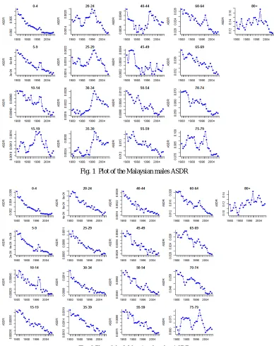
[image:3.595.108.496.288.778.2]Figure 1 and Fig. 2 respectively; show the ASDR over time for male population and female population for year 1980 to 2009. The ASDR fluctuated over this period. Mortality has decreased considerably in almost all age groups during the past 30 years and is much lower for females than for males. The decline in the female ASDR is steadier than those of the males. Notice that the male data appears much noisier than that for females. These data were then transformed to the logarithm (natural logarithm) due to the exponential nature in trend of ASDR. In addition, it is necessary to transform the raw data by taking logarithms in order to stabilize the high variance associated with high age-specific rates.
Fig. 1 Plot of the Malaysian males ASDR
IV. EMPIRICAL RESULTS
In this section, we report the forecasting ability of the LC-SS model compared to the LC model. Malaysian ASDR were fitted and forecasted separately for males and females using the two models. For the LC-SS model, following [23], the KF with initial mean 0 and variance 5 for initial setting of the state vector was used as in [17].
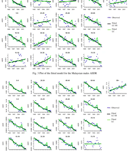
The results were first summarized by presenting the fitted values from both models compared to the original ASDR that were presented in Fig. 3 for male population and Fig. 4 for female population. Based on these values, the performance of the two models in fitting historical data was
[image:4.595.70.516.215.489.2]almost identical. It was also found that both models fit female data better than males. However, for certain age groups of males, both models were able to give good fit with the LC-SS performed better than the LC for age group 0-4, whereas, LC gives a good fit for age group 60-64. While, in the female case, both models performed well for all age groups except the 65-69 and 75-79 groups. Further, roughly, it can be seen that the LC-SS performed better than the LC in almost all of the age groups. These indicate that the estimated ASDR produced by both models vary. However, there does not appear to be a clear pattern of over or underestimation from these two models.
Fig. 3 Plot of the fitted model for the Malaysian males ASDR
Fig. 4 Plot of the Fitted models for the Malaysian females ASDR
Fitted LC-SS
Fitted LC Observed
Fitted LC-SS
[image:4.595.74.520.244.763.2]The models were then evaluated based on the goodness of fit for in-sample fitting and out-sample forecast of the ASDR. Commonly, in time series forecasting, the performance of in-sample fit is different from the out-of-sample fit. The better forecasting model is the one that performs well in out-of-sample fit [24]. Two different error measures were used; the root mean square error (RMSE) and mean absolute percentage error (MAPE). The performance evaluations of both models were carried out for each age group and overall performance for males and females respectively. In evaluating the performance according to each group, these measures of accuracy were averaged over years, whereas, for overall performance, these measures were averaged over different ages and years.
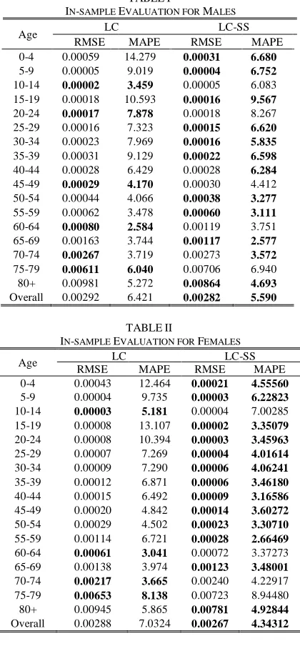
The results of the goodness of fit based on in-sample fitting respectively for both males and females are summarized in Table I and II. It is clear that the RMSE and MAPE for each age group for both males and females exhibit similar patterns.
TABLEI
IN-SAMPLE EVALUATION FOR MALES
Age LC LC-SS
RMSE MAPE RMSE MAPE 0-4 0.00059 14.279 0.00031 6.680
5-9 0.00005 9.019 0.00004 6.752
10-14 0.00002 3.459 0.00005 6.083 15-19 0.00018 10.593 0.00016 9.567
20-24 0.00017 7.878 0.00018 8.267 25-29 0.00016 7.323 0.00015 6.620
30-34 0.00023 7.969 0.00016 5.835
35-39 0.00031 9.129 0.00022 6.598
40-44 0.00028 6.429 0.00028 6.284
45-49 0.00029 4.170 0.00030 4.412 50-54 0.00044 4.066 0.00038 3.277
55-59 0.00062 3.478 0.00060 3.111
60-64 0.00080 2.584 0.00119 3.751 65-69 0.00163 3.744 0.00117 2.577
70-74 0.00267 3.719 0.00273 3.572
75-79 0.00611 6.040 0.00706 6.940 80+ 0.00981 5.272 0.00864 4.693
Overall 0.00292 6.421 0.00282 5.590
TABLEII
IN-SAMPLE EVALUATION FOR FEMALES
Age LC LC-SS
RMSE MAPE RMSE MAPE 0-4 0.00043 12.464 0.00021 4.55560
5-9 0.00004 9.735 0.00003 6.22823
10-14 0.00003 5.181 0.00004 7.00285 15-19 0.00008 13.107 0.00002 3.35079
20-24 0.00008 10.394 0.00003 3.45963
25-29 0.00007 7.269 0.00004 4.01614
30-34 0.00009 7.290 0.00006 4.06241
35-39 0.00012 6.871 0.00006 3.46180
40-44 0.00015 6.492 0.00009 3.16586
45-49 0.00020 4.842 0.00014 3.60272
50-54 0.00029 4.502 0.00023 3.30710
55-59 0.00114 6.721 0.00028 2.66469
60-64 0.00061 3.041 0.00072 3.37273 65-69 0.00138 3.974 0.00123 3.48001
70-74 0.00217 3.665 0.00240 4.22917 75-79 0.00653 8.138 0.00723 8.94480 80+ 0.00945 5.865 0.00781 4.92844
Overall 0.00288 7.0324 0.00267 4.34312
In males, both measures indicate that the error for the LC-SS model is smaller than the LC in almost all the age groups except for age groups 10-14, 20-24, 45-49, 60-64 and 75-79. In the case of females, the LC-SS performed better for most of the age groups with the LC-SS more dominant for the young and middle age groups, while, the LC performed well for the elderly age groups. However, if we refer to the overall performance, the LC-SS performed better than the LC for both males and females with the former having smaller values in both measures.
Similar results are obvious if we look at the overall performance of the models in out-sample prediction (Table III and Table IV) in which the LC-SS performed better than the LC for both males and females with both error measures of the LC-SS being smaller than of the LC. The same was evident if we look at the performance of the models for each of the age group for both males and females. A majority of the age groups show smaller values of RMSE and MAPE for the LC-SS model compared to the LC.
TABLE III
OUT-SAMPLE EVALUATION FOR MALES
Age LC LC-SS
RMSE MAPE RMSE MAPE 0-4 0.00096 51.480 0.00031 16.275
5-9 0.00008 27.167 0.00001 4.368
10-14 0.00006 13.448 0.00002 8.907
15-19 0.00040 37.581 0.00001 2.485
20-24 0.00039 29.488 0.00003 4.905
25-29 0.00048 31.761 0.00002 3.922
30-34 0.00052 23.814 0.00007 8.856
35-39 0.00048 17.273 0.00006 4.880
40-44 0.00008 1.7000 0.00009 5.350 45-49 0.00069 12.452 0.00012 3.724
50-54 0.00143 16.524 0.00017 2.638
55-59 0.00105 7.102 0.00018 2.092
60-64 0.00145 6.879 0.00071 5.954
65-69 0.00072 1.691 0.00236 11.381 70-74 0.00655 12.843 0.00217 5.129
75-79 0.00397 5.386 0.00775 12.228 80+ 0.03026 25.486 0.01737 14.262
Overall 0.00760 18.946 0.00707 6.903
TABLE IV
OUT-SAMPLE EVALUATION FOR FEMALES
Age LC LC-SS
RMSE MAPE RMSE MAPE 0-4 0.00060 37.837 0.00031 16.275
5-9 0.00005 22.331 0.00001 4.368
10-14 0.00002 6.795 0.00002 8.907 15-19 0.00003 8.620 0.00001 2.485
20-24 0.00005 10.200 0.00003 4.905
25-29 0.00007 12.853 0.00002 3.922
30-34 0.00016 21.331 0.00007 8.856
35-39 0.00015 13.307 0.00006 4.880
40-44 0.000251 14.879 0.00009 5.350
45-49 0.00031 10.720 0.00012 3.724
50-54 0.00050 10.443 0.00017 2.633
55-59 0.00041 5.240 0.00018 2.092
60-64 0.00047 3.852 0.00071 5.954 65-69 0.00120 5.795 0.00236 11.381 70-74 0.00137 3.030 0.00217 5.129 75-79 0.00820 12.940 0.00775 12.228
80+ 0.02276 18.835 0.01737 14.262
[image:5.595.64.274.290.742.2]V. CONCLUSION
We have modeled an extension of the LC model known as LC-SS model for forecasting mortality. Since the aim of this paper is to introduce an alternative approach to modeling and forecasting mortality rates, we did not compare the proposed approach with other competitive methods. Here, the performance of the LC-SS model was compared with the LC model only. Evaluations were carried out using in-sample and out-sample fit. Overall, it may be concluded that the LC-SS model fit Malaysian ASDR reasonably well for males and females in both evaluations with smaller errors measures compared to the LC model. Even though for certain age groups, the LC model produced estimated ASDR with lower error, it was found that the LC-SS model outperforms LC model for almost all age groups. Hence, for fitting the current data set, we can conclude that the performance of the LC-SS model is better than the LC model.
Further work for examining the LC-SS model with heterogeneous variance assumption for the age groups needs to be carried out. This extension should be considered because it is evident that in observed ASDR data, some age groups exhibit higher variability than others. Particularly, it was found in the elderly age groups which LC-SS model did not fit well with high variance are evident.
ACKNOWLEDGMENT
We thank the Department of Statistics Malaysia (DOSM) for the data. The authors are grateful to the Editor, the Associate Editor and anonymous referees for insightful comments and suggestions.
REFERENCES
[1] B. Gompertz, "On the Nature of the Function Expressive of the Law of Human Mortality, and on a New Mode of Determining the Value of Life Contingencies," Philosophical Transactions of the Royal Society of London, vol. 115, 1825, pp. 513-583.
[2] W. M. Makeham, "On the law of mortality," Journal of the Institute of Actuaries (1866), 1867,pp. 325-358.
[3] L. Heligman and J. H. Pollard, "The age pattern of mortality," Journal of the Institute of Actuaries, vol. 107, 1980, pp. 49-80.
[4] R. McNown and A. Rogers, "Forecasting mortality: A parameterized time series approach," Demography, vol. 26, 1989, pp. 645-660. [5] R. Mahmoudvand, F. Alehosseini, and M. Zokaei, "Feasibility of
Singular Spectrum Analysis in the Field of Forecasting Mortality Rate," Journal of Data Science, vol. 11, 2013, pp. 851-866.
[6] R. D. Lee and L. R. Carter, "Modeling and Forecasting U. S. Mortality," Journal of the American Statistical Association, vol. 87, 1992, pp. 659-671.
[7] N. Brouhns, M. Denuit, and J. K. Vermunt, "A Poisson log-bilinear regression approach to the construction of projected lifetables,"
Insurance: Mathematics and Economics, vol. 31, 2002, pp. 373-393. [8] A. J. G. Cairns, D. Blake, and K. Dowd, "A Two‐Factor Model for
Stochastic Mortality with Parameter Uncertainty: Theory and Calibration," Journal of Risk and Insurance, vol. 73, 2006, pp. 687-718.
[9] P. De Jong and L. Tickle, "Extending Lee–Carter Mortality Forecasting," Mathematical Population Studies, vol. 13, 2006, pp. 1-18.
[10] A. Delwarde, M. Denuit, and C. Partrat, "Negative binomial version of the Lee–Carter model for mortality forecasting," Applied Stochastic Models in Business and Industry, vol. 23, 2007, pp. 385-401. [11] R. J. Hyndman and M. Shahid Ullah, "Robust forecasting of mortality
and fertility rates: A functional data approach," Computational Statistics & Data Analysis, vol. 51, 2007, pp. 4942-4956. [12] D. Mitchell, P. L. Brockett, R. Mendoza-Arriaga, and K.
Muthuraman, "Modeling and Forecasting Mortality Rates," SSRN eLibrary, 2011.
[13] C. Pedroza, "A Bayesian forecasting model: predicting US male mortality," Biostatistics, vol. 7, 2006, pp. 530-550.
[14] F. Girosi, "Demographic forecasting," Ph.D. 3091567, Harvard University, United States -- Massachusetts, 2003.
[15] F. Girosi and G. King, Demographic forecasting: Princeton Univ Pr, 2008.
[16] D. Lazar and M. M. Denuit, "A multivariate time series approach to projected life tables," Applied Stochastic Models in Business and Industry, vol. 25, 2009, pp. 806-823.
[17] W. H. W. Zakiyatussariroh, M. S.Zainol, and M. R. Norazan, "Lee-Carter state space modeling: Application to the Malaysia mortality data," AIP Conference Proceedings, vol. 1602, 2014, pp. 1002-1008. [18] H. L. Shang, H. Booth, and R. J. Hyndman, "Point and interval
forecasts of mortality rates and life expectancy: A comparison of ten principal component methods," Demographic Research, vol. 25, 2011, pp. 173-214.
[19] J. D. Hamilton, Time series analysis vol. 2: Cambridge Univ Press, 1994.
[20] G. E. Box and G. Jenkins, "" Time Series Analysis for Forecasting and Control," Holden-D. iv, San Francisco, 1976.
[21] E. E. Holmes, E. J. Ward, and K. Wills, "Marss: Multivariate autoregressive state-space models for analyzing time-series data," The R Journal, vol. 4, 2012, pp. 11-19.
[22] R. H. Shumway and D. S. Stoffer, Time series analysis and its applications: with R examples: Springer, 2011.
[23] E. Holmes, E. Ward, and M. Scheuerell, "Analysis of multivariate time-series using the MARSS package," 2014