GAMA/
H-
ATLAS: The Local Dust Mass Function and
Cosmic Density as a Function of Galaxy Type - A
Benchmark for Models of Galaxy Evolution
R. A. Beeston
1
?
, A. H. Wright
2
,
3
, S. Maddox
1
,
4
, H.L. Gomez
1
, L. Dunne
1
,
4
,
S. P. Driver
2
, A. Robotham
2
, C. J. R. Clark
1
, K. Vinsen
2
, T. T. Takeuchi
5
,
G. Popping
6
,
7
, N. Bourne
8
, M. N. Bremer
9
, S. Phillipps
9
, A. J. Moffett
2
,
M. Baes
10
, J. Bland-Hawthorn
11
, S. Brough
12
, P. De Vis
13
, S. A. Eales
1
,
B. W. Holwerda
14
, J. Loveday
15
, J. Liske
16
, M. W. L. Smith
1
,
D. J. B. Smith
17
, E. Valiante
1
, C. Vlahakis
18
, L. Wang
19
,
20
1School of Physics & Astronomy, Cardiff University, Queens Buildings, The Parade, Cardiff , CF24 3AA, UK 2ICRAR, The University of Western Australia, 35 Stirling Highway, WA 6009, Australia
3Arglander-Institut f¨ur Astronomie, Universit¨at Bonn, Auf dem H¨ugel 71, 53121 Bonn, Germany
4SUPA. Institute for Astronomy, University of Edinburgh, Royal Observatory, Blackford Hill, Edinburgh, EH9 3HJ, UK 5Division of Particle and Astrophysical Science, Nagoya University, Furo-Cho, Chikusa-ku, Nagoya 464-8602, Japan 6European Southern Observatory, Karl-Schwarzschild-Strasse 2, 85748, Garching, Germany
7Max-Planck-Institut f¨ur Astronomie, K¨onigstuhl 17, D-69117 Heidelberg, Germany
8Institute for Astronomy, University of Edinburgh, Royal Observatory, Edinburgh EH9 3HJ, UK 9H. H. Wills Physics Laboratory, University of Bristol, Tyndall Avenue, Bristol BS8 1TL, UK 10Sterrenkundig Observatorium, Universiteit Gent, Krijgslaan 281 S9, B-9000 Gent, Belgium
11Sydney Institute for Astronomy, School of Physics, A28, The University of Sydney, NSW 2006, Australia 12School of Physics, University of New South Wales, NSW 2052, Australia
13Institut d’Astrophysique Spatiale, CNRS, Universit´e Paris-Sud, Universit´e Paris-Saclay, Bˆat. 121, 91405, Orsay Cedex, France 14Department of Physics and Astronomy, 102 Natural Science Building, University of Louisville, Louisville KY 40292, USA 15Astronomy Centre, University of Sussex, Falmer, Brighton BN1 9QH, UK
16Hamburger Sternwarte, Universit¨at Hamburg, Gojenbergsweg 112, D-21029 Hamburg, Germany
17Centre for Astrophyics Research, School of Physics, Astronomy and Mathematics, University of Hertfordshire, College Lane, Hatfield AL10 9AB, UK
18National Radio Astronomy Observatory, 520 Edgemont Road, Charlottesville, VA 22903, USA 19SRON Netherlands Institute for Space Research, Landleven 12, 9747 AD, Groningen, The Netherlands 20Kapteyn Astronomical Institute, University of Groningen, Postbus 800, 9700 AV, Groningen, The Netherlands
Accepted 2018 May 31. Received 2018 May 31; in original form 2017 December 12
ABSTRACT
We present the dust mass function (DMF) of 15,750 galaxies with redshiftz<0.1, drawn from the overlapping area of the GAMA and H-ATLAS surveys. The DMF is derived using the density correctedVmaxmethod, where we estimateVmaxusing: (i) the
normal photometric selection limit (pVmax) and (ii) a bivariate brightness distribution
(BBD) technique, which accounts for two selection effects. We fit the data with a Schechter function, and find M∗ = (4.65±0.18) ×107h270M, α = (−1.22±0.01),
φ∗ =(6.26±0.28) ×
10−3h703 Mpc−3dex−1. The resulting dust mass density parameter integrated down to104MisΩd=(1.11±0.02)×10−6which implies the mass fraction of
baryons in dust is fmb =(2.40±0.04)×10
−5; cosmic variance adds an extra 7-17 per cent
uncertainty to the quoted statistical errors. Our measurements have fewer galaxies with high dust mass than predicted by semi-analytic models. This is because the models include too much dust in high stellar mass galaxies. Conversely, our measurements find more galaxies with high dust mass than predicted by hydrodynamical cosmological simulations. This is likely to be from the long timescales for grain growth assumed in the models. We calculate DMFs split by galaxy type and find dust mass densities of
Ωd=(0.88±0.03) ×10−6 andΩd=(0.060±0.005) ×10−6 for late-types and early-types respectively. Comparing to the equivalent galaxy stellar mass functions (GSMF) we find that the DMF for late-types is well matched by the GMSF scaled by(8.07±0.35)×
10−4.
Key words: galaxies: statistics – galaxies: mass function – dust
?
©2018 The Authors
1 INTRODUCTION
Cosmic dust is a significant, albeit small, component of the interstellar medium (ISM) of galaxies. Despite being less than 1% of the baryonic mass of a galaxy, dust is responsi-ble for obscuring the ultraviolet and optical light from stars and active galactic nuclei and is thought to have absorbed approximately half of the starlight emitted since the Big Bang (Puget et al. 1996;Fixsen et al. 1998;Dole et al. 2006;
Driver et al. 2016). Measuring the dust mass in galaxies is therefore important for understanding obscured star forma-tion (Kennicutt 1998;Calzetti et al. 2007;Marchetti et al. 2016), particularly at different cosmic epochs (Madau et al. 1998;Hopkins 2004;Takeuchi et al. 2005). The dust mass function (DMF) is one of the fundamental measurements of the dust content of galaxies, providing crucial informa-tion on the reservoir of metals that are locked up in dust grains (Issa et al. 1990;Edmunds 2001;Dunne et al. 2003). A measure of the space density of dusty galaxies is becoming even more relevant given the widespread use of dust emis-sion as a tracer for the gas in recent years (Eales et al. 2010,
2012;Magdis et al. 2012;Scoville et al. 2014,2017; see also the comprehensive review of Casey et al. 2014). This is of particular interest given difficulties in observing atomic and molecular-line gas mass tracers out to higher redshifts ( Tac-coni et al. 2013;Catinella & Cortese 2015).
Ground-based studies including observations at 450 and 850µm with the Submillimetre Common User Bolometer Ar-ray (SCUBA) on the James Clerk Maxwell Telescope, led to the first measurements of the DMF over the mass range ∼107M < Md <few×108M (Dunne et al. 2000;Dunne
& Eales 2001;Vlahakis et al. 2005), whereMd is dust mass. Unfortunately the state-of-the-art at that time meant fewer than 200 nearby galaxies were observed with small fields of view and selected at optical or infrared (60µm) wavelengths. At higher redshifts, the Balloon-borne Large Aperture Sub-millimeter Telescope (BLAST, observing at 250-500µm) en-abled a DMF to be derived out to z=1(Eales et al. 2009) and a valiant effort to measure at even higher redshifts (z = 2.5) using SCUBA surveys was attempted by Dunne et al.(2003). These studies were hampered by small number statistics and difficulties with observing from the ground.
The advent of the Herschel Space Observatory (here-after Herschel, Pilbratt et al.(2010)) andPlanck Satellite revolutionised studies of dust in galaxies, as they enabled greater statistics, better sensitivity and angular resolution in some regimes, wider wavelength coverage and the ability to observe orders of magnitude larger areas of the sky than possible before. The largest dust mass function of galaxies usingHerschel was presented in Dunne et al. (2011) con-sisting of 1867 sources out to redshift z=0.5, selected from the Science Demonstration Phase (SDP) of theHerschel As-trophysical Terahertz Large Area Survey (H-ATLAS) blind 250-µm fields (Eales et al. 2010, 16 sq. degrees). Their DMF extended down to5×105Mand they derived a redshift de-pendent dust mass density ofΩd=ρd/ρcrit=(0.7−2) ×10−6. Subsequently, Negrello et al.(2013);Clemens et al.(2013) published the DMF of 234 local star-forming galaxies from the all sky Planck catalogue.Clark et al. (2015) then de-rived a local DMF from a 250-µm selected sample consist-ing of 42 sources. These DMFs ranged from106M<Md<
few×108M and 2×10⁵M < Md < 108M respectively.
These measurements1 were found to be consistent with the
z=0estimate fromDunne et al. (2011), once scaled to the same dust properties, as well as those derived from optical obscuration studies using the Milleniuum Galaxy Catalogue (Driver et al. 2007).
Interestingly, although the dust mass density is broadly consistent across most surveys, the shape of the dust mass function differs between all of these different estimates.
Clark et al.(2015) demonstrated using a blind survey se-lected at 250-µm, around a third of the dust mass in the local universe is contained within galaxies that are low stel-lar mass, gas-rich and have very blue optical colours. These galaxies were shown to have colder dust populations on av-erage (12<Td<16 K, whereTd is the cold-component dust temperature) compared to otherHerschel studies of nearby galaxies, e.g. theHerschel Reference Survey (Boselli et al. 2010), the Dwarf Galaxy Survey (Madden et al. 2013;R´ emy-Ruyer et al. 2013, see alsoDe Vis et al. 2017a) and higher stellar massH-ATLAS galaxiesSmith et al. (2012a). This led to higher numbers of galaxies in the low dust mass regime than predicted from extrapolating theDunne et al.(2011) DMF down to the equivalent mass bins (Clark et al. 2015). In comparison, theClemens et al.(2013) andVlahakis et al.(2005) DMFs are in reasonable agreement and both suggest a low-mass slope that is much steeper than the
Dunne et al.(2011) function. Overall, comparing between these different measures is complex due to different selec-tion effects; furthermore they are limited due to (i) small number statistics, and/or (ii) lack of sky coverage or vol-ume, inflating uncertainties due to cosmic variance. We also show evidence in Section4that fitting the same dataset over different mass ranges can have a significant effect on the re-sulting best-fit parameters. Since we probe further down the low-mass end than any literature study, this could therefore have a significant impact.
Here we further the study of the DMF by deriving the ‘local’ (z<0.1) dust mass function for the largest sample of galaxies to date, the sample is taken from the Galaxy and Mass Assembly Catalogue (GAMA,Driver et al. 2011). The large size of this sample reduces the statistical uncertainties and the effect of cosmic variance. We also employ statistical techniques to address selection effects in our sample, which allows us to probe further down the dust mass function by at least an order of magnitude compared to previous works. We present the observations and sample selection in Sec-tion2 and the method used to derive the dust masses for the GAMA sources in Section3. The dust mass function is presented in Section4and is compared to predictions from semi-analytical models in Section5. In Sections6and Sec-tion7, we split the DMF by morphological type and com-pare with their corresponding stellar mass functions, with conclusions in Section8. Properties of the full GAMA sam-ple are discussed in detail in Driver et al. (2017) and the accompanying stellar mass function of the same sample is published inWright et al.(2017), hereafter W17. Through-out this work we use a cosmology ofΩm=0.3,ΩΛ=0.7and
H0=70 km s−1Mpc−1.
2 OBSERVATIONS AND PHOTOMETRY
2.1 GAMA
The GAMA2survey is a panchromatic compilation of galax-ies built upon a highly complete magnitude limited spectro-scopic survey of around 286 square degrees of sky (with lim-iting magnituderpetro ≤19.8mag as measured by the Sloan Digital Sky Survey (SDSS) DR7, Abazajian et al. 2009). Around 238,000 objects have been successfully observed with the AAOmega Spectrograph on the Anglo-Australian Tele-scope as part of the GAMA survey. As well as spectrographic observations, GAMA has collated broad-band photometric measurements in up to 21 filters for each source from ul-traviolet (UV) to far-infrared (FIR)/submillimetre (submm) (Driver et al. 2016;Wright et al. 2017). The imaging data required to derive photometric measurements come from the compilation of many other surveys: GALEX Medium Imag-ing Survey (Bianchi & GALEX Team 1999); the SDSS DR7 (Abazajian et al. 2009), the VST Kilo-degree Survey (VST KiDS,de Jong et al. 2013); the VIsta Kilo- degree INfrared Galaxy survey (VIKING, de Jong et al. 2013); the Wide-field Infrared Survey Explorer (WISE,Wright et al. 2010); and the Herschel-ATLAS (Eales et al. 2010). The motiva-tion and science case for GAMA is detailed inDriver et al.
(2009). The GAMA input catalogue definition is described in
Baldry et al.(2010), and the tiling algorithm inRobotham et al.(2010). The data reduction and spectroscopic analy-sis can be found inHopkins et al.(2013). An overview and the survey procedures for the first data release (DR1) are presented in Driver et al. (2011). The second data release (DR2) was nearly twice the size of the first and is described inLiske et al.(2015). Information on data release 3 (DR3) can now be found in Baldry et al. (2018). There is now a vast wealth of data products available for the GAMA sur-vey, making it an incredibly powerful database for all kinds of extragalactic astronomy and cosmology.
K-corrections for GAMA sources are available from
Loveday et al. (2012) using k-correct v4 2 (Blanton &
Roweis 2007). Redshifts derived using autoz are available from Baldry et al.(2014). This work consists of data from the GAMA equatorial fields, which has a redshift complete-ness of >98 per cent at rpetro ≤19.8mag (Liske et al. 2015). GAMA distances were calculated using spectroscopic red-shifts and corrected (Baldry et al. 2012) to account for bulk deviations from the Hubble flow (Tonry et al. 2000).
For this paper, we select galaxies in the three equatorial fields of the GAMA survey, which cover∼180square degrees of sky between them. The equatorial fields G09, G12, G15 are located on the celestial equator at roughly 9 h, 12 h, and 15 h, respectively. We use the redshift range0.002≤z≤0.1, with the upper limit matching the low z bin from the ear-lier DMF study of Dunne et al.(2011); this redshift range contains 20,387 galaxies (with spectroscopic redshift quality set at nQual ≥ 3)3. These GAMA galaxies have been fur-ther split into Early Types (ETGs), Late Types (LTGs) and
2 http://www.gama-survey.org/
3 Here we use the following GAMA catalogues: LambdarCatv01, SersicCatSDSSv09, VisualMorphologyv03, DistancesFramesv14, and TilingCatv46 and themagphysresults presented in (Driver et al. 2017). We also removed one galaxy, GAMA CATAID 49167,
little blue spheroids (LBSs) based on classifications using giH-band images from SDSS (York et al. 2000), VIKING (Sutherland et al. 2015) or UKIDSS-LAS (seeKelvin et al. 2014;Moffett et al. 2016afor more details on the classifica-tion).
2.2 Herschel-ATLAS
The FIR and submm imaging data, which are necessary to derive dust masses, are provided viaH-ATLAS4 (Eales et al. 2010), the largest extragalactic Open Time survey using Herschel. This survey spans ∼660 square degrees of sky and consists of over 600 hours of observations in par-allel mode across five bands (100 and 160µm with PACS - Poglitsch et al. 2010, and 250, 350, and 500µm with SPIRE -Griffin et al. 2010).H-ATLAS was specifically de-signed to overlap with other large area surveys such as SDSS and GAMA. The GAMA/H-ATLAS overlap covers around 145 sq. degrees over the three equatorial GAMA fields, G09, G12, and G15. Photometry in the five bands for the
H-ATLAS DR1 is provided inValiante et al.(2016) based on sources selected initially at 250µm usingmadx(Maddox et al.in prep.) and havingS/N>4in any of the three SPIRE bands.Bourne et al.(2016) present optical counterparts to theH-ATLAS sources, identified from the GAMA catalogue using a likelihood ratio technique (Smith et al. 2011). In this paper, we use the aperture-matched photometry from Her-schelbased on the GAMAr-band aperture definitions using the LAMBDAR package (Wright et al. 2016), this method is described briefly in Section2.3.
Given the requirement forH-ATLAS and GAMA cover-age, the final sample for this work consists of 15,951 galaxies, this number includes a selection onrpetro≤19.8and the fact that due to the shapes of theH-ATLAS and GAMA fields, some of the GAMA sources were not covered byHerschel.
2.3 Photometry with LAMBDAR
The Lambda Adaptive Multi-band Deblending Algorithm in R (lambdar)5is an aperture photometry package developed byWright et al.(2016), which performs photometry based on an input catalogue of sources. Aperture-matched pho-tometry can be implemented on any number of bands and for each band the apertures are convolved by the PSF of the instrument. lambdar also deblends sources occupying the same on-sky area, this is achieved by sharing the flux in each pixel between all overlapping apertures. The frac-tional splitting is done iteratively and, depending on user preference, can be based on the mean surface brightness of a source, central pixel flux, or a user-defined weighting sys-tem. Each source is considered in a postage stamp of the in-put image focused on the source, the size of which depends upon the size of the aperture itself. All known sources within the postage stamp are deblended, including an optional list
due to an error in ther-band aperture chosen to derive the pho-tometry of this source.
4 http://www.h-atlas.org/ 5
lambdaris available from
of known contaminants specified by the user. For this pa-per this includesH-ATLAS detected sources fromValiante et al. (2016) which do not have a reliable optical counter-part. These are assumed to be higher redshift background sources.
The sky estimate for each source is calculated by ran-domly placing blank apertures with dimensions equal to the object aperture on the postage stamp, using the number of masked pixels in each blank aperture to weight its contribu-tion to the background estimate. Furthermore, during flux iteration, if any component of a blend is assigned a negative flux then it is rejected for all subsequent iterations (and any negative measurement is set to zero). There are a very small number of sources which end up with negative fluxes at the final iteration and, for consistency, the lambdar pipeline sets these to zero also. For the purposes of this work, we note that the fluxes for 11,210 (70.3 per cent) sources are not above the 3σ level at 250µm; however, even galaxies which fall below3σdo have a valid measurement and error estimate in five Herschel bands and thus provide informa-tion for deriving dust masses. We discuss potential biases and tests in later Sections. For further details on the lamb-darsoftware and data release seeWright et al.(2016).
3 DERIVING GALAXY PROPERTIES WITH
MAGPHYS
For each galaxy we take the dust and stellar properties from
Driver et al. (2017), who used the magphys6 package (da Cunha et al. 2008) to fit model spectral energy distributions (SEDs) to the 21-bandlambdarphotometry.magphysuses libraries containing 50 000 of model SEDs covering both the UV-NIR (Bruzual & Charlot 2003) and MIR/FIR ( Char-lot & Fall 2000) components of a galaxy’s SED along with a χ-squared minimisation technique to determine physical properties of a galaxy, including stellar mass, dust mass and dust temperature.magphysimposes energy balance be-tween these components, so that the power absorbed from the UV-NIR matches the power re-radiated in the MIR/FIR. In the FIR-submm regime, two major dust components are included in the libraries: a warm component (30 to 60 K) associated with stellar birth clouds; and a cold dust com-ponent (15 K to 25 K) associated with the diffuse ISM. A dust mass absorption coefficient ofκ850=0.077 m2kg−1is as-sumed, with an emissivity index ofβ=1.5for the warm dust, and β=2for cold dust, where κλ ∝λ−β. This is consistent with theκvalues derived from observations of nearby galax-ies (James et al. 2002;Clark et al. 2016, see alsoDunne et al. 2000) and∼2.4 times higher than the oft-usedDraine(2003) theoretical values (based on their κ scaled to 850µm with β=2)7. Using the latest values forκin the diffuse ISM of the Milky Way fromPlanck Collaboration XXIX(2016) would
6
magphysis available from http://www.iap.fr/magphys/ 7 We note that we have not considered the effects of changes in the dust mass absorption coefficientκin the different galaxy samples. As we are not able to test this using this dataset, we keep
κconstant in this work. Different grain properties could plausibly lead to an uncertainty of a factor of a few in κ (and therefore dust mass which scales withκ, see for example the discussion in Rowlands et al. 2014).
give dust masses 1.6 times higher than quoted here. For each galaxymagphysuses all of thelambdarmeasurements to find the best-fitting combination of optical and FIR model SEDs, and outputs the physical parameters for this com-bined SED. We do not apply any signal to noise cuts, but low signal to noise measurements clearly do not contribute strong constraints in the fitting. So long as the estimated fluxes and uncertainties are unbiased, this makes maximum use of the information available. magphys also generates a ‘probability distribution function’ (PDF) for each param-eter by summinge−χ2/2 over all models. The PDF for each parameter is used to determine the acceptable range of the physical quantity, expressed as percentiles of the probability distribution of model values. The results frommagphysfor the GAMA equatorial regions are presented inDriver et al.
(2016), and we use them throughout this work. For our anal-ysis we use the median value for each parameter, because this is more robust than the estimate from the best fit model combination. Where uncertainties are required, we use the
16th and84th percentiles, which correspond to a 1σ uncer-tainty for a Gaussian error distribution.
Our version ofmagphysis slightly modified compared to the default distribution available online. We use the most up-to-date estimates of theHerschel band-pass profiles for both the PACS and SPIRE instruments. Also in our version, the model photometry for each of theHerschelpass bands is calibrated to the nominal central wavelength of each band, as described in the SPIRE Handbook8 (Griffin et al. 2010,
2013), rather than the effective wavelength, which is the case for other photometry. Running the code with and without these changes does not highlight any systematic error in the FIR-basedmagphysoutput; however, it does change indi-vidual measurements by up to a few percent.
A large fraction of the GAMA sources have measure-ments with signal-to-noise ratio below3σin the FIR bands: for thez<0.1sample that we use here 32 per cent have fluxes >3σ. Given thatlambdarassigns a zero flux for each blend component that returns a negative flux at any iteration, the error distribution of faint sources becomes one-sided. If we assume that the errors are Gaussian and consider sources which have a true flux much less thanσ, then the bias in-troduced is the mean value of the positive half of a Gaussian i.e. σ/√2π ≈0.4σ. Sources with more positive fluxes will have a smaller bias.
3.1 Temperatures
The normalized distribution of dust temperatures output by magphysforlambdarsources with fluxes above3σin one, two or threeHerschel-SPIRE bands is shown in Fig.1(top panel). Where we have sources withHerschelfluxes>3σin one or more bands, the temperature is well constrained (± ∼ 1 K), and has a tendency to be fairly cold,∼18K. There is also a tendency for the galaxies withHerschelfluxes>3σin all three bands to be colder than those with only one or two bands; this is not unexpected given that the combination of the shape of the SED of a modified blackbody, and the more sensitive bluer SPIRE bands. The temperature histogram for
Figure 1.Top:The normalized distribution of the cold ISM dust temperature for the low redshift sample (z ≤0.1). The red, blue and green histograms show galaxies with>3σfluxes in one, two or three SPIRE bands respectively. Each histogram is normalized to a total count of one: the fraction of sources in each histogram is 32, 17 and 6 per cent respectively.Bottom:The distribution of uncertainties on the dust mass estimates. The uncertainties are calculated as half the difference between the 84th and 16th per-centiles of the PDF; if the uncertainties are Gaussian, they cor-respond to one sigma. The black, red, blue and green histograms show galaxies with>3σflux measurements in zero, one, two or three SPIRE bands respectively.
these sources appears to continue to rise at temperatures below17K, with a peak at16K. This potentially suggests that a colder dust prior than the15−25K used in this work might be needed for a small fraction of galaxies (e.g.De Vis et al. 2017a;Viaene et al. 2014;Smith et al. 2012a). We will return to this below.
For the galaxies that have fluxes below3σin all of the
Herschel SPIRE bands we have poor constraints on the cold dust temperature. For these galaxies, the temperature PDF follows the underlying flat temperature prior used in the magphyscode with limits from 15-25 K. Since the temper-ature estimate is the median of the PDF, this tends towards the median of the prior as the constraints become weaker9. Despite this, the combination of UV and optical photometry
[image:5.595.53.271.109.441.2]9 In AppendixA, we test if this leads to any bias in our DMF, and conclude that there is no significant bias.
Figure 2. The distribution of dust mass and stellar mass in GAMA galaxies. The black underlying points show the whole low redshift (z ≤0.1) sample. The green points show galaxies with
>3σfluxes in one or more SPIRE bands. Contours show the de-marcation into ETGs (black/red contours) and LTGs (black/blue contours) - see text for details.
andthe FIR measurementsdo provide useful information on the dust masses for those galaxies with FIR fluxes<3σin all Herschel bands. This can be seen in Fig.1(bottom panel), which shows the distribution of estimated dust mass uncer-tainties for galaxies with > 3σ in zero, one, two or three SPIRE bands. For the subsets in one, two or three bands the corresponding uncertainties in mass are 0.18, 0.14 and 0.1 dex. Galaxies with < 3σ in any SPIRE band typically have dust mass uncertainties of 0.4 dex on average.
As a further, though indirect, check that the estimated uncertainties are reasonable we look at the distribution of dust mass and stellar mass of the GAMAz≤0.1sample, as shown in Fig.2. The sources with fluxes>3σin at least one band are shown in green (as expected, these are the more dusty galaxies), with the entire sample shown by the grey bins. We see that the distribution shows a marked bimodal-ity in this plane, clearly visible even for sources without fluxes > 3σ in any of the FIR bands. To investigate this further, Fig. 2 highlights the morphological classifications of the galaxies, split into ETGs and LTGs (Moffett et al. 2016a)10. The ETGs have many fewer > 3σ sources than the LTGs, even for bright optical sources, and this is as ex-pected given that ETGs contain an order of magnitude less dust than late-type galaxies of the same stellar mass (see e.g.Bregman et al. 1998;Clemens et al. 2010;Skibba et al. 2011;Rowlands et al. 2012;Smith et al. 2012b;Agius et al. 2013,2015). If the true uncertainties inMd were larger than 0.5 dex, the bimodal structure in Fig. 2would be smeared out, suggesting the errors inmagphysdo reasonably repre-sent the uncertainties.
3.2 Dust masses and the temperature prior
The cold dust temperature prior is clearly going to impose some limits on the dust mass uncertainty from the fits. How-ever, we argue that the prior temperature range from mag-physused in this work is appropriate for a number of rea-sons. (i) A range of cold dust temperatures between 15-25 K is in fact a good description of the observed range of cold dust temperatures in galaxies (Dunne & Eales 2001;Skibba et al. 2011;Smith et al. 2012c;Clemens et al. 2013;Clark et al. 2015). (ii)Smith et al.(2012a, Appendix A) investi-gated whether a broader temperature prior should be used in magphys fitting. They found that changing the prior range suggested that only 6 per cent of their Herschel de-tected sources were actually colder than 15 K. They also demonstrated that adopting a wider temperature prior is not always appropriate given the non-linear increase in dust mass when the temperature falls below 15 K (where the SPIRE bands are no longer all on the Rayleigh-Jeans tail). At T<15 K, symmetrical errors in the fitted temperature produce a very skewed PDF for the dust mass and result in a population bias to higher dust masses for a distribution of Gaussian errors in cold temperature. Furthermore, in rela-tion to SED fitting, a very cold dust component contributes very little to the luminosity in the FIR per unit mass, so it can be included by a fitting routine with very little penalty inχ2when the photometry in the FIR and sub-mm is of low SNR. Indeed Smith et al. (2012a) use simulated photome-try to show that galaxy dust masses can be overestimated by (in excess of) 0.5 dex when widening the prior to below 15 K; they therefore strongly caution in using wider temper-ature priors for sources with weak sub-mm constraints (as is the case here). (iii) Though some galaxies have been shown to require colder dust temperatures than 15 K (Viaene et al. 2014;Clark et al. 2015; De Vis et al. 2017a, Dunne et al.
submitted), the fraction of our sample with>3σin at least one band that have dust temperatures<16 Kis<9per cent. As an example to illustrate the potential size of the ef-fect, consider the case that 6 per cent of our galaxies had a true dust temperature of 12 K but instead we fit a temper-ature of 15 K due to the limited prior. We would underesti-mate the dust mass for this population by a factor of∼2.6
(ie 0.4 dex). However, 94% of galaxies have true tempera-tures in the range 15–25 K and since most of them do not have>3σFIR fluxes they will have errors on the fitted tem-perature of order±5K. Widening the prior to extend to 12 K would mean that 16 per cent of sources would be erroneously returned a temperature which was below 15 K resulting in a large positive bias to their dust masses.
AppendixApresents a more thorough investigation of the effects on the DMF that result from poorly constrained cold dust temperatures for galaxies with low signal to noise in the FIR.
4 THE DUST MASS FUNCTION
4.1 Volume Estimators
To estimate the dust mass function, we use theVmaxmethod
(Schmidt 1968) with a correction to account for density fluc-tuations as suggested byCole(2011).
φ(Mi)= Ni Õ
n=1
1 Vmax0 ,n
= Ni Õ n=1 1 Veff,n
hδfi
δn
, (1)
where Veff,n is the effective volume accessible to a galaxy within the redshift range chosen, and the sum extends over allNi galaxies in the binMiof the mass function;Vmax0 is the density-corrected accessible volume; δn is the local density near galaxyn, as defined below; andhδfiis a fiducial density for each field, also defined below.
We use two methods to estimate the accessible volume for each galaxy. First we deriveVmax for each galaxy by es-timating the maximum redshift at which that source would still be visible given the limiting magnitude of the survey. This requires taking into account both the optical brightness of each galaxy and theK-correction required as the galaxy SED is redshifted. The maximum redshift is not allowed to exceed the user-imposed redshift range of the sample (here we usez<0.1). Using this maximum redshift and the area of the survey, an accessible comoving volume can be cal-culated. These maximum volumes are the same as used in W17. We refer to this method aspVmax, since it is based on the simple photometric selection of the survey.
The second method we use to estimate the Vmax for each galaxy is based on a bivariate brightness distribution (BBD). This involves binning the data in terms of the two most prominent selection criteria, and aims to account for the selection effects that they introduce. Since our sample is optically selected, we choose the absoluter-band magni-tude, and for the second axis we choose surface brightness in ther-band (Loveday et al. 2012,2015). We have estimated fluxes in all other bands for all galaxies, even if they are not significantly detected, so we do not directly apply any further selection criteria.
This method follows closely the format of the Galaxy Stellar Mass Function (GSMF) produced by W17 for the same sample; see also Fig.3, which is a diagrammatic rep-resentation of the BBD method. For each 2Dr-band magni-tude/surface brightness bin (Fig.3a), the volume enclosed by the median luminosity distance of the galaxies in the bin and the on-sky area of GAMA is calculated (Fig. 3b) and doubled in order to find an ‘accessible volume’ for all of the galaxies in that bin (Fig.3c). Using twice the median value will provide an effectiveVmaxthat, at some level, corrects for the incompleteness at large distances whatever the cause of the incompleteness. Thus the BBD method has the benefit that it can correct for selection effects in two parameters at once. Using the median volume to determine the effective
Figure 3.The bivariate brightness distribution (BBD) for our sample with surface brightness andr-band magnitude as the two “axes” (W17) with a) Raw counts in surface brightness/r-band magnitude bins, b) Median volume in surface brightness/r-band magnitude bins, c) Weighted counts, i.e. volume density in the surface brightness/r-band bins. Each of the panels represents the BBD resulting from the median of 1000 Monte Carlo simulations where we perturb ther-band magnitude and surface brightness within their associated uncertainties.
the inverse of the density correction factorsδn/hδfi, defined below. Galaxies in over-dense regions are given less weight in the median compared to galaxies in under-dense regions, so any bias in the median volume from density fluctuations should be minimised. We note that in order to reduce noise introduced into the DMF from BBD bins with poor statistics we perform a Monte Carlo (MC) simulation whereby we per-turb the quantities used for the two ‘axes’ of our BBD within their associated uncertainties and recalculate the BBD 1000 times and find the median BBDVmax associated with each bin. In essence, this smooths the BBD by the estimated er-rors, and reduces the uncertainty in the BBDVmax.
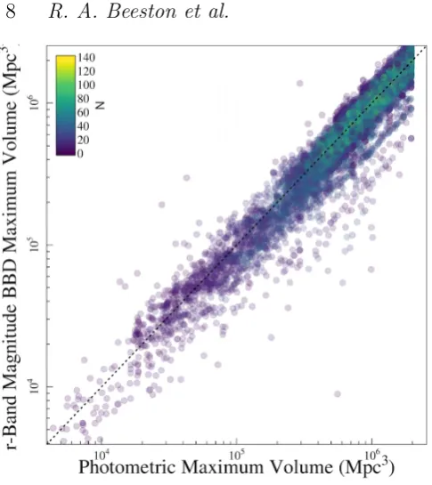
A direct comparison of the maximum volumes derived from both the pVmax and BBD methods is shown in Fig.4 with the points coloured by the average number of galaxies in the BBD bin containing that galaxy across all the MC simulations. The largest deviation from the 1:1 line is seen for galaxies that lie in bins with a small number of galax-ies contributing to the median volume. These volumes are generally low, meaning they are also strongly affected by cos-mic variance. ThepVmaxvalues are systematically higher by 0.8% on average than those derived from the BBD method, which translates to an average offset of 1% in the binned DMF values when determined by the median weighted by the error on the measurement.
Since we compare to the galaxy stellar mass function from W17, who use stellar mass and surface brightness as the BBD axes, it may be argued we should use the same approach. We consider this in Appendix B, and conclude that the Schechter parameters are consistent with ther-band and surface brightness BBDs within uncertainties. We opt to use ther-band magnitude for our second axis here as it
is more in line with the opticalpVmax, and does not depend on stellar properties directly.
Density fluctuations in the GAMA equatorial fields e.g.
Driver et al.(2011);Dunne et al.(2011) have a pronounced effect on the DMF, and so we apply density corrections as calculated by W17 to account for the over- or under-densities present in each of the equatorial fields (see e.g. Loveday et al. 2015). These multiplicative corrections were derived as a function of redshift by determining the local density of the survey at the redshift of the galaxy in question. This is achieved by simply finding the running density as a func-tion of redshift, and convolving this funcfunc-tion with a kernel of width 60 Mpc. These were compared to the fiducial den-sity, taken from a portion of the GAMA equatorial fields with stellar masses above1010Mand0.07<z<0.19. This subset was chosen because of its high completeness level, uni-form density distribution, and low uncertainty due to cosmic variance. To correct the effective volume for galaxyn,Veff,n, we simply multiply by a factor ofδn/hδfito obtainVmax0 .
Figure 4. The maximum effective volumes for our galaxies at
z < 0.1 derived using the pVmax method (x-axis), and BBD method using r-band magnitude and surface brightness as the two selection features (y-axis). The colour of the points is de-termined by the number of galaxies in the BBD bin that each galaxy resides in (Fig3), as shown by the colour bar in the top left corner. We note that the number of galaxies per bin is the median resulting from 1000 Monte Carlo simulations, where we perturb ther-band magnitude and surface brightness within their associated uncertainties.
volume density and therefore tend to add less noise to their given bin than faint galaxies. Once removed, the weights of the remaining galaxies are scaled by the fraction of removed galaxies11.
4.2 The Shape of the DMF
The DMF, derived for the largest sample of galaxies to date, based on the optically selected GAMA sample, is shown in Fig.5using the two methods described in Section4.1to cal-culate volume densities. We have extended the function well below the low dust mass limit of all previous studies; indeed we extend to dust masses∼104Mwhilst dust masses above
104.5M are well constrained. We have therefore extended the observed range of the DMF by∼2 dex inMd compared to e.g.Dunne et al.(2011) and significantly reduced the statis-tical uncertainty compared to previous measurements (with ∼70×the sample size, see Section4.3for more details). The offset at the low-mass end of the DMF seen between the two methods can be attributed to the differences shown in Fig.
4, the sources with the lowest dust mass tend to be those which are nearby and faint, and so most likely to be affected by small number statistics when calculating the BBDVmax values.
11 This has the effect of smoothing the low-mass end of the DMF.
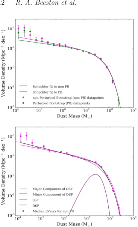
Figure 5.The pVmax(purple) and BBD (blue) dust mass func-tions for the GAMA/H-ATLAS sources at z < 0.1. The data points show the observed values corrected for over and under densities in the GAMA fields (see W17). The solid lines are the best fitting (minimum χ2) single Schechter functions from our SB measurements. Error bars are derived from our PB measure-ments. The total number of sources in each bin is shown in the top panel.
We estimate uncertainties on the volume densities cal-culated here using three techniques. First, using a jackknife method in two different ways: (i) taking random subsamples of the data, and (ii) by splitting the sample by on-sky lo-cation. Second, we perform 1000 bootstrap resamplings on our volume densities to determine the sample errors. We re-fer to this as the simple bootstrap or SB method. Third, we use the bootstrap technique but for each realisation, we also perturb each dust mass by a Gaussian random devi-ate withσset according to the 16-84 percentile uncertainty frommagphys(hereafter the PB method). Unsurprisingly, Poisson noise estimates agree with all these techniques at the high mass end (Md >107.5M), but underestimate the uncertainty in the low dust mass bins (Md <106M). The random jackknife and SB error estimates agree very well (within 0.5 %), whereas the on-sky jackknife uncertainty is around 5 % higher. This is not unexpected since this method will include a component of uncertainty from cosmic vari-ance within the survey volume. By disentangling the statis-tical uncertainty from the cosmic variance uncertainty, the larger uncertainty in the on-sky jackknife suggests an error due to cosmic variance of at least 7 per cent assuming that the difference is due only to cosmic variance. The cosmic variance estimator fromDriver & Robotham(2010)12 sug-gests an error of 16.5 per cent for the full survey volume. This is significantly higher than the effective cosmic vari-ance that we measure, because we make corrections for the
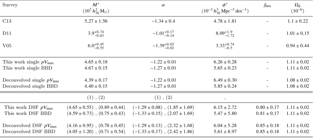
[image:8.595.310.532.106.335.2]Survey M∗ α φ∗ f
mix Ωd
(107h2
70M) (10
−3h3 70Mpc
−3dex−1) (10−6)
C13 5.27±1.56 −1.34±0.4 4.78±1.81 - 1.1±0.22
D11 3.9+−00..7463 −1.01−+00..1714 8.09−+11..972 - 1.01±0.15
V05 6.0+0.45
−0.55 −1.39+0 .03
−0.02 3.33+0 .74
−0.5 - 0.94±0.44 This work singlepVmax 4.65±0.18 −1.22±0.01 6.26±0.28 - 1.11±0.02 This work single BBD 4.67±0.15 −1.27±0.01 5.65±0.23 - 1.11±0.02
Deconvolved singlepVmax 4.39±0.17 −1.22±0.01 6.49±0.30 - 1.08±0.02 Deconvolved single BBD 4.40±0.15 −1.27±0.01 5.85±0.24 - 1.08±0.02
(1) , (2) (1) , (2) ,
This work DSFpVmax (4.65±0.55) , (0.89±0.44) (−1.29±0.08) , (1.85±1.69) 6.15±2.72 0.80±0.17 1.11±0.02 This work DSF BBD (4.59±0.73) , (0.75±0.43) (−1.33±0.15) , (2.07±1.69) 5.47±5.80 0.81±0.17 1.11±0.02
[image:9.595.44.561.106.333.2]Deconvolved DSFpVmax (4.16±0.95) , (0.78±0.45) (−1.29±0.13) , (2.32±1.68) 6.04±5.28 0.85±0.18 1.11±0.02 Deconvolved DSF BBD (4.05±1.20) , (0.71±0.54) (−1.33±0.17) , (2.42±1.86) 5.61±8.97 0.85±0.18 1.11±0.02
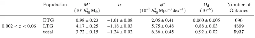
Table 1.Schechter function values for dust mass functions in the literature and this work for both the SSF and DSF fits). The other literature studies include: C13 -Clemens et al. 2013, D11 -Dunne et al. 2011, V05 -Vlahakis et al. 2005. All have been scaled to the same dust mass absorption coefficient used here. TheDunne et al.(2011) DMF includes a correction of 1.42 for the density of the GAMA09 field (Driver et al. 2011) and the fits in this work include the density-weighted corrections from W17. For comparison we include the deconvolved Schechter function fit parameters in the final section of the table (see Section4.4), which are very similar to the ordinary Schechter function parameters. We also include the double Schechter function (DSF), and deconvolved DSF with their major component and minor component listed under (1) and (2) respectively for each non-coupled SF parameter (see Equation3).
density variations within the survey volume. For the rest of this work, we use the simple bootstrap method without perturbation of the dust mass (SB) for the data points. For the uncertaintoes we use the bootstrap with additional per-turbation using themagphysdust mass uncertainties (PB) since this takes into account both the variation within the sample and the uncertainty in the dust mass estimations themselves. As discussed in section 4.4the PB is likely to give biased estimates of the best fit parameters, but since it includes our mass uncertainties, it provides a better estimate of the uncertainties on the best fit parameters.
FollowingDunne et al.(2011), we fit a single Schechter function (SSF) (Schechter 1976) to the observed DMF, using χ2 minimisation to derive the best-fit values forα, M∗ and φ∗ which are the power law index of the low-mass slope, the characteristic mass (location of the function’s ‘knee’), and the number volume density at the characteristic mass respectively. This takes the form (inlogM space):
S(M;α,M∗, φ∗)=φ∗e−10logM−logM
∗
×10logM−logM∗α+1dlogM, (2)
where we have explicitly included the factorln10in the def-inition ofφ∗, such thatφ∗is in units ofMpc−3dex−1.
We fit a Schechter function to each of our bootstrap realisations, and use the median of the resulting values as the best fit value for each parameter. We use the standard deviation between the values to estimate uncertainty on the parameters. The parameters for both the pVmax and BBD fits are quoted in Table 1. Note that cosmic variance will
introduce further uncertainty in our measurements. This will mostly be seen as an increased uncertainty on φ∗, though bothM∗ andαwill also have slightly larger errors.
4.3 Comparing the Dust Mass Function with previous work
We compare the SSF parameters derived here with single Schechter function fits in the literature (Fig.6left and Ta-ble1). We also compare the confidence intervals for our de-rived parameters in Fig.7with previous work. For the first time we are able to directly measure the functional form at masses below5×105Mand determine the low mass slope of the DMF,α. We see that there is a good overall match at the high mass end with theDunne et al.(2011) DMF, but at the faint end, the DMF is steeper than predicted from the
Dunne et al. (2011) function suggesting larger numbers of cold or faint galaxies than expected. We note that theDunne et al. (2011) sample is different to our DMF in two ways (i) it is a dust-selected (or rather 250-µm-selected) sample rather than optically selected and (ii) was drawn from the
H-ATLAS science demonstration phase data, which is only 16 sq deg of the GAMA09 field at z <0.1and is known to be under-dense compared to the other GAMA fields (Driver et al. 2011). Our DMF is also similar to the optically-selected
Vlahakis et al.(2005)13 SSF at the highest masses, though we find a higher space density of galaxies around the ‘knee’
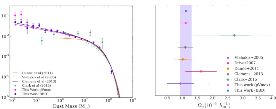
Figure 6. Comparison of the (left) DMF and (right) dust mass densitiesΩdfrom this work with those from the literature. We compare with (i) the blind, localz<0.01galaxy sample fromClark et al.(2015) (ii) the all-sky local star-forming galaxies from the brightPlanck catalogue fromClemens et al.(2013) (iii) the ground-based submm measurements of local optical galaxies fromVlahakis et al.(2005) and (iv) the 222 galaxies out toz<0.1from theH-ATLAS survey (Dunne et al. 2011). Schechter fit parameters are listed in Table1. The dust density parameter (Ωd) measurements are scaled to the same cosmology, with diamonds representing dust-selected measurements and circles representing optically-selected samples. Our work are shown aspVmaxand BBD for the single Schechter fit - SSF to each. The solid error bars onΩdindicate the published uncertainty derived from the error in the fit whilst the transparent error bars indicate the total uncertainty derived by combining the published uncertainty and the cosmic variance uncertainty estimate for that sample (where known). We note that the solid error bars indicating the uncertainty from our bootstrap analysis lie within the point itself for both our BBD andpVmaxvalues. TheDunne et al.(2011) DMF includes the correction factor of 1.42 for the density of the GAMA09 field (Driver et al. 2011) whilst our data points have been weighted by density correction factors from W17. The shaded region emphasises the range ofΩdderived from our observed SSF fits to the DMFs with width showing the error from cosmic variance.
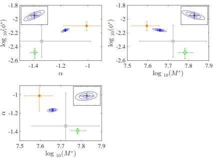
of the function potentially due to the higher redshift limit probed in this study and improvement in statistics in this work. In general, the 2-d parameter comparisons in Fig. 7
show that the DMF in this work has intermediate values of α,M∗andφ∗in comparison to theClemens et al.(2013)14,
Vlahakis et al.(2005), and Dunne et al.(2011) parameters but here we have tighter constraints due to the larger sample of sources. Differences could also arise because of the vari-ation of best-fit parameters with the minimum mass limit of the fit since all the surveys have different mass ranges. We discuss the implications of changing the minimum mass limit of our fits in AppendixC.
The integrated dust mass density parameter Ωd at
z≤0.1is derived by using the incomplete gamma function to integrate down toMd=104M(our lower limit on measure-ment of the form of the DMF). This gives(1.11±0.02) ×10−6
for both the pVmax and BBD methods. For comparison, our Ωd values calculated without imposing this limit are (1.11±0.02) ×10−6 and (1.06±0.01) ×10−6 for the pVmax and BBD methods respectively, so the difference is very small. Previous measurements of Ωd are shown in Fig. 6
(right) (all scaled to same cosmology and κ), we also
re-14 The fit parameters quoted in this work for Clemens et al. (2013) are different to those that appear in their paper and in Clark et al. (2015). The reason for this is that Clemens et al. (2013) did not include theln10factor when calculating their in-tegrated dust densities, and inClark et al.(2015) we erroneously attributed this error to a missing per dex factor in φ∗. In fact their error was only in converting fromφ∗ toρd.
calculate the literature values using the SSF fit parameters from Table1, this ensures that they are integrated down to our mass limit. Our measurement is consistent withDunne et al.(2011),Vlahakis et al. (2005), Clemens et al.(2013) and with the lower range ofDriver et al.(2007) but smaller than theClark et al.(2015) values. However, the latter mea-surement is subject to a large uncertainty due to cosmic variance (46.6 per cent,Driver et al. 2007) in comparison to the 7-17 per cent for this work15. Further discussion on the evolution of the dust properties over cosmic time is provided inDriver et al.(2017).
4.4 Eddington Bias in the Dust Mass Function
Here we check whether our DMF is biased due to the dust mass errors frommagphys. Since the scatter due to the mass error could move galaxies into neighbouring bins in either di-rection, and as the volume density is not uniform, this could have the effect of introducing an Eddington bias (Eddington 1913) into the DMF.Loveday et al.(1992) showed that this bias effectively convolves the underlying DMF with a Gaus-sian with width equal to the size of the scatter in the vari-able of interest (here dust mass) to give the observed DMF. This is valid assuming that the parameter uncertainties, and hence resulting errors, have a Gaussian distribution. Here we test whether we can correct for the Eddington bias in the DMF by deconvolving our observed DMF and attempt to
-1.4
-1.2
-1
-2.6
-2.4
-2.2
-2
-1.8
7.5
7.6
7.7
7.8
7.9
-2.6
-2.4
-2.2
-2
-1.8
7.5
7.6
7.7
7.8
7.9
-1.4
[image:11.595.71.506.118.435.2]-1.2
-1
Figure 7. The confidence intervals for thepVmaxsingle Schechter dust mass function fit parameters derived in this work (blue ellipses) showing the correlation between the fit parameters (insets) and comparison with previous values (note thatφ∗is in units ofMpc−3dex−1). Error bars on our fit parameters are taken from the ∆χ2 =1for each parameter (these are consistent with errors derived from the bootstrap process described in Section4). The contours are from the 1, 2, 3σvalues of∆χ2for the parameter slice centred on the best fit for the non-plotted 3rd parameter. Green denotesVlahakis et al.(2005), orange representsDunne et al.(2011), and grey showsClemens et al.(2013). We note that the error bars on theVlahakis et al.(2005) values were derived using Poisson statistics, and so may be an underestimate of the error in the measurements.
extract the underlying ‘true’ DMF. We expect that any bias in the overall cosmic dust density will be small since galaxies with at least one measurement over 3σ in one of theHerschelSPIRE bands contribute around four times as much to the dust density of the Universe than those without a 3σmeasurement in the FIR regime.
We fit a SSF convolved with a Gaussian, where we es-timate the width of the Gaussian using two methods. First, we derive the width of the convolved function by calculat-ing the mean dust mass error frommagphysas a function of mass (the varying error method). Second, we take the mean value of the error in dust mass around the knee of the single Schechter function where the convolution will have the strongest effect (where the mean error is 0.11 dex, the constant error method). Both produce very similar decon-volved Schechter function fit parameters that are in agree-ment with the traditional Schechter function method within a few per cent. The deconvolved fit parameters derived with constant error are listed in Table 1; this produces a dust mass density of(1.08±0.02) ×10−6 for both thepVmax and BBD DMFs. We find that the traditional single Schechter function is a better fit (∆χ2 ∼0.75) than the deconvolved
constant error function, and the varying error method pro-duces a comparable goodness of fit to the traditional SSF without deconvolution. The reason that the best fit is insen-sitive to the mass errors is that the mass errors are a strong function of mass: for low mass galaxies, the errors are large (∼0.5 dex); while for higher masses (∼ M∗), the errors are small (<0.1 dex). At low masses the DMF is a power law, the slope of which is unchanged when convolved by a Gaussian. At higher masses, near the exponential cut-off, the errors are small, and so the effect on the knee is negligible. We there-fore conclude that there is no strong argument for choosing to use the deconvolved SSF fits instead of the original single Schechter functions, therefore we include the results here for completeness but continue using the original SSF fits throughout the paper.
Figure 8. Top: The pVmax DMF (purple) from the SB mea-surements compared to the DMF derived using the bootstrap perturbed (PB) by the uncertainties in the dust mass estimates frommagphys(the PB DMF, green). The data points show the volume densities in each mass bin and the solid lines are the best fitting (χ2) single Schechter functions, SSF, to the data.Bottom: Comparison of the SSF with the DSF including the major and minor components. The data points show the volume densities in each mass bin, the major and minor components are shown in grey and purple respectively, the overall DSF is shown in ma-genta. Error bars are derived from a bootstrap analysis and the data points have been corrected for over and under densities in the GAMA fields (see W17). The total number of sources in each bin is shown in the top panel.
the perturbed (including the uncertainties in the dust mass from magphys) pVmax DMF (PB DMF). We see that the two DMFs are very similar with fit properties differing by only a few per cent. The largest differences in the DMF are seen at the noisier low dust mass end suggesting the biases are indeed small, we believe this is because the uncertainties in the DMF around the knee are small.
We also perform another test to quantify the bias in-troduced to the DMF by the inclusion of sources with poor FIR constraints. We use the distribution of temperatures of sources with high total FIR signal to noise to define a new temperature prior. Then for each bootstrap sample we draw new temperatures from this prior and adjust the dust
masses accordingly. In this way we perform another kind of perturbed boostrap in which each realisation has a tem-perature distribution that matches the high signal to noise galaxies. We find that the bias introduced to the DMF in this way is very small, and so we believe our DMF is robust. This is discussed in more detail in AppendixA.
4.5 A Double Schechter Fit to the DMF
The issues revealed in Section4.3(and in AppendixC) show-ing the dependence of the SSF fit parameters with the chosen lower mass limit of the SSF fit suggests that the observed DMF is not adequately represented by the SSF. W17 also found that a SSF fit was not sufficient to fit their stellar mass function of the same sample, instead they required a double Schechter function (DSF) fit with the same M∗, but differ-ent faint-end slopes. We therefore follow W17 and fit a DSF
D(M)but unlike W17, we do not couple the twoM∗values, since there is no reason to believe that multiple populations in the dust mass functions would have the same character-istic mass. The DSF is therefore just defined as the sum of two single functions) of the form:
D(M;M1∗,M2∗, α1, α2, φ∗,fmix)=S(M;M1∗, α1, φ∗) ×fmix
+S(M;M2∗, α2, φ∗) × (1−fmix) (3)
where fmixis the fractional contribution of one of the com-ponents. Fig.8compares the DSF with the SSF. The major component of the DSF is similar to the SSF, but the for-mer provides a better fit to the ‘shoulder’ in the data at
M ∼ 107M and results in a reduced χ2 ∼3×lower than the SSF fit. Although the DSF significantly reduces the χ2 of the best fit, the variation of mass errors as a function of mass could introduce this kind of shape in the DMF. We therefore cannot be sure that the DSF represents a funda-mentally better model of the data, and prefer to use the SSF as our standard fit. The best-fit parameters for the DSF are listed in Table1. The dust density for the pVmax DSF fit is1.11±0.02×10⁻⁶, corresponding to an overall fraction of baryons (by mass) stored in dust fmb =(2.51±0.04) ×10
−5,
assuming the PlanckΩb =45.51×10⁻³h−270 (Planck Collab-oration XIII 2016). The DSF therefore returns exactly the same value for dust density as using the simpler SSF. We also note that the improvement in χ2 from SSF to DSF becomes insignificant when the uncertainty due to cosmic variance is included in the fitting process.
It is tempting to link the two Schechter components to early and late-type galaxies, but the parameters of the minor component of the DSF do not match those of the early-types (see Section6). This suggests that the two components of the DSF do not represent physically distinct populations, and so does not provide a better representation of the data.
5 THEORETICAL PREDICTIONS FROM
GALAXY FORMATION MODELS
Next we compare the SSF fit to the DMF from Section4.4
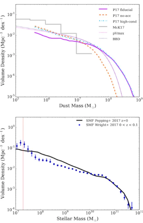
(SAMs) of galaxy formation based on cosmological merger trees fromSomerville et al.(2015) andPopping et al.(2014) and include prescriptions for metal and dust formation based on chemical evolution models. They predict DMFs at dif-ferent redshifts using dust models with dust sources from stars in stellar winds and supernovae (SNe), grain growth in the interstellar medium, and dust destruction by SN shocks and hot halo gas (see alsoDwek 1998;Morgan & Edmunds 2003; Micha lowski et al. 2010; Dunne et al. 2011; Asano et al. 2013;Rowlands et al. 2014;Feldmann 2015; De Vis et al. 2017b). Note that for consistency, we have scaled the Popping DMFs down by a factor of 2.39 in dust mass since their z=0models were calibrated on dust masses for local galaxy samples from theHerschel Reference Survey (Boselli et al. 2010;Smith et al. 2012b;Ciesla et al. 2012) and KING-FISH (Skibba et al. 2011) whereDraine(2003) dust absorp-tion coefficients are assumed. After this scaling, their DMF (based on their SAMs) is consistent with a Schechter func-tion with M∗∼107.9M. In Fig.9(top) we compare three of their z = 0DMF models as defined in Table 2: the so-called fiducial, high-cond and no-acc models. Their fiducial model assumes 20 per cent of metals from stellar winds of low-intermediate mass stars (LIMS) and SNe are condensed into dust grains, with interstellar grain growth also allowed. The high-cond assumes that almost all metals available to form dust that are ejected by stars and SNe are condensed into dust grains, with additional interstellar grain growth. The no-acc model assumes 100 per cent of all metals avail-able to form dust that are ejected by stars and SNe are con-densed into dust grains, with no grain growth in the ISM.
The fiducial and high-cond models overpredict the num-ber density of galaxies in the high dust mass regime, >
107.5M. The no-acc model is the closest model to the ob-served high mass regime of the DMF, though underestimates the volume density aroundM∗compared to our DMF (dot-ted lines in Fig. 9). Both the no-acc and high-cond models are better matches at low masses (<107M), while the fidu-cial model underpredicts the volume density in this regime. This likely suggests that LIMS and SNe have to be more efficient than the fiducial model at producing dust in low dust-mass systems i.e. the dust condensation efficiencies in both stellar sources need to be larger than 0.3, or that the dust destruction and dust grain growth timescales in the fiducial model need to be increased and decreased respec-tively. At high masses, the fiducial and high-cond models appear to be forming too much dust. This implies that dust production and destruction are not realistically balanced in these models. This is likely due to the model introducing too much interstellar gas and metals, which allow for very high levels of grain growth in the ISM.
We note that the no-acc P17 model (without grain growth in the ISM) is likely not a valid model as it assumes 100 per cent efficiency for the available metals condensing into dust in LIMS and SNe which is unphysically high, see e.g. Morgan & Edmunds (2003); Rowlands et al. (2014). Hereafter we no longer discuss this model even though by eye it appears to be an adequate fit to the observed DMF at masses below107M.
[image:13.595.310.538.103.459.2]To investigate the discrepancy between the observed DMF in this work and the predicted SAM DMF from Pop-ping et al.(2017), we first check that the stellar mass func-tion from the SAMs is consistent with the observed galaxy
Figure 9.Top: A comparison with the predictedz =0 DMFs fromPopping et al. (2017) (P17) and McKinnon et al. (2017) (McK17) with the SSF fits derived from the BBD and pVmax methods, see also Table 2. We include three models from P17: the fiducial, no-acc and high-cond models which consist of vary-ing dust condensation efficiencies in stellar winds, supernovae and grain growth in the interstellar medium respectively. The McK17 histogram is their L25n512 simulation atz=0(their Fig. 2). Bot-tom:Comparing thez=0stellar mass functions for the GAMA sources (W17, in blue) with that derived using the SAMs of Pop-ping et al.(2017) (in black). W17 is the SMF of the same optical sample from which our DMF is derived. The vertical line shows the boundary at which W17 fit their data with a Schechter func-tion.
stellar mass function (GSMF) for the GAMA sample in W17 (Fig. 9 bottom). The SMFs at the high mass end are in agreement though the model SMF has a slight overdensity of galaxies in the range 108 < Ms(M) < 109.4, where Ms is stellar mass. If this overdensity of sources were responsi-ble for the discrepancy between the predicted and observed DMFs in the highMdregime, those intermediate stellar mass sources would have to have dust-to-stellar mass ratios of ∼0.5which is again unphysical. We can see this is not the case when comparing the dust-to-stellar mass ratios of the
Model Name Efficiency dust LIMS Efficiency dust Type I/II SNe grain growtha dust destructionb
Carbon otherZ Carbon otherZ SNe halo
(not in CO) (Mg,Si,S,Ca,Ti,Fe) (not in CO) (Mg,Si,S,Ca,Ti,Fe) Popping
fiducial 0.2 0.2 0.15 0.15 Y,tacc,0=15Myr Y Y
high-cond 1.0 0.8 1.0 0.8 Y,tacc,0=15Myr Y Y
no-acc 1.0 1.0 1.0 1.0 N Y Y
McKinnon
McK16 1.0 0.8 0.5 0.8 Y, fixedtacc=200Myr Y N
[image:14.595.41.550.106.230.2]McK17 1.0 0.8 0.5 0.8 Y,tacc,0=40Myr Y Y
Table 2. The dust models used in cosmological predictions of the DMF including three models fromPopping et al.(2017) and two models fromMcKinnon et al.(2016,2017). All of the models presume dust formation in LIMS (low-intermediate stars) in their stellar wind AGB phase and in Type Ia and II supernovae.a - the timescale for interstellar grain growth in Milky Way molecular clouds such that the grain growth timescale of the systemtaccis either fixed or derived fromtacc∝tacc,0nmol−1Z
−1whereZis the metallicity andn molis the molecular number density.b- destruction of dust by either SN shocks in the warm diffuse ISM or via thermal sputtering in the hot halo gas. InPopping et al.(2017) 600Mand 980Mof carbon and silicate dust are assumed to be cleared by each SN event respectively. InMcKinnon et al. (2017) dust destruction is derived in each cell of the simulation, with each SN releasing1051ergs; this is consistent with their shocks clearing out 6800Mof gas.
[image:14.595.89.527.345.673.2]In Fig. 10 we plot the dust and stellar masses from the compilation of local galaxy samples collated in De Vis et al.(2017a,b)16 and compare with P17 and our sample of ∼15,000 sources. Here we can clearly see the cause for the discrepancy between the observed DMF from this work and the model:the model overpredicts the amount of dust in high stellar mass sources, well above any dust-to-stellar ratios ob-served locally. Although the observations show a flattening of dust mass at the highest Ms regime (where early type galaxies are dominating), this is not the case in the SAM. In general the SAM prediction assumes a constant dust-to-stars ratio of ∼0.001 across all mass ranges. The observa-tions however suggest that there is a roughly linear relation-ship untilMs>1010M, after which the slope flattens, with
Md/Ms∼0.001.
Fig.10also suggests thatMd/Msincreases to∼0.025in low stellar mass galaxies (in agreement with Santini et al. 2014;Clark et al. 2015;De Vis et al. 2017a). This is further supported by the stacking analysis carried out in Bourne et al. (2012) whose dust-to-stellar mass trends in different bins of optical colour are added to Fig. 10. These were de-rived by stacking on∼80,000 galaxies in theHerschelmaps, revealing that low stellar mass galaxies had higher dust-to-stellar mass ratios, consistent with these sources having the highest specific star formation rates. Our binned data (black points) are in agreement with local galaxy surveys and the
Bourne et al.(2012) trends: we see that the slope of dust-to-stellar mass flattens at high masses, and that there exists a population of dusty low-stellar-mass sources that the SAM does not predict.
Alternative predictions for a local DMF are provided by
McKinnon et al.(2016,2017, hereafter McK16, McK17). In these models, dust is tracked in a hydrodynamical cosmolog-ical simulation with limited volume. The McK16 dust model is similar to the P17 high-cond model (including interstellar grain growth and dust contributed by both low mass stellar winds and SNe) but has no thermal sputtering component. The updated model from McK17 reduces the efficiency of in-terstellar grain growth and includes thermal sputtering (see Table2). The DMF from McK17 (their L25n512 simulation at z =0) is shown in Fig. 9(top). Their values have been scaled to the same cosmology as used here (they use the same κ and Chabrier IMF as this work). We can see that McK17 predicts fewer massively dusty galaxies than P17 and our observed DMFs. Although their DMF fails to pro-duce enough galaxies in the highest mass bins in Fig.9, the simulated DMF becomes more strongly affected by Poisso-nion statistics in this regime due to the small volume of the simulation.
Possible explanations for the difference between the predicted (P17, Mck17) and observed DMFs at large dust masses are (i) the efficiency of thermal sputtering due to hot gas in the halo has been under or overestimated in these highest stellar mass sources; (ii) the fiducial and high-cond dust models of P17 allow too much interstellar grain growth in highest stellar mass galaxies due to the assumed timescales or efficiencies of grain growth being too high; (iii)
16 these have all been scaled to the same value of κand apart from the Dwarf Galaxy Survey, all galaxy parameters have been derived using the same fitting techniques.
the predicted highest stellar mass galaxies have too little (McK17) or too much (P17) gas reservoir potentially due to feedback prescriptions being too strong/not strong enough, respectively. If the gas reservoir is too high, interstellar met-als can continue to accrete onto dust grains and increase the dust mass. Conversely if it is too low, then the contribution to the dust mass via grain growth will be reduced. We will adress each of these possibilities in turn.
(i) We can test if the amount of dust destruction by thermal sputtering in hot (X-ray emitting) gas could explain the differences in the predicted and observed DMF at the high mass end as McK16 and McK17 already compared the results using dust models without and with thermal sputter-ing respectively. They find that includsputter-ing thermal sputtersputter-ing only makes small changes to the shape of DMF since this affects dust in the halo rather the interstellar medium, this is therefore not likely to be responsible for the disreprancy. (ii) Comparing the dust models in P17, McK16 and McK17 allow us to test the effect of changing the grain growth parameters. The timescale for grain growth is short-est in P17 and McK16 and both those models produce too much dust in the high dust mass regime of the DMF. McK17 has a longer grain growth timescale (tacc,0=40 Myr, Table2) than both P17 and McK16 and this change indeed reduces the volume density of the highest dust mass sources. McK17 also compares the DMFs from the same simulation methods with different dust models and they find that a significantly reduced DMF at the high mass end can be attributed to the longer grain growth timescales.
(iii) Earlier we showed that the galaxies that are re-sponsible for the highest dust mass bins in the P17 DMF have too much dust for their stellar mass (Fig.10). To test whether they have too much dust due to the gas reservoir of the SAM massive galaxies being too high (hence leading to more interstellar grain growth) we refer to the predicted and observed gas mass function comparison inPopping et al.
(2014). There they showed that these are not as discrepant as we see here with the modeled and observed dust mass functions and therefore are likely not responsible for the dis-crepancy in the DMF.
We therefore conclude that it is likely that the inter-stellar grain growth in these massive galaxies is simply too efficient/fast in the P17 and McK16 dust models. In this scenario, the few largest stellar mass galaxies are allowed to form too much dust in the interstellar medium at a rate that is not observed in real galaxies. However, the growth timescale may also be too slow in the McK17 model. All of the P17 high-cond, McK16 and McK17 dust models assume very high dust condensation efficiencies in AGB stars and Type Ia and II SNe. We propose therefore that the most re-alistic dust model must lie somewhere in between these and the fiducial P17 model, with stardust condensation efficien-cies larger than 0.3 but lower than 0.8 and a similar dust grain growth timescale as assumed in P17.