Enhancing student visual understanding of the time evolution of quantum systems

Enhancing student visual understanding of the time evolution of quantum systems

Gina Passante1,* and Antje Kohnle2

1

Department of Physics, California State University Fullerton, Fullerton, California 92831, USA

2

School of Physics and Astronomy, University of St Andrews, St Andrews, KY16 9SS, United Kingdom

(Received 4 September 2018; published 13 February 2019)

Time dependence is of fundamental importance for the description of quantum systems, but is particularly difficult for students to master. We describe the development and evaluation of a combined simulation-tutorial to support the development of visual understanding of time dependence in quantum mechanics. The associated interactive simulation shows the time dependence of an energy eigenstate and a superposition state, and how the time dependence of the probability density arises from that of the wave function. In order to assess transitions in student thinking, we developed a framework to characterize student responses in terms of real and complex mathematical reasoning and classical and quantum visual reasoning. The results of pre-, mid-, and post-tests indicate that the simulation-tutorial supports the development of visual understanding of time dependence, and that visual reasoning is correlated with improved student performance on a question relating to the time evolution of the wave function and the probability density. The results also indicate that the analogy of a classical standing wave for the infinite well energy eigenfunctions may be problematic in cueing incorrect ideas of time dependence.

DOI:10.1103/PhysRevPhysEducRes.15.010110

I. INTRODUCTION

As the research on student understanding of quantum mechanics has grown, the time dependence of quantum systems stands out as one of the most difficult topics for students [1–7]. The time evolution is determined by the time-dependent Schrödinger equation and for a one-dimensional spatial wave function can be written as Ψðx; tÞ ¼PnψnðxÞe−iEnt=ℏ, where ψnðxÞ are the spatial parts of the energy eigenfunctions. The fact that the time evolution comes into the wave function as a complex exponential may be one of the reasons why student conceptual understanding of time evolution has proven so difficult.

Although the wave function for a quantum system evolves in the complex plane, the probability density for the same system lives entirely in the real space. This can lead to students ignoring the important role that the imaginary numbers play in quantum mechanics.

This study extends previous work supporting student understanding of the time evolution of quantum systems [8–12]. We developed research-based resources to promote a visual understanding of the time dependence of the wave functionΨðx; tÞand how this leads to the time dependence

of the probability density. By visual understanding and reasoning, we mean the ability to interpret equations graphically or pictorially and to use these depictions to draw conclusions and justify claims. This study consisted of the development of an interactive simulation and a combined simulation-tutorial, and their refinement using interviews and in-class trials at two institutions across two years. This study addresses the following research questions:

RQ1: To what extent does the simulation-tutorial tran-sition student reasoning about time dependence?

RQ2: Is there a correlation between student performance on questions relating to the time evolution of the wave function or probability density and the type of reasoning (mathematical or visual) used?

RQ1 was addressed using pre- and midtests carried out before and a few days after the simulation-tutorial with no further instruction on the topic. We also discuss interview data that underpin RQ1 in terms of giving insight into common incorrect ideas prior to working with the simu-lation-tutorial and changes in student thinking when going through the activity.

For RQ2, one could hypothesize that a visual model may not help due to its inherent complexity and the fact that translations between representations are difficult and not automatic. RQ2 was addressed using a post-test carried out several weeks after the simulation-tutorial, where the solution could be obtained using mathematical and/or visual reasoning. In order to answer the RQs, we devised a new framework to characterize students’ reasoning in terms of real or complex mathematical and classical or

*

[email protected]

quantum visual reasoning that may be useful for other quantum mechanics contexts.

The key findings of this study are that students who used visual reasoning after (but not before) completing the simulation-tutorial were more likely to answer correctly than students who did not. The simulation-tutorial transi-tioned students’responses from classical visual to quantum visual reasoning about time dependence. The results also indicate that the analogy of a standing wave on a stretched string in relation to the infinite square well energy eigen-functions may generate incorrect ideas about time depend-ence in quantum mechanics.

A. Literature review

1. Research into student thinking

Student understanding of the time evolution of quantum systems has been one of the more commonly researched topics in quantum mechanics physics education research. This is in part due to the fact that all quantum systems evolve in time, so that student thinking can be probed at multiple points throughout instruction. For instance, ques-tions about the time evolution of a system can be asked in the context of the infinite square well and in the context of perturbation theory.

There are several surveys on student conceptual under-standing of quantum mechanics that include questions on the time dependence of quantum states, measurements outcomes, and probability densities [2,5,6]. An analysis of the Quantum Mechanics Survey (QMS) finds that many students do not understand the distinction between solutions of the time-independent and time-dependent Schrödinger equations [5]. On the Quantum Mechanics Conceptual Assessment (QMCA) the questions that deal with the wave function and time evolution have the lowest averages[6]. Finally, Cataloglu and Robinett developed the Quantum Mechanics Visualization Instrument (QMVI) assessment that focused on student conceptual and visual understanding. There are three questions that focused on the time-dependent solutions to the Schrödinger equation. All three of these questions had averages much lower than the overall average[2].

In a 2001 study of student understanding of quantum mechanics across six institutions, Singh found that ques-tions related to the time evolution of expectation values and probabilities were among the most difficult[1]. Singh also reported how students are more likely to think that continuous quantities such as position and momentum are deterministic while more “quantum” quantities, such as spin, are probabilistic[3]. In a study surveying incoming graduate students across several institutions, Singh found that“the most common difficulties with quantum dynamics are coupled with an overemphasis on the time-independent Schrödinger equation.” Several groups have noted that students often incorrectly write the equation for the time evolution of a quantum state by ascribing a single phase to

the entire wave function[3,4,7]. There is also a significant percentage of students who say the wave function has no time dependence[4,7]. In Ref.[7], Emighet al.classified student difficulties with time dependence into four catego-ries:“tendency to confuse the time dependence of different quantum mechanical quantities,” “failure to ascribe the correct time-dependent phases to the wave function,”

“tendency to misinterpret the mathematical formalism used for time dependence in quantum mechanics,” and

“tendency to apply ideas about time evolution that lie outside the model for quantum mechanics.”

2. Analysis frameworks

Much of the research literature on student thinking has been performed using a difficulties framework where the researchers analyze student responses for difficulties, which refer to “common incorrect or inappropriate ideas expressed by students, or flawed patterns of reasoning” [13]. These difficulties can then be addressed by targeted curriculum.

Several analysis frameworks have been developed for use in mathematics-heavy physics courses that focus specifically on the use of math in physics problem solving [14–17]. While these frameworks are each unique, they all assume that mathematical calculations (either trivial or more complex) play a role in solving physics equations that can be identified as separate from physics sense making. Each of these frameworks has their strengths, but a limitation of all of them is that they are best suited for more involved, complex problems that generally require both mathematical and physics reasoning. Additionally, some of these frameworks work best when there is a record of how student thinking evolves over time as they work on a task, such as you would have in an audio or video recording.

Our research questions prompted us to ask fundamental physics questions that students can answer using either mathematical or conceptual physics reasoning, but that do not require both. Additionally, we are interested in the responses of a large number of students through written questionnaires. For these reasons, the current mathemati-cally oriented frameworks are not well suited for our purpose. Our analysis framework, which will be outlined in Sec. II D, was informed by both difficulties and the mathematical frameworks referenced above.

3. Curriculum development

and work by Schiber et al. [12] use a physical prop (transparencies and pipe cleaners, respectively) to help students visualize the wave function. However, even in these cases it is very difficult to make a dynamic connection between the evolution of the wave function and the evolution of the probability density.

The activity we developed draws heavily on a tutorial written by the Physics Education Group at the University of Washington (UW) [8]. The UW QM tutorials have been developed using a model similar to that used to develop the

“Tutorials in Introductory Physics” [19]. They span the content of a two-semester quantum mechanics course and are entirely paper based. Each tutorial is approximately five pages and is designed to take a 45-min class period where students work in small groups with a high level of instructor support. The tutorial on “Time Dependence in Quantum Mechanics”was the inspiration and starting point for our activity. The UW version of the tutorial uses a visual aid of transparencies cut out into a three-dimensional axis to help students visualize the motion of the wave function in the complex plane. In our activity development, we took the visual aid to the next level by developing an activity that builds towards that visual model, affirms it with the use of a simulation, and extends it to show the evolution of the probability density. Although the UW tutorial was the starting point for our activity, the changes required in order to focus on the development of a visual model resulted in a final product that is very different from the original.

II. METHODS

A. Research context

This study was performed at two institutions that differ in terms of educational systems and student populations. The University of St Andrews (StA) is a selective, research-intensive institution in the UK, and California State University Fullerton (CSUF) is a Hispanic-serving, teach-ing-focused institution in the USA. The authors were the instructors of the courses where this research was per-formed. At StA, this study was conducted in a junior-level core quantum mechanics course required of physics majors. The course covers standard wave mechanics including the infinite well, the harmonic oscillator, the hydrogen atom, angular momentum, and ladder operators. At CSUF, this study was conducted in a third-year introduction to quantum mechanics course required of physics majors. The course follows a spins-first approach and begins with spin-1=2 particles and Stern-Gerlach experiments as the basis for the postulates of quantum mechanics before moving on to wave functions in approximately the tenth week of a fifteen week course.

B. Activity structure and description

The activity was designed to scaffold students’ develop-ment of a visual model for the time evolution of a wave

function and how that affects the time evolution of the probability density. In order to achieve this, we combined some of the best aspects of tutorials and simulations.

The combined simulation-tutorial activity is structured in such a way that students begin with tutorial-style questions without simulation support where they construct represen-tations they will later see in the simulation. Students are then directed to the simulation and asked to play around with it for several minutes before attempting the remaining questions with simulation support. This activity structure was guided by the literature on encouraging students to engage actively to construct their own understanding (e.g., Ref. [20]), sketching as a learning strategy to promote visual understanding and reasoning[21–23], and support-ing students when learnsupport-ing with multiple external repre-sentations[24,25]. This general structure is the same as for a combined simulation-tutorial on perturbation theory developed in an earlier study by the authors[26].

The simulation-tutorial was designed as an hour-long classroom activity that could be completed as a homework assignment. The activity and simulation were revised using a pilot study. We describe the revised version in what follows.

The first page of the five-page activity has students consider the ground state of the infinite square well and focus on the value of the function at the center of the well. Students are then asked to plot the time evolution of this value on a two-dimensional complex plane and to connect this graphical evolution to the mathematical expression. The final question before students play with the simulation asks them to consider how they might depict the time evolution of the entire wave function, not just of a single point. One possible representation will become apparent once students engage with the simulation.

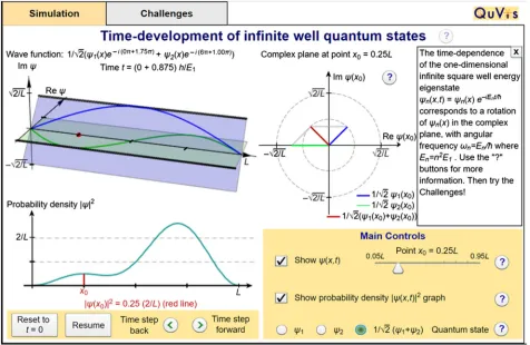
Figure1shows a screenshot of the“Time-development of infinite well quantum states” simulation [27]. The simulation depicts wave functions and probability densities for a one-dimensional infinite square well. The top graphs show two- and three-dimensional depictions of the wave function rotating in the complex plane. The bottom graph shows the corresponding probability density. The math-ematical expression forψðx; tÞ is shown at the top left.

Students can choose the point x₀ along the x axis at which the two-dimensional graph of ψðx₀Þ is displayed; whether to display the ground state, the first excited state, or a superposition of these two states; and which graphs to display. The first excited state energy eigenfunction ψ₂ rotates with an angular frequency four times greater than that ofψ₁, as the energyE₂¼4E₁. For the superposition state (shown in Fig.1), the two-dimensional graph of the complex plane shows howψ at a given point is determined as the vector sum ofψ₁ andψ₂ at that point.

hidden. This is the same graph that students are asked to generate on page one of the activity. Play and step controls at the bottom left can be used to stop and step through the time evolution.

Depicting the time dependence of the wave function as a rotation in the complex plane can address common student difficulties (see Sec.I A 1) that may stem from a lack of a visual model of time evolution: for an energy eigenfunction ψn, it becomes clear in this depiction that the probability density jψ_nj2 remains constant, as the time dependence only changes the phase angle of the wave function curve, not its magnitude. The depiction shows that the energy eigenfunction depends on time, even thoughjψ_nj2does not. The rotation of the energy eigenfunctionψ_nwith constant magnitude shows that it does not decay with time. For the superposition state, the depiction illustrates that the two eigenfunctions cannot be multiplied by a single complex exponential, as the rotation frequency depends on energy. The simulation also shows that the probability density for the superposition stateψ depends on time, as the different rotation frequencies imply that the phase angle betweenψ₁ andψ₂changes with time and thusjψj2changes with time. In the final four pages of the activity, students are asked to relate the graphs they see in the simulation to the ones they sketched on the first page; explain the relation between

different graphs shown in the simulation and link them with the corresponding mathematical expressions; determine the period of each energy eigenfunction both graphically and mathematically; and explore the effect of the relative phase between the energy eigenfunctions in a superposition on the probability density. The activity employs an elicit-confront-resolve strategy [28] using student dialogue questions at several points to directly address difficulties identified in the literature, as well as a model-building approach to help students develop a visual model for the evolution of the wave function and the probability density. For a copy of the combined simulation-tutorial, contact the corresponding author.

C. Study design

The timeline for the study can be seen in Fig. 2. It consists of a pretest that is administered on paper in class after lecture instruction but before the combined simula-tion-tutorial activity, the activity, a midtest administered in FIG. 1. A screenshot of the“Time-development of infinite well quantum states”simulation showing a superposition of the ground and first-excited states.

Pre-test Activity Mid-test 6-8 Post-test weeks

time

class after the activity, and a post-test given weeks later on a class exam. This format was used over the course of two years; the first year as a pilot study in order to revise the simulation and the tutorial questions, the second year as the study that is presented here. The first year pilot study is not discussed further.

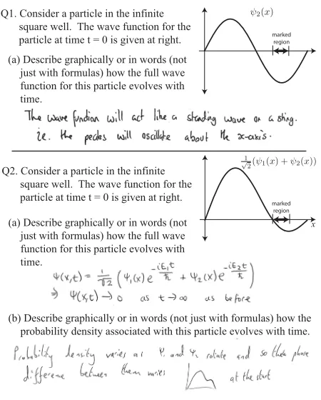
The pre- and midtests were used to address RQ1 to probe transitions in students’reasoning. Abbreviated versions of the pre- and midtest questions and examples of student responses are given in Fig.3. The pre- and midtest questions were adapted from task 1 of a previous study[7], and aimed to assess whether or not students have a correct visual model of the time dependence of the wave function (part a) and the probability density (part b) for an energy eigenstate (ques-tion 1) and a superposi(ques-tion state (ques(ques-tion 2). Identical questions were used in the pre- and midtest. Question 1b (identical in wording to question 2b of Fig. 3) is not discussed further, as answers were almost always correct on the pretest, and students often did not explain their reasoning to this question in the pre- and midtests.

The pretests were completed by students in the class prior to the simulation-tutorial activity. Students were not given feedback on the pretest. The simulation-tutorial

activity was started in class and completed by students as homework. The midtest was run on the day the simulation-tutorial was handed in. All elements excepting the post-test were not assessed and did not contribute to course credit. Students were given approximately 15 min to complete the pre- and midtests: the time was sufficient for essentially all students to complete the tests.

For the analysis of transitions from pre- to midtest used to address RQ1, only students who completed all of the elements shown in Fig.2were included in the study. This led to 66 students being included in this analysis (53 StA and 13 CSUF students), which account for 70% of StA students and 54% of CSUF students enrolled in the courses. Students completed the post-test question shown in Fig. 4 as part of their end-of-course exam. In an effort to answer RQ2, in this paper we analyze student responses to part b (in Sec.III B). This question requires students to determine whether the probability density of the given superposition stateψðx; t¼0Þ ¼ ð1=pffiffiffi2Þ½ψ₁ðxÞ þiψ₂ðxÞ depends on time and to explain their reasoning. Note that the quantum system and the wave function are different to those used in the simulation-tutorial and the pre- and midtests. It is possible to reason mathematically by writing down the expression forψðx; tÞand using this expression to determinejψj2, and/or reason visually by considering the rotation of the ψ₁ and ψ₂ curves in the complex plane. Thus, this question allowed us to address RQ2 by compar-ing the correctness of students’answers and reasoning for visual and mathematical responses.

For the post-test analysis, all students who took part in the simulation-tutorial activity were included in the analy-sis, including students who were not present for the pre- or midtest. This led to 86 students (64 StA and 22 CSUF students) being included for the post-test analysis.

The study design also included individual student inter-views to underpin RQ1 that were conducted prior to the in-class implementation. The aims of the interviews were to

FIG. 3. Abbreviated versions of the three pre- and midtest questions administered before and after the activity discussed in Sec.III A. All three questions also included the instruction:“If it does not depend on time, state so explicitly.”Examples of three different student responses are also shown. Using the framework in Sec. II D, these responses were coded as incorrect classical visual (1a), incorrect complex mathematics (2a), and correct quantum visual (2b).

The spatially symmetric normalized ground state wave function and the antisymmetric normalized first excited state wave function at time t = 0 for a system are shown at right. Assume that the energy E₂ of the first excited state is four times the energy of the ground state E₁.

The system is initially (at time t = 0) in a state given by:

(a) Sketch the probability density for this state at time t = 0. Show your reasoning.

(b) Does the probability density for this state depend on time? Explain your reasoning.

ψ1(x)

ψ2(x)

ψ1(x, t= 0)

ψ2(x, t= 0)

ψ(x, t= 0) =√1

2(ψ1(x) +iψ2(x))

gain qualitative insight into students’ transitions of visual reasoning, to identify particular difficulties in achieving correct visual understanding, and to iteratively revise the simulation and activity. We carried out 13 interviews in total. In eight of the 13 interviews, students worked through the activity using a think-aloud protocol and interacted with the simulation after answering the initial questions without simulation support. Five of the interviews were conducted with students who had completed the simulation-tutorial in class approximately ten months previously, and had a different format: students answered the pre- and post-test questions without simulation support before being asked to use the simulation and revise their answers where needed. Thus, these five students did not work on the simulation-tutorial during the interview.

D. Coding framework

The literature on student difficulties with time depend-ence (Sec. I A 1) and our experience as instructors sug-gested that many of these difficulties could be grouped at a more coarsely grained level as students either disregarding the imaginary component of the wave function or inap-propriately applying a classical picture to the evolution of the wave function. Both of these groupings have a mathematical and a visual aspect to them. For example, Crouse[29]found that students believe the wave function will decay as time progresses. This may be due to treating the time-dependent complex phasee−iEnt=ℏ _{as a decaying} exponential, which would be the case if there was noiin the expression, or it may be a graphical image of a decaying exponential curve that is most salient for students. It has also been seen that students will disregard the imaginary component of the wave function by indicating that as time evolves, the wave function will act as a standing wave where a point of maximum amplitude will decrease to zero, become negative, and then go through zero again as it returns to its largest value [7]. From conversations with students, the description of a one-dimensional standing wave does not necessarily stem from the mathematical expression, but with classical experiences of, for example, a standing wave on a fixed string.

We have developed an analysis framework for student reasoning that makes use of these themes of real versus complex and classical versus quantum. This framework has two main dimensions: mathematical and visual. Each dimension is divided into two bins that can roughly be categorized as classical and quantum. Along the math-ematical dimension this takes the form of using real or complex numbers. Along the visual dimension the responses are divided intoclassicalorquantum. In addition to coding for the type of reasoning on each dimension, we also coded for correctness of reasoning.

This approach allows us to characterize key elements of student difficulties at a more coarsely grained level than individual difficulties, and to group previously identified

difficulties based on common underlying themes. The framework is well suited to answering research questions RQ1 and RQ2 given its focus on the type of reasoning used and the correctness of the reasoning. The framework can be applied to short written responses and does not require interview or video data for implementation.

Along the mathematics dimension, each student was coded as either complex mathematics, real mathematics, or not coded. Complex mathematics was coded if the students wrote an expression for the time evolution and used complex numbers. For example, for question 1a in Fig. 3, a complex mathematics answer might be

“ψ2ðx; tÞ ¼e−iE2t=ℏψ2ðxÞ,” which is a correct expression.

An example of a response coded as incorrect complex mathematics is shown in Fig.3in response to question 2a. Real mathematics was coded if a student provided a mathematical expression such ase−tthat was entirely real if there should have been an imaginary component. If a student provided a written description of an equation, that was also coded as mathematical. Responses that did not include an equation or the description of an equation were

“not coded” along this dimension.

The visual dimension is divided into quantum visual, classical visual, and not coded. If a response involved graphs or a written visual description of the time evolution it was coded as visual. In addition to the examples of an incorrect classical and a correct quantum visual response given in Fig.3to questions 1a and 2b, respectively, TableI gives further examples of visual responses for question 1a. Quantum visual descriptions must be close to a correct description about the wave function rotating in the three-dimensional complex plane. Describing the real and imagi-nary parts separately such as“both the real and imaginary parts of the wave function change as the function oscillates with time” would also be coded as a quantum visual response. Examples of classical visual descriptions (see TableI) include describing the wave function as a classical traveling or standing wave, a purely real wave (or wave packet) sloshing back and forth, or an exponential decay described in words or with a sketch.

It was possible for responses to be coded in both mathematics and visual dimensions, although this was not very common. Additionally, responses that did not provide reasoning (“changes with time but I don’t really know why”), that stated the wave function does not depend on time (“As ψ₂ is an energy eigenstate it [the wave function] does not change with time”) or just stated that the wave function oscillates without further explanation (“over time the [wave] function will oscillate”) were not coded in either category, as these responses did not have enough detail to be considered visual or mathematical in nature.

correctness. Classical visual reasoning and real mathemati-cal reasoning were always incorrect. The large majority of the quantum visual responses were considered correct; however for responses that were given the complex mathematics code, it was possible for that reasoning to be correct or incorrect.

The pre- and midtest data were coded independently by two student researchers, one at CSUF and one at StA. The pilot study data were used for training, with discussion of disagreements following the initial coding. For the study presented here, the interrater agreement for math-based reasoning and correctness of math-based reasoning was high throughout for the three questions, with agreement >90% for reasoning and >86% for correctness. The interrater agreement for visual reasoning and correctness of visual reasoning was somewhat lower, with agreement

>70%throughout for the three questions for reasoning and correctness of reasoning. After coding by the student researchers, all coding disagreements were discussed by the authors and resolved. This resulted in the final codes used for the analysis shown in Sec.III A.

The authors coded post-test question b shown in Fig.4 according to the same coding scheme as the pre- and midtests. The percent agreement of the two coders ranged from 88% for correctness of visual reasoning to 99% for the answer, with an average agreement of 95%. After dis-cussion, all of the coding discrepancies were resolved.

III. RESULTS

Section III A addresses RQ1: to what extent does the simulation-tutorial transition student reasoning about time dependence? This section discusses transitions from the pretest to the midtest for the time evolution of an energy eigenstate, a superposition state and the probability density for a superposition state. Using the post-test results, Sec. III B addresses RQ2: Is there a correlation between student performance on questions relating to the time evolu-tion of the wave funcevolu-tion or probability density and the type of reasoning (mathematical or visual) used? SectionIII C under-pins RQ1 by giving insight from the interviews how the simulation-tutorial changes student thinking and the persistent difficulty of a classical standing wave.

A. Transitions from pre- to midtest 1. Evolution of an energy eigenstate

Question 1a on the pre- and midtest asked students to describe the time evolution of an energy eigenstate (see Fig.3). As described in Sec.II D, student responses were coded for the type of reasoning used (classical or quantum visual, and real or imaginary mathematical) and the correctness of their reasoning.

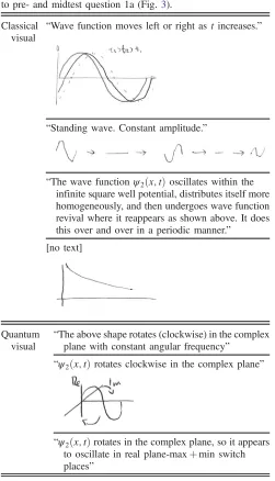
TABLE I. Examples of student responses coded as either classical visual or quantum visual. All examples are responses to pre- and midtest question 1a (Fig.3).

Classical visual

“Wave function moves left or right astincreases.”

“Standing wave. Constant amplitude.”

“The wave functionψ₂ðx; tÞoscillates within the infinite square well potential, distributes itself more homogeneously, and then undergoes wave function revival where it reappears as shown above. It does this over and over in a periodic manner.”

[no text]

Quantum visual

“The above shape rotates (clockwise) in the complex plane with constant angular frequency”

“ψ2ðx; tÞ rotates clockwise in the complex plane”

“ψ2ðx; tÞrotates in the complex plane, so it appears

to oscillate in real plane-maxþmin switch places”

TABLE II. The percentage of pre- and midtest responses to question 1a that were coded as visual, and the percentage of correct reasoning of these responses (e.g., 11.8% of the St Andrews visual responses to pretest question 1a were correct). The responses are shown for StA (N¼53) and CSUF (N¼13) students separately. Also included are the percentage of answers that were not coded. Responses that included both mathematical and visual reasoning are included as visual reasoning in the table. Errors are the standard errors of a proportion.

1a pre 1a mid

StA Visual reasoning 64.26.6 81.15.4 % correct 11.84.4 88.44.4 Not coded 22.65.7 15.14.9

CSUF Visual reasoning 46.213.8 84.610.0

% correct 0 63.613.3

Table II shows the fraction of responses using visual reasoning and the fraction of these responses that used correct reasoning (e.g., 11.8% of the St Andrews visual responses to pretest question 1a were correct). The results for the two institutions are separated to illustrate that the increase in percent of students using visual reasoning and the percentage of those with correct reasoning is present at both institutions. The small fraction of responses with mathematical reasoning are not shown in this and the following tables (TablesII–IV); hence the percentages for the reasoning types do not add to 100%. Because of the very different educational environments (including pre-requisite courses and order of quantum mechanics instruc-tion) it is not instructive to compare the performance at each institution.

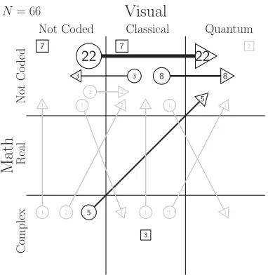
TableIIshows that the percentage of students coded as using visual reasoning as well as the percentage of those students using correct reasoning increases at both StA and CSUF after the activity. The transitions between pre- and midtest responses are illustrated in more detail in the consistency plot in Fig. 5. The consistency plots have the math dimension on the vertical axis and the visual dimension on the horizontal axis. Arrows show a transition from pretest coding (circles) to midtest coding (triangles) and the number indicates how many students made that particular transition. Arrows and boxes with less than three students have been colored gray in the figures to allow for better visualization of overall trends. Squares indicate students who were coded in the same category for the pre- and midtest. The top left-hand category is for responses that were not coded to use either math or visual reasoning in their answers. These responses were either blank or did not include enough explanation to code along

either dimension. More information on the coding scheme can be found in Sec. II D. The consistency plots in Figs. 5–7 combine the data from both institutions, as these plots show transitions at the individual student level and we are interested in global trends (which are similar across both institutions).

For question 1a we see that on the pretest, most responses were either not coded (18=66), coded as classical visual (36=66), or coded as complex mathematical (18=66). On the midtest after completing the activity, 81% of the responses are coded in the visual dimension (54=66) with 45 of these (representing 83% of the visual responses) in the quantum visual category. Only nine students (of the initial 36) continued to describe the time evolution in a classical visual way. Remember that it is not necessary for students to use both mathematical and visual reasoning, as a complete answer can consist of one or the other.

Using the language of Wittmann and Black[30], we see that the quantum visual category is an attractor, that is, many more responses end there rather than start there. Additionally, we see that there is avoid(empty categories) in the real math row, which tells us that students very rarely use real math to describe the time evolution. We do not see any true starbursts where many responses originate but they all move to different directions. The movement in our diagrams is very clearly towards the quantum visual region.

2. Evolution of a superposition state

Question 2a on the pre- and midtest asked students to describe the time evolution of a superposition of energy eigenstates (see Fig. 3). Table III shows the fraction of responses using visual reasoning and the correctness of this reasoning.

The consistency plot for question 2a (see Fig.6) shows similar trends to question 1a in that the quantum visual category is an attractor. On this question we see some circulationpairs where there are some regions that give and take in relatively the same amounts (see the pair of three and two student lines between the not coded and classical visual as an example). However, we do not see this in large numbers. Here we find 39=66 responses in the quantum visual category on the midtest and 16 students describing

FIG. 5. Response transitions from pre- and midtest question 1a. Circles are pretest codes and triangles are the midtest codes for mathematical and visual. Note that the data presented are for the type of reasoning used, not correctness. Response patterns with less than three students are in gray to help illustrate overall trends.

TABLE III. The percentage of pre- and midtest responses to question 2a that were coded as visual, and the percentage of correct reasoning of these responses.

2a pre 2a mid

StA Visual reasoning 45.36.8 86.84.7 % correct 4.22.7 60.96.7 Not coded 43.46.8 13.24.7

CSUF Visual reasoning 15.410.0 69.212.8

% correct 0 44.413.8

the evolution in a classical visual way. There are a small number of transitions along the mathematical (vertical) axis, however, the bulk of the transitions occur along the visual (horizontal) dimension.

3. Probability density for a superposition state

Question 2b asks about the evolution of the probability density of the superposition state (see Fig.3). Because the state is a superposition of two (nondegenerate) energy eigenstates, each component eigenstate rotates in the complex plane at a different angular frequency. This results in a time dependence of the probability density when the (modulus of the) wave function is squared.

Table IV shows the fraction of responses using visual reasoning and the correctness of this reasoning. Note that for this question, approximately three-quarters of the responses were not able to be coded along either dimension on the pretest, and this went down to approximately 40% on the midtest. The consistency plot in Fig. 7 shows the transitions in more detail. The quantum visual category is still a large attractor with 32 responses on the midtest, up from 5 on the pretest.

4. Discussion of all three questions

In response to RQ1, on all three questions both the fraction of responses using visual reasoning and the correctness of reasoning increased from the pre- to the midtest. The low pretest results indicate that very few students had correct visual understanding prior to the activity. Of the 396 responses in total across the pre-and midtests (six questions each with 66 responses), 30 responses were coded as both mathematical and visual (and these were included in the visual count in TablesII–IV).

On all questions we found that the percentage of responses that were not coded decreased, indicating that students were better able to justify their answers after completing the activity. The percentage of responses using only mathematical reasoning was low throughout (≤12% for each question), presumably as the wording of the pre-and midtest questions cued visual reasoning. For all three questions combined, the percentage of correct reasoning for responses coded as only mathematical was 73.9% on the pretest (23 responses) and 71.4% on the midtest (7 responses).

Comparing the results from Secs. III A 1 and III A 2 shows that the time development of the wave function for the superposition state (question 2a) is more difficult for students than the energy eigenstate (question 1a). This is not surprising given that the superposition state is more complicated in terms of the visual features. About a quarter of the visual answers coded as incorrect for midtest question 2a had productive elements in terms of describing the two eigenfunctions moving in and out of phase or rotating in the complex plane, but then also included incorrect ideas such as the wave function sloshing back and forth in the real plane (which is a correct description of the probability densityjψðxÞj2) or the given functionψðxÞ rotating in the complex plane. Examples are student responses“The peaks of the wave function will oscillate FIG. 6. Response transitions from pre- and midtest question 2a. FIG. 7. Response transitions from pre- and midtest question 2b.

TABLE IV. The percentage of pre- and midtest responses to question 2b that were coded as visual, and the percentage of correct reasoning of these responses.

2b pre 2b mid

StA Visual reasoning 17.05.2 54.76.8 % correct 44.46.8 82.85.2 Not coded 73.66.1 39.66.7

CSUF Visual reasoning 7.77.4 46.213.8

% correct 0 83.310.3

from left to right as the individual wave functions rotate in the Re-Im [real-imaginary] plane”and“max [maximum] and min [minimum] will rotate around the x-axis.”Some answers coded as incorrect for question 2a only had an incomplete description and did not specify the rotation in the complex plane, such as “it rotates around the imaginary axis.”

B. Post-test results

This section considers part b of the end-of-course post-test shown in Fig.4. In contrast to the pre- and midtests, the question text did not cue a particular type of reasoning. This question expects students to explain how the time depend-ence of the probability density comes about and thus focuses on student understanding of both the time evolution of a superposition state and the corresponding probability density.

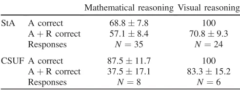
As described in Sec.II C, all students who took part in the simulation-tutorial activity were included in the analy-sis (N ¼86), including students who were not present for the pre- or midtest. Table V shows the percentage of students in the post-test with the correct answer and with the correct answer and reasoning for both institutions, separated into the type of reasoning used.

Eight responses used both mathematical and visual reasoning and are included in TableVas visual reasoning. Six of these eight responses used predominantly visual reasoning, with the mathematical reasoning only consisting of the different complex exponentials in the formula for the wave function ψðx; tÞ. Thirteen students used neither mathematical nor visual reasoning and are not included in the table; of these thirteen students, only five (38.5%) had the correct answer, and none had correct reasoning.

In response to RQ2, TableVindicates that students using visual reasoning were more correct in their responses than students using only mathematical reasoning. We carried out multidimensional chi-square tests to assess differences in the

correctness of the responses depending on the type of reasoning. Students using neither mathematical nor visual reasoning were not included in these tests. Given that there were no significant differences between the two institutions the data from both institutions were combined for these tests. Because of cell frequencies having less than five counts, an exact significance test was selected for Pearson’s chi-square for the correctness of the answer. There was a significant relationship between type of reasoning and correctness of answer: χ2ð2; N¼73Þ ¼10.019, exact p¼0.002, two tailed. The relationship between type of reasoning and correctness of both answer and reasoning was not signifi-cant:χ2ð2; N¼73Þ ¼2.943,p¼0.086, two tailed.

Students using mathematical reasoning to determine the probability density jψðx; tÞj2 sometimes applied incorrect manipulation of formulas, for example, neglecting the cross terms when squaring the expression for

ψðx; tÞ ¼ 1ffiffiffi

2

p ½ψ1ðxÞe−iE1t=ℏþiψ2ðxÞe−iE2t=ℏ;

claiming that these cross terms give zero due to orthogon-ality, or including only one of the two cross terms. Incorrect visual answers included only describing the motion of the probability density without explaining how it arises, assuming wave packet dispersion or assuming that only the real component of the wave function determines the probability density. However, the majority of students using visual reasoning gave detailed and correct answers such as “Yes, the probability densityjψj2depends on time because it is a superposition state of ψ₁ and ψ₂. These energy eigenstates rotate [in] the complex plane with different angular velocities. This means that at different times ψ₁ andψ₂will be added up differently forjψj2 because they are at different positions in the complex plane.”It is worth noting that all of the responses with correct visual reason-ing gave a detailed account of how the time dependence of the probability density arises from the time dependence of the wave function.

The post-test results are encouraging in that a third of the students used visual reasoning to explain their answer when they were not cued to do so and under exam conditions. All of these students arrived at the correct answer, although some had incorrect reasoning. Of the students with correct visual reasoning, most made a very clear connection between the evolution of the wave function and the evolution of the probability density. This indicates that visual ing can be advantageous over purely mathematical reason-ing, that can lead to incorrect algorithmic manipulation without sense making of the physical situation.

C. Student interviews

As described in Sec. II C, individual student interviews were conducted to gain qualitative insight into students’ transitions of visual reasoning and to identify particular TABLE V. The percentage of post-test responses to part b with

the correct answer (“A”, top row) and both correct answer and reasoning (“AþR”, middle row), separated into students who used mathematical reasoning or visual reasoning. Responses that included both mathematical and visual reasoning are included as visual reasoning in the table. The bottom row shows the number of responses used to determine each of the percentages. The responses are shown for StA (N¼64) and CSUF (N¼22) students separately. Errors are the standard errors of a proportion.

Mathematical reasoning Visual reasoning

StA A correct 68.87.8 100

AþR correct 57.18.4 70.89.3

Responses N¼35 N¼24

CSUF A correct 87.511.7 100

AþR correct 37.517.1 83.315.2

difficulties in achieving correct visual understanding in order to underpin RQ1. The interviews indicated that developing a correct visual model of time dependence is challenging and requires careful scaffolding of the simu-lation-tutorial due to a persistent incorrect model of the time dependence being a classical standing wave.

In six of the thirteen interviews, students initially stated that the time dependence of an energy eigenfunction looked graphically just like a classical standing wave, i.e., a string clamped at two ends oscillating at the first harmonic, second harmonic, etc. Five of these students made sketches depicting the standing wave at different times, including times where the amplitude of the wave function is zero everywhere, i.e., the graph is a horizontal line. Thus, these students did not consider the complex nature of the wave function or the normalization of the probability density.

In what follows, we illustrate this difficulty with excerpts from one of these interviews. Question 1 of the activity asks students to sketch the ground state energy eigenfunction ψ1ðxÞ. The student sketches the correct shape and states

“…it would be a single bump. And then atL=2because that’s one [the amplitude is maximal, here assumed to be one], that’s the fundamental frequency. I kind of look at a string that’s clamped at both ends. That’s the first harmonic.”

The student thus states that the shape of the ground state eigenfunction consists of a single peak with maximal amplitude at L=2, and relates this shape to the first harmonic of a classical standing wave.

Question 4a of the activity asks students to plot the time evolution ofψ₁ðx¼L=2; tÞon a given graph of a complex plane by plotting the values ofe−iE1t=ℏ_{at special times. The} student is able to determine the time evolution as a circle in the complex plane.

Question 4b asks for a sketch of the ground state at the time whereE₁t=ℏ¼3π=2. The student’s response to this question is inconsistent with question 4a and reverts back to a classical standing wave: the student initially makes four sketches of a standing wave, showing a positive peak, a horizontal line, a negative peak and a horizontal line again, and explains their sketches by stating “So there I’m thinking of a string again.”Asking the student to elaborate on why they hold this idea, they respond

“…because of the eigenvalues for the energy: they kind of represent harmonics numbers and as they go up you get more. You fit more half wavelengths into your wave function if it’s bound for example in the infinite square well … because that corresponds so heavily with the harmonics. … The shape, because it changes as the energy, as the eigenvalues go up and it seems to change in basically exactly the same way as the harmonics change. The only difference is that you get the temporal solution tied onto the end of it.”

Thus, the fact that the shapes of the infinite square well energy eigenfunctions are identical to the harmonics of a classical standing wave seems to indicate to the student that the time dependence will also be the same as for a classical standing wave.

Later in the activity, this same student comes to realize that the time dependence is a rotation rather than a classical standing wave, and is able to recognize how their original idea of a classical standing wave would violate the normalization of the wave function:

“So it is rotating in the complex plane as opposed to bouncing up and down like a string so it’s going round. …So it has moved from þ1[the student assumes the amplitude is one] to the imaginary plane and it’s going to move down to -1 and then move up to minus i and then just keep on rotating. So it doesn’t flatten out at any point, because if it did flatten out the probability of finding it anywhere in that place would have been zero because you would square it, magnitude squared and that would give you nothing so your particle would have to disappear and appear like over and over, which would make absolutely no sense.”

The student recognizes that if the wave function “ flat-tened out”to just a horizontal line, then the corresponding probability density would be zero everywhere and thus there would be no quantum particle in the infinite well.

These excerpts are illustrative of the transition from classical to quantum visual understanding of time evolution as seen in the consistency plots. They show this transition over the course of the activity from one of the interviews. More generally, we found an initial disconnect in the interviews between the mathematical representation of time evolution (which none of the students had difficulty with) and the visual representation. None of the students with an incorrect classical visual model initially noticed the incon-sistency between their correct mathematical expression and their incorrect classical visual representation. We also found that the classical standing wave model was persistent (and sometimes coexisted with the quantum visual model) unless explicitly addressed via an activity question that asks students to agree or disagree with this model using the visualizations in the simulation.

IV. DISCUSSION AND IMPLICATIONS FOR INSTRUCTION

A. Discussion of findings

which differ in terms of educational systems, curriculum, and student populations.

The consistency plots in Sec. III A show a striking difference in frequencies of responses coded as real math (which can be interpreted in our context as“classical”math) and as classical visual. While classical visual responses such as describing a classical traveling or standing wave, a real wave packet sloshing back and forth, or a decaying wave function are common in the pretest (making up 45.5% of all responses and 90.9% of visual responses for questions 1a and 2a combined), only two responses used real math in these same pretest questions. This may indicate that most students know the correct mathematical form of the time dependence, but that this knowledge is only algorithmic without an underlying conceptual understanding.

Transitions between pre- and midtests were assessed by developing a framework that characterizes student reason-ing in terms of real or complex mathematical and classical or quantum visual responses. This framework captures student difficulties with time evolution seen in previous studies. The framework may be useful to characterize student responses for a range of quantum mechanics contexts. For example, in the context of Stern-Gerlach experiments[31], student responses sketching or describ-ing a continuous sweep of deflections or incorrect zero deflection on the output screen would be classical visual responses, and probability calculations using the square of an inner product rather than the modulus square would be real mathematical responses. In the context of measurement [32], responses that the energy distribution remains unchanged after measurement due to energy conservation or that diffusion leads to an equally weighted superposition over all states with time would be classical visual responses, and responses that indicate only the real part of the coefficients in an energy superposition state deter-mine the probability of an energy measurement outcome would be real mathematical responses. However, the framework is limited in that it may not be useful for topics where working with fully real quantities is sufficient (e.g., when only the spatial part of the energy eigenfunction is needed such as finding perturbed eigenfunctions using time-independent perturbation theory), or for topics focus-ing on the formalism of quantum mechanics.

While the current simulation-tutorial activity transitions students towards quantum visual reasoning, this work has a number of limitations. The simulation-tutorial only has a limited focus on translating between different representa-tions and developing representational fluency (the ability to construct and interpret representations and translate between them accurately and quickly [33]). In the post-test only 8 of 86 students (9.3%) used both mathematical and visual reasoning in their responses. Considering the midtest, most students used only mathematical or only visual reasoning to answer all questions on a given test. The fraction of students using only mathematical or only visual

reasoning to answer all three questions (1a, 2a and 2b) was 84.9% for StA and 76.9% for CSUF, respectively. The results cited here only pertain to the students included in the study. Studies with students from further institutions would be needed to generalize the outcomes.

There was a shift in some of the incorrect ideas seen on the midtest away from the classical visual. Most of the common incorrect ideas from the pretest showed up in very small numbers on the midtest. For example, only 3.0% of students incorrectly stated that the time dependence is the same as a classical standing wave, 6.1% of students stated the wave function dies away with time, and 6.1% of students stated that the wave function has no time dependence (for both institutions combined). However, there was the appearance of a new quantum visual incorrect idea in response to question 2a on the midtest where students stated that the entire curve of the initial wave function would rotate around thex axis in the complex plane. This response was only given by 7.6% of students, but it was not a response we had seen previously nor that we had found in the literature. Intriguingly, it is the visual equivalent of the common mathematical difficulty seen in multiple studies[3,4,7]of ascribing a single phase to the entire wave function. Future versions of the activity will take this idea into account.

B. Implications for instruction: Standing wave analogy

This study has implications for quantum mechanics instruction. The results indicate that using the analogy of a standing wave on a string in relation to the infinite square well energy eigenfunctions may promote incorrect classical ideas about the time dependence of the energy eigenfunc-tions. This analogy is used in an introductory quantum phenomena course at the University of St Andrews (roughly equivalent to an algebra-based introductory phys-ics course in the USA), that was taken as a first course in quantum physics by the majority of St Andrews students in this study. The course uses the analogy of a standing wave on a stretched string in terms of the relation between the de Broglie wavelength and the length of the well:L¼nλ=2, as well asψ being zero outside of the well. This analogy is not used at CSUF and there were very few cases of students describing the energy eigenfunction as a standing wave.

mapped. In terms of the classical standing wave analogy, it may be that the time dependence becomes part of the mapping given the widely used images and animations of standing wave patterns that are well known to students.

An alternative explanation could be that students rec-ognize that both the real and imaginary components of the wave function form standing waves that are out of phase, or that students recognize that there exists the imaginary component but then assume that the imaginary part of the wave function is irrelevant. However, the interviews and written responses in this study indicate that this explanation is unlikely, as the majority of responses describing standing waves did not make any reference to the imaginary part of the wave function in their visual reasoning.

The standing wave analogy may also promote an incorrect objectlike or trajectorylike interpretation of the wave function (termed by Elby as“ What-you-see-is-what-you-get”[36]), given that it describes the physical location of the stretched string. While not seen in our study, the standing wave analogy may also promote incorrect ideas of the amplitude of the wave function being related to the energy of a quantum particle, as energy is related to amplitude for a classical standing wave but not for a quantum-mechanical wave function [37,38].

In summary, the findings of this study indicate that the analogy of a standing wave on a stretched string is best avoided or used with care in a way that makes its limitations clear to promote a correct understanding of quantum-mechanical time dependence.

C. Conclusions and future work

In summary, the combined simulation-tutorial helped students develop a correct visual understanding of the time

evolution of the wave function and how this leads to the time evolution of the probability density. The post-test results indicate that visual reasoning is correlated with improved student performance on questions relating to time development.

Future versions of the activity will take the remaining incorrect ideas seen with low frequencies in the mid- and post-tests into account, including quantum visual incorrect ideas that had not previously been reported in the literature, such as the superposition state curve rotating in the complex plane without changing its shape.

In addition, a greater focus on representational fluency in the simulation-tutorial activity may help to further reduce incorrect ideas and promote expertlike reasoning and will be a focus of future development. The coding framework developed here is useful for such future work, given that it captures inconsistencies between mathematical and visual reasoning for responses coded as both.

ACKNOWLEDGMENTS

The authors would like to thank Sam Lloyd for the coding of the simulation, and all students who participated in the evaluation studies and provided feedback on the materials. We would like to acknowledge the work of Michael Williams on the initial analysis of the pilot study data and carrying out individual interviews. We thank Ridwan Pfluger and Zong Yu Wang for coding the full dataset to test for reliability and Benjamin Schermerhorn for helpful comments on the draft manuscript. We thank Trevor Smith for his code and assistance in generating our consistency plots. We thank the University of St Andrews for funding the development of simulations.

[1] Chandralekha Singh, Student understanding of quantum mechanics,Am. J. Phys.69, 885 (2001).

[2] E. Cataloglu and R. W. Robinett, Testing the development of student conceptual and visualization understanding in quantum mechanics through the undergraduate career,Am. J. Phys.70, 238 (2002).

[3] C. Singh, Transfer of learning in quantum mechanics,AIP Conf. Proc.790, 23 (2005).

[4] C. Singh, Student understanding of quantum mechanics at the beginning of graduate instruction,Am. J. Phys.76, 277 (2008).

[5] G. Zhu and C. Singh, Surveying students’understanding of quantum mechanics in one spatial dimension,Am. J. Phys. 80, 252 (2012).

[6] H. R. Sadaghiani and S. J. Pollock, Quantum mechanics concept assessment: Development and validation study,

Phys. Rev. ST Phys. Educ. Res.11, 010110 (2015).

[7] P. J. Emigh, G. Passante, and P. S. Shaffer, Student under-standing of time dependence in quantum mechanics,Phys. Rev. ST Phys. Educ. Res.11, 020112 (2015).

[8] University of Washington Physics Education Group, Tu-torials in Physics: Quantum Mechanics.

[9] Physics Department Oregon State University, Paradigms Quantum Activities, http://physics.oregonstate.edu/ portfolioswiki/topic:quantum.

[10] C. Singh, Interactive learning tutorials on quantum me-chanics,Am. J. Phys.76, 400 (2008).

[11] University of Colorado PhET, PhET Quantum Bound States simulation,https://phet.colorado.edu/en/simulation/ legacy/bound-states.

[13] P. R. L. Heron, Empirical investigations of learning and teaching, Part I: Examining and interpreting student thinking, inInternational School of Physics Enrico Fermi Course CLVI, edited by E. F. Redish and M. Vicentini (2004), pp. 341–350.

[14] E. Kuo, M. M. Hull, A. Gupta, and A. Elby, How students blend conceptual and formal mathematical reasoning in solving physics problems,Sci. Educ.97, 32 (2013). [15] T. J. Bing and E. F. Redish, Epistemic complexity and the

journeyman-expert transition,Phys. Rev. ST Phys. Educ. Res.8, 010105 (2012).

[16] B. Modir, J. D. Thompson, and E. C. Sayre, Students’ epistemological framing in quantum mechanics problem solving,Phys. Rev. Phys. Educ. Res.13, 020108 (2017). [17] B. R. Wilcox, M. D. Caballero, D. A. Rehn, and S. J. Pollock, Analytic framework for students’use of math-ematics in upper-division physics, Phys. Rev. ST Phys. Educ. Res.9, 020119 (2013).

[18] S. B. McKagan, K. K. Perkins, M. Dubson, C. Malley, S. Reid, R. LeMaster, and C. E. Wieman, Developing and researching PhET simulations for teaching quantum me-chanics,Am. J. Phys. 76, 406 (2008).

[19] L. C. McDermott and P. S. Shaffer,Tutorials in Introduc-tory Physics, Prentice Hall Series in Educational Innova-tion (Prentice Hall, Englewood Cliffs, NJ, 2002). [20] M. T. H. Chi, Active-Constructive-Interactive: A

Concep-tual Framework for Differentiating Learning Activities,

Top. Cognit. Sci.1, 73 (2009).

[21] S. Ainsworth, V. Prain, and R. Tytler, Drawing to learn in science,Science333, 1096 (2011).

[22] R. Tytler, V. Prain, P. Hubber, and B. Waldrip, Construct-ing Representations to Learn in Science(Springer Science & Business Media, New York, 2013).

[23] M. Stieff, Improving representational competence using molecular simulations embedded in inquiry activities, J. Res. Sci. Teach.48, 1137 (2011).

[24] S. Ainsworth, DeFT: A conceptual framework for consid-ering learning with multiple representations,Learn. Instr. 16, 183 (2006).

[25] M. A. Rau, Conditions for the Effectiveness of Multiple Visual Representations in Enhancing STEM Learning,

Educ. Psychol. Rev.29, 717 (2017).

[26] A. Kohnle and G. Passante, Characterizing representational learning: A combined simulation and tutorial on perturba-tion theory, Phys. Rev. Phys. Educ. Res. 13, 020131 (2017).

[27] University of St Andrews QuVis Quantum Mechanics Visualization Project, QuVis time development simulation,

www.st-andrews.ac.uk/physics/quvis/simulations_html5/ sims/TimeDevelopment/TimeDevelopment.html. [28] L. C. McDermott and P. S. Shaffer, Research as a guide for

curriculum development: An example from introductory electricity. Part I: Investigation of student understanding,

Am. J. Phys.60, 994 (1992).

[29] A. Crouse, Research on Student Understanding of Quan-tum Mechanics as a Guide for Improving Instruction, Ph.D. thesis, University of Washington, 2007.

[30] M. C. Wittmann and K. E. Black, Visualizing changes in pretest and post-test student responses with consis-tency plots,Phys. Rev. ST Phys. Educ. Res. 10, 010114 (2014).

[31] G. Zhu and C. Singh, Improving students’understanding of quantum mechanics via the Stern-Gerlach experiment,

Am. J. Phys.79, 499 (2011).

[32] G. Passante, P. J. Emigh, and P. S. Shaffer, Examining student ideas about energy measurements on quantum states across undergraduate and graduate levels, Phys. Rev. ST Phys. Educ. Res.11, 020110 (2015).

[33] M. De Cock, Representation use and strategy choice in physics problem solving,Phys. Rev. ST Phys. Educ. Res. 8, 020117 (2012).

[34] D. Gentner, Structure Mapping: A Theoretical Framework for Analogy,Cogn. Sci.7, 155 (1983).

[35] A. B. Markman and D. Gentner, Structure mapping in the comparison process,Am. J. Psychol.113, 501 (2000). [36] A. Elby, What students’learning of representations tells

us about constructivism, J. Math. Behav. 19, 481 (2000).

[37] M. C. Wittmann, J. T. Morgan, and L. Bao, Addressing student models of energy loss in quantum tunnelling,Eur. J. Phys.26, 939 (2005).