Equilibrium and stability properties of collisionless current sheet models

(1)

EQUILIBRIUM AND STABILITY PROPERTIES OF

COLLISIONLESS CURRENT SHEET MODELS

Fiona Wilson

A Thesis Submitted for the Degree of PhD

at the

University of St Andrews

2013

Full metadata for this item is available in

Research@StAndrews:FullText

at:

http://research-repository.st-andrews.ac.uk/

Please use this identifier to cite or link to this item:

http://hdl.handle.net/10023/3548

This item is protected by original copyright

(2)

Equilibrium and Stability Properties of

Collisionless Current Sheet Models

Fiona Wilson

Thesis submitted for the degree of Doctor of Philosophy

of the University of St Andrews

(3)

(4)

Abstract

The work in this thesis focuses primarily on equilibrium and stability properties of collisionless

current sheet models, in particular of the force-free Harris sheet model.

A detailed investigation is carried out into the properties of the distribution function found by

Harrison and Neukirch(2009b) for the force-free Harris sheet, which is so far the only known nonlinear force-free Vlasov-Maxwell equilibrium. Exact conditions on the parameters of the

dis-tribution function are found, which show when it can be single or multi-peaked in two of the velocity space directions. This is important because it may have implications for the stability of

the equilibrium.

One major aim of this thesis is to find new force-free equilibrium distribution functions. By using

a new method which is different from that ofHarrison and Neukirch (2009b), it is possible to find a complete family of distribution functions for the force-free Harris sheet, which includes the

Harrison and Neukirch(2009b) distribution function. Each member of this family has a different dependence on the particle energy, although the dependence on the canonical momenta remains

the same. Three detailed analytical examples are presented. Other possibilities for finding further collisionless force-free equilibrium distribution functions have been explored, but were

unsuc-cessful.

The first linear stability analysis of theHarrison and Neukirch (2009b) equilibrium distribution function is then carried out, concentrating on macroscopic instabilities, and considering

two-dimensional perturbations only. The analysis is based on the technique of integration over

un-perturbed orbits. Similarly to the Harris sheet case (Harris,1962), this is only possible by using approximations to the exact orbits, which are unknown. Furthermore, the approximations for the

Harris sheet case cannot be used for the force-free Harris sheet, and so new techniques have to

be developed in order to make analytical progress. Full analytical expressions for the perturbed current density are derived but, for the sake of simplicity, only the long wavelength limit is

(5)

(6)

Declarations

I, Fiona Wilson, hereby certify that this thesis, which is approximately 29000 words in length,

has been written by me, that it is the record of work carried out by me and that it has not been

submitted in any previous application for a higher degree.

I was admitted as a research student in September 2008 and as a candidate for the degree of Doctor

of Philosophy in September 2009; the higher study for which this is a record was carried out in

the University of St Andrews between September 2008 and June 2012.

Date: Signature of Candidate: .

I hereby certify that the candidate has fulfilled the conditions of the Resolution and Regulations

appropriate for the degree of Doctor of Philosophy in the University of St Andrews and that the

candidate is qualified to submit this thesis in application for that degree.

Date: Signature of Supervisor: .

In submitting this thesis to the University of St Andrews we understand that we are giving

per-mission for it to be made available for use in accordance with the regulations of the University

Library for the time being in force, subject to any copyright vested in the work not being affected thereby. We also understand that the title and the abstract will be published, and that a copy of the

work may be made and supplied to any bona fide library or research worker, that my thesis will

be electronically accessible for personal or research use unless exempt by award of an embargo as requested below, and that the library has the right to migrate my thesis into new electronic forms

as required to ensure continued access to the thesis. We have obtained any third-party copyright

permissions that may be required in order to allow such access and migration, or have requested the appropriate embargo below.

The following is an agreed request by candidate and supervisor regarding the electronic

(7)

Embargo on all of electronic copy for the fixed period of two years on the following ground:

 publication would preclude future publication

(8)

Publications

This thesis contains work which has been adapted from the following refereed publications:

1. F. Wilson & T. Neukirch, ’A Family of One-Dimensional Vlasov-Maxwell Equilibria for the Force-free Harris Sheet’, Phys. Plasmas 18, 082108 (2011)

2. T. Neukirch,F. Wilson & M.G. Harrison, ’A Detailed Investigation of the Properties of a Vlasov-Maxwell Equilibrium for the Force-free Harris Sheet’, Phys. Plasmas 16, 122102

(9)

(10)

Acknowledgements

Thanks to:

• Thomas Neukirch, for the guidance and support over the course of my PhD, and for giving

me the opportunity to continue my research in St Andrews.

• Mum, Dad, Louise and Joanna, for the numerous ways in which you’ve helped and

sup-ported me throughout my life so far!

• The Dundee City girls, for all the hilarious moments and great memories over the years.

(11)

(12)

Introduction

1.1 Background

Most of the matter on the Earth occurs in one of three states: solid, liquid, or gas. In the whole of the visible universe, however, it is estimated that over 99% of the matter takes the form of a

’fourth state of matter’, known as plasma. Most plasmas can be described as ionised gases, formed when a neutral gas is heated to a sufficiently high temperature, such that the electrostatic forces

binding electrons to atomic nuclei are overcome (Dendy,1994), meaning that the electrons and positively charged ions can then move freely. Due to the ionisation, the behaviour of a plasma is strongly influenced by electromagnetic fields, and so it will exhibit different and more interesting

behaviour than a neutral gas. As described by, for example,Krall and Trivelpiece(1973), the term ’fourth state of matter’ comes from the fact that heating a solid results in a change of state into a liquid which, when heated further, changes state into a gas, and heating the gas further still results

in an ionised gas, which can be classed as a plasma provided certain conditions are satisfied (e.g.

Chen,1995). This thesis will be concerned only with ionised gases, but it should also be noted that conducting fluids and even solids can be classified as plasmas, provided they contain enough

free charged particles such that their behaviour is dominated by electromagnetic forces (Boyd and Sanderson,1969).

Examples of naturally occurring plasmas visible from the Earth’s surface are lightning and auroras.

Such plasmas are relatively uncommon, however, due to the low temperature and high density of

the Earth’s atmosphere (Krall and Trivelpiece,1973). Consequently, to study plasmas experimen-tally, they must be man-made in the laboratory, and much of laboratory research in plasma physics

is concerned with controlled thermonuclear fusion as a possible source of renewable power for the

future (e.g.Goedbloed and Poedts,2004).

Although the natural occurrence of plasma on Earth is very rare, in the rest of the universe it occurs

almost everywhere. Examples from our solar system include the Sun, solar wind, and planetary magnetospheres and ionospheres. Due to the abundance of plasma in the universe, a good

under-standing of the physics of plasmas is essential for an underunder-standing of many astrophysical activity

processes. It is generally believed that the magnetic field is the source of energy for many of these processes and, therefore, the storage of magnetic energy and its conversion into other forms of

(17)

1.1 Background 2

energy (bulk flow, heat, non-thermal energy) is now one of the core parts of theoretical plasma

astrophysics. Typical examples of activity processes in our solar system are magnetospheric sub-storms, solar flares, and coronal mass ejections.

A key process for magnetic energy release and conversion is magnetic reconnection - a process which changes the connectivity of field lines. This requires the plasma to be non-ideal. However,

the high temperatures and low densities of many astrophysical plasmas imply that they should

be very close to ideal, thus prohibiting the occurrence of magnetic reconnection. This apparent contradiction can be resolved by noticing that a plasma only needs to be non-ideal in a small

region for magnetic reconnection to become possible. Of particular importance are so-called

’current sheets’ - regions of large electric current density that are strongly localised in one spatial direction.

Due to their strong localisation, current sheets are very well described by one-dimensional

equilib-rium models. Using MHD, the task of finding such models is very simple. In many astrophysical plasmas, however, the length scales over which the current density is believed to vary are often

microscopic. In such cases, it is more appropriate to use kinetic plasma equilibria. In tenuous, hot

plasmas, collisions are very rare, and thus Vlasov-Maxwell theory has to be used.

Part of the work in this thesis, therefore, will focus on one-dimensional, non-relativistic,

quasineu-tral Vlasov-Maxwell equilibria, that is equilibria depending on only one spatial coordinate

(cho-sen here to be thez-coordinate). In such a set-up, the spatial invariance in thex- andy-directions means that the canonical momentum is conserved in both directions. The total particle energy

(the Hamiltonian) must also be conserved, due to the time-independence of the problem. Thus, the distribution functions will depend on these three constants of motion. There are many

exam-ples of collisionless equilibria of this type (e.g.Tonks,1959;Weibel,1959;Grad,1961;Morozov and Solov’ev,1961;Hurley,1961;Harris,1962;Bertotti,1963;Hurley,1963;Nicholson,1963;

Sestero,1964,1966;Sestero and Zannetti,1967;Lam,1967;Parker,1967;Lerche,1967;Davies,

1968;Alpers,1969;Su and Sonnerup,1971;Kan,1972;Lemaire and Burlaga,1976;Roth,1976;

Mynick et al.,1979;Lee and Kan,1979a,b;Greene,1993;Roth et al.,1996;Attico and Pegoraro,

1999;Mottez,2003,2004;Fu and Hau,2005;Yoon et al.,2006). There are also a small number of known examples of such equilibria for force-free fields (Sestero,1967;Channell,1976;Bobrova and Syrovatskiˇi,1979;Bobrova et al.,2001;Harrison and Neukirch,2009b), which are fields sat-isfyingj×B = 0, such that the magnetic field and current density are aligned with each other. Such fields can be used to model low-beta plasmas, such as that of the solar corona. Finding

col-lisionless distribution functions for force-free field profiles is, however, a highly non-trivial task, which is reflected in the fact that relatively few examples are known. Of these known examples,

(18)

1.2 Definition of a Plasma 3

Knowledge of collisionless force-free equilibria is important for gaining a deeper

understand-ing of both macroinstabilities, such as the collisionless tearunderstand-ing mode, from which collisionless reconnection can result (e.g. Schindler, 2007), and microinstabilities, which can result from a non-Maxwellian distribution function (e.g.Gary,2005). An important microscopic plasma phe-nomenon is that of wave-particle interactions, such as Landau damping (e.g.Boyd and Sanderson,

2003;Gary,2005), in which an exchange of energy can take place between plasma waves and par-ticles that are moving with the same phase speed. In MHD models, the velocity space distribution of the particles is not taken into account, and so microscopic plasma phenomena cannot be

stud-ied. Although microinstabilities will not be considered in this thesis, it is important to note that

kinetic models allow for investigations of a more diverse range of phenomena than MHD models.

Further discussion of the main points above will be given in the remainder of the present chapter.

The definition of a plasma will be discussed in more detail in Section1.2. The kinetic and MHD

approaches for modelling plasmas will be described in Section1.3. In Section1.4, a discussion of both MHD and Vlasov-Maxwell equilibria will be given. It should be noted that, although the

main focus of the work in this thesis is on Vlasov-Maxwell equilibrium theory, a discussion of

MHD equilibria is given to illustrate the differences from Vlasov-Maxwell equilibria, and also because the MHD context is useful for introducing force-free magnetic fields. In the final section

of the chapter, the main aims of this thesis will be given.

1.2 Definition of a Plasma

As stated in the previous section, most plasmas are ionised gases. It is wrong, however, to assume

that all ionised gases can be described as plasmas, since all gases will be ionised to some degree,

however small. Chen(1995) describes a plasma as ’a quasineutral gas of charged and neutral particles which exhibits collective behaviour’. This definition will be explained further in the

remainder of the present section, and three criteria will be given, which must be satisfied to allow

an ionised gas to be described as a plasma.

The term ’collective behaviour’ refers to the fact that the motion of charged particles induces

electromagnetic fields, which then have an effect on the motion of other charged particles in the

plasma. This occurs over a long range, due to the fact that as the distance between two regions of plasma,r, is increased, the volume of plasma in one region that can affect the other increases as

r3, even though the Coulomb force between the two original regions decreases as1/r2. Therefore, the long-range Coulomb force is important in determining the behaviour of a plasma, which means

that it will exhibit different and more interesting behaviour than a neutral gas.

(19)

1.2 Definition of a Plasma 4

will be true ifλD L, where Lis a typical length scale of the problem, andλD is the Debye length, defined as

λD =

0kBTe

nee2

1/2

, (1.1)

where0 is the permittivity of free space,kB is Boltzmann’s constant,Te is the temperature of the electrons ande is the charge of an ion. The Debye length is the distance over which any charge imbalance is shielded out from the rest of the plasma. IfλD L, therefore, then only a small volume is affected by a charge imbalance, in comparison to the length scaleL, and so the electric fields which arise do not have an overall effect on the behaviour of the plasma. When

any charge imbalance is introduced, the electrons quickly move to establish neutrality, which

causes fluctuations about the equilibrium position (Boyd and Sanderson,2003). These fluctuations oscillate at a frequency known as the electron plasma frequency, given by

ωpe =

nee2

0me

1/2

, (1.2)

whereme = 9.1094×10−31kg is the mass of an electron. An alternative expression for the Debye length in terms of this frequency is

λD =

vth,e

ωpe

, (1.3)

wherevth,e= (kBTe/me)1/2is the electron thermal velocity.

The number of electrons in a Debye sphere (a sphere of radiusλD) is given by

Λ = 4π 3 nλ

3

D, (1.4)

whereΛis known as the plasma parameter. The plasma will exhibit collective behaviour ifΛ1.

A third criterion which a plasma satisfies is that the short-range binary collisions between charged

particles and neutral atoms occur over a much longer time scale than that over which the oscillatory motion due to collective behaviour occurs. This is required to ensure that the majority of particles

do not recombine into atoms, which would cause the ionised gas to behave as a neutral gas.

Denoting the typical binary collision time scale asτb, and the typical time scale of the collective interactions asτc, the condition isτc τb, which can also be written asωcτb 1, whereωcis the typical oscillation frequency (= 1/τc).

(20)

1.3 Plasma Models 5

1. λD L 2. Λ1

3. τcτb.

1.3 Plasma Models

1.3.1 Kinetic (Microscopic) Description of a Plasma

The kinetic description of a plasma is centred around the assumption that, for each particle species s, with massmsand chargeqs, there exists a single particle distribution functionfs(r,v, t), whose evolution is described by the general kinetic equation

∂fs

∂t +v· ∂fs

∂r +

qs

ms

(E+v×B)·∂fs

∂v =

∂fs

∂t

c

, (1.5)

where(∂fs/∂t)cis the rate of change offswith time due to collisions. The expression

f(r,v, t)d3rd3v (1.6)

gives the number of particles of speciessin the six-dimensional phase space volumed3rd3v =

dxdydzdvxdvydvz, centred at(r,v), at timet. Once the distribution function is known, a number of macroscopic quantities can be obtained from it by taking velocity moments, which involves

multiplying by different powers of the velocity and then integrating over velocity space. The

zeroth order velocity moment is obtained by multiplying byv0 and integrating, which defines the density of particle speciessas

ns=

Z ∞

−∞

fsd3v, (1.7)

whered3v = dvxdvydvz, and it is assumed that the distribution function has been normalised appropriately. The first order velocity moment, obtained by multiplying byv and integrating, defines the bulk flow velocity for speciessas

us=

1

ns

Z ∞

−∞

vfsd3v. (1.8)

Another important quantity is the pressure tensor, with the(i, j)component given by

Pij =

X

s

ms

Z ∞

−∞

(21)

1.3 Plasma Models 6

= X

s

ms

Z ∞

−∞

wi,swj,sfsd3v, (1.9)

wherewi,s = vi−ui,sis the deviation from the average velocity,vi (ui,sis the drift velocity of speciessin thei-direction).

The charge and current densities are defined in terms ofnsandusas

σ = X

s

qsns, (1.10)

j = X

s

qsnsus, (1.11)

Knowledge of the distribution function is crucial, therefore, as it allows the charge and current

densities to be calculated, from which the magnetic and electric field profiles can then be found

via Maxwell’s equations of electromagnetism (e.g.Fleisch,2008). These consist of:

• Amp`ere’s law,

∇ ×B=µ0j+µ00

∂E

∂t, (1.12)

which states that an electric current,j, and a time-varying electric field,∂E/∂t, give rise to a circulating magnetic field,B. The second term on the right-hand side of Equation (1.12) is known as the displacement current, and can be neglected if typical speeds are less than

c= 2.99792458×108ms−1, the speed of light in a vacuum. The quantities

µ0 = 4×107Hm−1 and0 = 1/(µ0c2)are the permeability and permittivity of free space,

respectively.

• The solenoidal condition,

∇ ·B= 0, (1.13)

which states that magnetic monopoles cannot exist.

• Faraday’s law,

∇ ×E=−∂B

∂t, (1.14)

which states that a time varying magnetic field,B, induces a circulating electric field,E.

• Gauss’ law,

∇ ·E= σ

0

(22)

1.3 Plasma Models 7

Photosphere Corona Number densityn(m−3) 8×1022 1×1015

TemperatureT (K) 6×103 2×106

Magnetic field strength B (T) 2×10−1 1×10−2

Debye lengthλD (m) 2×10−8 3×10−3 Plasma parameterΛ 2 1×108

Table 1.1: Typical parameter values for the solar corona (corresponding to an active region) and so-lar photosphere (corresponding to a sunspot). The values have been taken fromSchindler(2007).

which states that the electric flux passing through a closed surface is proportional to the

total charge within that surface.

The kinetic equation and Maxwell’s equations form a self consistent system of equations, since

the magnetic and electric fields depend on the distribution function through the charge and current

densities, given by Equations (1.10) and (1.11), and the distribution function in turn depends on the fields through the kinetic equation (1.5).

The collision term on the right hand side of Equation (1.5) is, in general, a ’complicated, non

linear, integral function off’ (Boyd and Sanderson,1969). It is stated bySchindler(2007) that such a term is the result of Coulomb collisions between charged particles, which are ’based on

electric fluctuations in the Debye sphere’, a sphere with radiusλD, whereλDis the Debye length, given by Equation (1.1). It is also stated that the typical Coulomb collision terms scale asln(Λ)/Λ, whereΛis the plasma parameter given by Equation (1.4), which gives the number of electrons in a Debye sphere. Using the definition (1.1) of the Debye length, the plasma parameter can be

written as

Λ = 4π 3

0kB

e2

3/2

Te3/2

n1e/2

, (1.16)

which clearly scales asTe3/2/n1e/2. Coulomb collisions can, therefore, be neglected for values of this ratio which make the plasma parameter very large, such thatln(Λ)/Λis negligible. This is the case for plasmas with a sufficiently high temperature and low density. Such plasmas are

de-scribed as collisionless, because the collision term in Equation (1.5) can be neglected completely. Table1.1shows typical parameter values for the solar corona, and solar photosphere (values from

Schindler,2007). This table shows that the plasma in the solar corona, for example, is approxi-mately collisionless, due to typical temperatures being in the region of2×106K, with the typical number density being in the region of1×1015m−3, which givesΛ = 1×108. The plasma of the solar photosphere, however, is an example of a plasma for which collision terms are

(23)

1.3 Plasma Models 8

giving a value of just 2 for the plasma parameter. It should be noted, however, that the photosphere

contains a large amount of neutrals due to the lower temperature (only a small fraction of the gas is ionised) and, as such, much of the collisions occur between neutrals and protons, as opposed to

collisions between charged particles.

In a collisionless plasma, the mean free path of collisions,λc, is much larger than the length scale,

L, over which the macroscopic fields vary, so that

λcL. (1.17)

An alternative way to view this is that the collision frequency,Ωc, is less than the characteristic frequency,ω, which describes the time rate of change of the macroscopic fields, so that

Ωcω. (1.18)

For a collisionless plasma, the evolution of the distribution function is described by the Vlasov

equation,

∂fs

∂t +v· ∂fs

∂r +

qs

ms

(E+v×B)·∂fs

∂v = 0, (1.19)

and the above equation, together with Maxwell’s equations (1.12)-(1.15), form the Vlasov-Maxwell

system of equations. The left hand side of Equation (1.19) is the total time derivative offs, since

dfs(r,v, t)

dt =

∂fs

∂t + ∂fs

∂r ·

dr

dt + ∂fs

∂v ·

dv

dt, (1.20)

wheredr/dtanddv/dtare given by the equations of motion for a particle of massmsand charge

qsmoving in an electromagnetic field:

dr

dt = v, (1.21)

dv

dt = qs

ms

(E+v×B). (1.22)

Equations (1.21) and (1.22) are the characteristic equations of the Vlasov equation, and thus the characteristic curves are simply the particle trajectories. The Vlasov equation, therefore, states

that the distribution function must be constant along particle trajectories.

1.3.2 Fluid (Macroscopic) Description of a Plasma

(24)

1.3 Plasma Models 9

mechanics together with Maxwell’s equations of electromagnetism. In the fluid approach, all

variables depend only on space and time, since the distribution function is assumed to be close to Maxwellian everywhere. The MHD equations can be derived from the kinetic equations, as

described in a number of textbooks (e.g.Boyd and Sanderson,1969;Bittencourt,1986;Dendy,

1994;Schindler,2007). The derivation will not be given here, however, since the primary focus of the work in this thesis is on Vlasov theory, and MHD will be discussed only briefly in order to

highlight the differences from the Vlasov approach.

The resistive MHD equations are given by

∂ρ

∂t +∇ ·(ρv) = 0, (1.23)

ρ

∂v

∂t +v· ∇v

= j×B− ∇p, (1.24)

∂

∂t+v· ∇ p ργ

= γ−1

ργ ηj

2_, _(1.25)

∇ ×E = −∂B

∂t, (1.26)

∇ ·B = 0, (1.27)

∇ ×B = µ0j, (1.28)

E+v×B = ηj, (1.29)

whereρis the density of the plasma,pthe pressure,γ the polytropic index, andηthe resistivity.

Equation (1.23) is the mass continuity equation, Equation (1.24) is the equation of motion,

Equa-tion (1.25) is the energy equation, and Equations (1.26)-(1.28) are the remaining three Maxwell equations (Gauss’ law is not needed since it is assumed that the plasma is quasineutral). Equation

(1.29) is the resistive form of Ohm’s law, which couples Maxwell’s equations to the fluid

equa-tions through the plasma velocity,v. It describes the motion of the plasma as it moves through a magnetic field,B, and electric field,E.

In ideal MHD (e.g.Schindler,2007;Goedbloed and Poedts,2004;Freidberg,1987), it is assumed that the plasma is a perfect conductor, such that the resistivity,η, can be neglected. Ohm’s law, given by Equation (1.29), then becomes the ideal Ohm’s law

E+v×B= 0, (1.30)

and the energy equation (1.25) becomes

∂

∂t+v· ∇ p ργ

= 0. (1.31)

These equations imply that magnetic field lines move with the plasma. so they are ’frozen’ into

(25)

1.4 Plasma Equilibria 10

the conditions of ideal MHD, which precludes the occurrence of non-ideal activity processes such

as magnetic reconnection. This contradiction can, however, be explained by the fact that current sheets can form, where ideal MHD breaks down, and resistive MHD must then be used to model

the plasma dynamics.

1.4 Plasma Equilibria

1.4.1 MHD Equilibria

In the present section, static equilibria of the MHD equations will be considered, for which∂/∂t= 0andv= 0(e.g.Neukirch,1998;Biskamp,1993;Schindler,2007). MHD equilibria are discussed here in order to a) explain some terminology that will later be used also for Vlasov-Maxwell equilibria, and b) to introduce some one-dimensional MHD equilibria whose Vlasov-Maxwell

counterparts will be discussed later.

Setting∂/∂t = 0 andv = 0in the MHD equations (from Section1.3.2) gives the equations of magnetohydrostatics (MHS) as

j×B = ∇p, (1.32)

∇ ×B = µ0j, (1.33)

∇ ·B = 0. (1.34)

An equation of state or an energy equation is also required to complete the system of equations.

Note also that the electric field can be written asE = ∇φ, whereφis a scalar potential, since Faraday’s law (1.26) gives∇ ×E= 0.

Equation (1.32) is the momentum equation, which now has the form of a force balance equation,

and states that there must be a balance between the Lorentz forcej×Band the pressure gradient ∇p. Equations (1.24) and (1.25) are Amp`ere’s law and the solenoidal condition. Note also that the

continuity equation (1.23) is automatically satisfied, and so, when neglecting gravity, the density

does not appear in the equilibrium equations. It can, therefore, be chosen in line with the physics of the problem.

Using Amp`ere’s law (1.33) to eliminate the current densityjfrom the momentum equation (1.32), as well as using the vector identity

(∇ ×B)×B= (B· ∇)B−1

2∇(|B|

(26)

gives

∇p = 1

µ0

(∇ ×B)×B

= B· ∇B

µ0

− ∇

B2

2µ0

, (1.36)

whereB=|B|. The first term in the second line of Equation (1.36) represents a magnetic tension force, and the second term is a magnetic pressure force.

For cases where the gradient of the plasma pressure,∇p, can be neglected, the momentum (or

force balance) equation (1.32) reduces to

j×B= 0, (1.37)

which implies that the current arising from the magnetic field is parallel to the magnetic field,

µ0j=∇ ×B=α(r)B, (1.38)

wherer = (x, y, z). A magnetic field which satisfies Equations (1.37) and (1.38) is said to be a force-free field. Taking the divergence of Equation (1.38) gives

∇ ·(αB) = ∇ ·(∇ ×B),

⇒α∇ ·B+B.∇α = 0,

⇒B· ∇α = 0, (1.39)

where the solenoidal condition (1.27) has been used, together with the vector identities

∇ ·(∇ ×B) = 0, (1.40)

∇ ·(αB) = α∇ ·B+B· ∇α. (1.41)

Equation (1.39) states that the derivative ofαin the direction ofBvanishes, meaning thatαmust be constant along field lines. Ifαis constant with respect tor, thenBis said to be a linear force-free field. Ifαvaries withr, however, thenBis said to be a nonlinear force-free field. In this case, αremains constant along a given field line, but varies from field line to field line. Note also that,

ifj= 0, thenBis said to be a potential field.

The plasma beta is defined as the ratio of the plasma pressure,p, to the magnetic pressure,B2/2µ0:

β = p

(B2_/₂_µ 0)

(27)

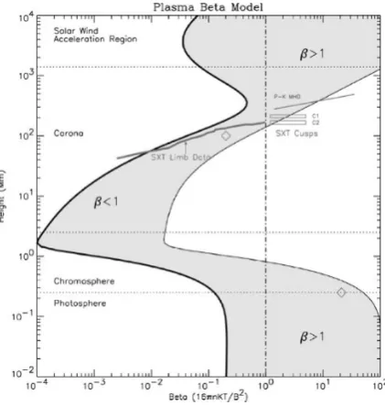
whereB2=B_x2+B_y2+B2_zin Cartesian coordinates. Force-free fields can be used to model low-beta plasmas, since the pressure gradient can be neglected ifβ << 1 (if the magnetic pressure is much greater than the plasma pressure). This situation arises in the solar corona, where the

field can be treated as being approximately force-free. Figure1.1 shows estimates of how the

plasma beta varies for different regions on the Sun, from a model by Gary (2001). It shows that, for the most part, the plasma beta in the solar corona is less than one (this is also true for

the chromosphere), but in the photosphere and solar wind, it is greater than one, meaning that the force-free description would not be appropriate for these plasmas, since the plasma pressure

[image:27.595.192.403.278.500.2]

cannot be neglected.

Figure 1.1: Plot showing how the plasma beta varies for the different regions on the Sun (shaded region). It is less than one throughout most of the solar corona and the chromosphere, and greater than one for the photosphere and solar wind. The boundaries of the shaded region come from two models: one of a plage, the other of the umbra of a sunspot. FromGary(2001).

The simplest solutions of the MHS equations are one-dimensional solutions. In a Cartesian coor-dinate system, assuming that the variation is in thez-direction, this type of solution is known as a

sheet pinch, given by

B = B(z), (1.43)

p = p(z). (1.44)

For a one-dimensional equilibrium depending onz, the magnetic field must be of the form

(28)

sinceBz must vanish in order to satisfy force balance. The field lines will, therefore, be straight lines in planes parallel to thex-y-plane, and hence there will be no magnetic tension force.

The momentum equation (1.36) gives the force balance equation for a one-dimensional

equilib-rium as

d dz

p+ B

2

2µ0

= 0, (1.46)

whereB2 =B_x2+B_y2. This implies that the sum of the plasma and magnetic pressures (the total pressure) is constant,

p+ B

2

2µ0

=ptotal=constant. (1.47)

1.4.1.1 The Harris Sheet

An example of a sheet pinch is the Harris sheet model (Harris,1962). This is a well known model for a one-dimensional current sheet, and has been widely used in studies of plasma instabilities.

Note thatHarris(1962) actually found this as a Vlasov-Maxwell equilibrium. The MHD counter-part will first be introduced here, and the Vlasov-Maxwell case will be discussed later.

The magnetic field of the Harris sheet is given by

BHarris = B0(tanh(z/L),0,0), (1.48)

where B0 is a constant and L is a parameter which specifies the thickness of the sheet. The

pressure is given by

PHarris=

B₀2

2µ0

1

cosh2(z/L) +Pb, (1.49)

wherePbis a constant background pressure. Solving Amp`ere’s law (1.33) gives the current density as

j_Harris = B0

µ0L

0, 1

cosh2(z/L),0

. (1.50)

(1.51)

Figure1.2 (from Harrison, 2009) shows a plot of normalised magnetic field, pressure and cur-rent density profiles for the Harris sheet, and a field-line plot is shown in Figure1.3(also from

(29)

[image:29.595.202.391.132.343.2]

Figure 1.2: Plot of normalised magnetic field, current density and pressure profiles for the Har-ris sheet. Note that −jy has been plotted since jy has the same profile as the pressure when normalised. FromHarrison(2009).

(30)

lim

z→±∞|BHarris|=B0, (1.52)

and so the field lines are equally spaced at higher values ofz. The direction of the field lines are

not shown in Figure1.3but, for positive values ofz, they point in one direction and, for negative values ofz, they point in the opposite direction.

1.4.1.2 The Force-Free Harris Sheet

A force-free analogue of the Harris sheet model is the force-free Harris sheet, which is a nonlinear

force-free model for a one-dimensional current sheet. It consists of a magnetic field profile as follows,

Bf f hs = B0

tanh(z/L), 1

cosh(z/L),0

, (1.53)

whereB0 is a constant and Lis a parameter which specifies the thickness of the sheet. Thex

-component of the field is the same as that of the Harris sheet, and the addition of the shear field

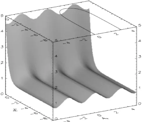
[image:30.595.186.395.479.702.2]

component in they-direction makes the field force-free, since B2 = B_x2 +B_y2 = B₀2. Figure 1.4(from Harrison, 2009) shows a plot of the field lines for the force-free Harris sheet. Using

(31)

Amp`ere’s law (Equation (1.33)), the current density is given by

j_{f f hs} = B0

µ0L

1 cosh(z/L)

tanh(z/L), 1

cosh(z/L),0

, (1.54)

and so it can be seen thatj×B= 0, as is required for a force-free field. The magnetic pressure is given by

B2

2µ0

= B

2

x+By2

2µ0

= B

2 0

2µ0

, (1.55)

which is constant, and so the plasma pressure is given by

P =Ptotal−Pmagnetic=constant. (1.56)

It is they-component of the field, therefore, which maintains the force balance across the sheet, since both the plasma and magnetic pressure are constant, but the magnetic field itself varies with

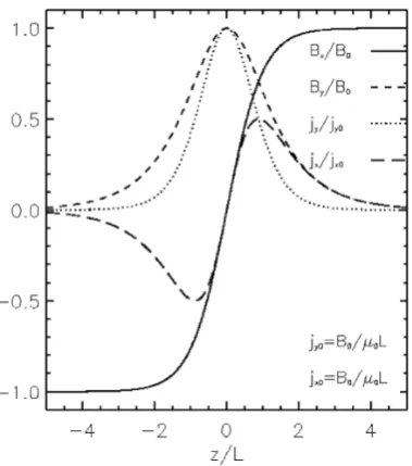
[image:31.595.194.384.404.619.2]

z. Figure1.5(fromHarrison,2009) shows normalised magnetic field and current density profiles for the force-free Harris sheet.

Figure 1.5: Plot of normalised magnetic field, current density and pressure profiles for the force-free Harris sheet (fromHarrison,2009).

As the magnetic field (1.53) is force-free, the current density is parallel to the magnetic field,

j_{f f hs}= α(z)

µ0

(32)

with the force-free parameterα(z)given by

α(z) = 1

L

1

cosh(z/L), (1.58)

which varies withz, meaning that the force-free Harris sheet field is a nonlinear force-free field.

As previously discussed, this means thatα is constant along a given field line, but varies from field line to field line.

1.4.2 Vlasov-Maxwell Equilibria

Vlasov-Maxwell equilibria can be found by solving the steady-state Vlasov equation,

v·∂fs

∂r +

qs

ms

(E+v×B)·∂fs

∂v = 0, (1.59)

together with the steady-state Maxwell equations,

∇ ·E = σ

0

, (1.60)

∇ ×E = 0, (1.61)

∇ ×B = µ0j, (1.62)

∇ ·B = 0. (1.63)

Throughout the work in this thesis, it is assumed that each equilibrium quantity varies only with thez-coordinate, so that there is spatial invariance with respect to thex- andy-coordinates.

Fur-thermore, it is assumed that the magnetic field vanishes in thez-direction, and can be written as

B=∇ ×A, whereA= (Ax, Ay,0)is a vector potential whosez-component can be assumed to vanish without loss of generality. This assumption ensures that Equation (1.63) is automatically

satisifed. Thex- andy-components ofBare then given by,

Bx = −

dAy

dz , (1.64)

By =

dAx

dz , (1.65)

It is also assumed that the electric fieldEcan be written asE=−∇φ, whereφis a scalar potential, so that

Ez =−

dφ

dz, (1.66)

(33)

As discussed in Section1.3.1, quasineutrality can be assumed ifL, the typical length scale of the

plasma, is much larger than the Debye length,λD. Note, however, that this does not imply that the electric field vanishes (Harrison and Neukirch,2009a).

Due to the symmetries of the system. there are three constants of motion, namely the Hamiltonian Hs, arising from the time independence of the system, given by

Hs=

1 2ms(v

2

x+vy2+v2z) +qsφ, (1.67) the canonical momentum in thex-direction, arising from the spatial symmetry in thex-direction, given by

pxs =msvx+qsAx, (1.68)

and the canonical momentum in the y-direction, arising from the spatial symmetry in the y -direction, given by

pys=msvy +qsAy. (1.69)

The steady-state Vlasov equation (1.59) is satisfied by positive functions (distribution functions)

fs=fs(Hs, pxs, pys), which depend only on the constants of motion.

The remaining two Maxwell equations to be solved are Gauss’ law (Equation (1.60)) and Amp`ere’s law (Equation (1.62)), the components of which can be expressed as

−0

d2φ

dz2 = σ, (1.70)

− 1

µ0

d2Ax

dz2 = jx, (1.71)

− 1

µ0

d2Ay

dz2 = jy, (1.72)

where, as was discussed in Section1.3.1, the charge densityσand thex- andy-components of the

current density,jxandjy, can be expressed as moments of the distribution functions as follows,

σ(Ax, Ay, φ) =

X

s

qs

Z ∞

−∞

fs(Hs, pxs, pys)d3v, (1.73)

jx(Ax, Ay, φ) =

X

s

qs

Z ∞

−∞

vxfs(Hs, pxs, pys)d3v, (1.74)

jy(Ax, Ay, φ) =

X

s

qs

Z ∞

−∞

vyfs(Hs, pxs, pys)d3v. (1.75)

(34)

densities satisfy the following relations

∂σ ∂Ax

+∂jx

∂φ = 0, (1.76)

∂σ ∂Ay

+∂jy

∂φ = 0, (1.77)

∂jx

∂Ay − ∂jy

∂Ax

= 0, (1.78)

and also that, for a quasineutral plasma, the components of the current density can be expressed as

jx(Ax, Ay, φ) =

∂Pzz

∂Ax

, (1.79)

jy(Ax, Ay, φ) =

∂Pzz

∂Ay

, (1.80)

(see alsoGrad,1961;Bertotti, 1963;Lerche,1967;Channell,1976;Mynick et al.,1979;Attico and Pegoraro,1999). Additionally, the charge densityσcan be written as

σ(Ax, Ay, φ) =−

∂Pzz

∂φ , (1.81)

(e.g.Bertotti, 1963;Lerche, 1967;Mynick et al., 1979). In Equations (1.79)-(1.81),Pzz is the

zz-component of the pressure tensor, defined in terms of the distribution functions as

Pzz =

X

s

ms

Z

v_z2fsd3v. (1.82)

Note that there is no drifting of particles in thez-direction, and so the above definition of Pzz is consistent with the general definition of the pressure tensor, given in Equation (1.9). Using Equations (1.79) and (1.80), Amp`ere’s Law (Equations (1.71) and (1.72)) can then be written in

terms of the vector potential,A, and the pressure,Pzz, which gives

d2Ax

dz2 =−µ0

∂Pzz

∂Ax

, (1.83)

d2Ay

dz2 =−µ0

∂Pzz

∂Ay

. (1.84)

The scalar potentialφcan be determined from the quasineutrality conditionne = ni, which, to lowest order, corresponds to the condition

∂Pzz

∂φ = 0, (1.85)

(35)

Equa-1.4 Plasma Equilibria 20

Particle Motion 1D VM Equilibrium

time:t coordinate:z

position:x,y vector potential:Ax,Ay potential:V(x, y) pressure:µ0Pzz(Ax, Ay)

energy:m(v2_x+v_y2)/2 +V(x, y) total pressure:(B_x2+B2_y)/2µ0+Pzz equations of motion: Amp`ere’s law:

d2x

dt2

=

−

∂V

∂x

d2Ax

dz2

=

−

µ

0 ∂Pzz

∂Ax d2y

dt2

=

−

∂V

∂y

d2Ay

dz2

=

−

µ

0 ∂Pzz

∂Ay

Table 1.2: The analogy between the one-dimensional Vlasov-Maxwell equilibrium problem and the problem of solving the equations of motion of a particle in a two-dimensional conservative potential.

tions (1.83) and (1.84) for the pressurePzz, which can then be used to determine the distribution function (by using the definition (1.82) ofPzz).

Integrating Amp`ere’s Law gives the force balance condition

B2

2µ0

+Pzz =PT, (1.86)

wherePT is a constant. This condition states that the sum of the plasma and magnetic pressures across the sheet must be constant. Note that other components of the pressure tensor could be

calculated by taking different moments of the distribution function, but they are not important for the force balance and so will not be considered.

Solving Equations (1.83) and (1.84) for the pressurePzz is analogous to solving the equations of motion of a particle in a two-dimensional conservative potential, as has been noticed by a number of authors (e.g.Grad,1961;Sestero,1966;Lam,1967;Parker,1967;Lerche,1967;Alpers,1969;

Su and Sonnerup,1971;Kan,1972;Channell, 1976;Mynick et al.,1979;Lee and Kan, 1979b;

Greene,1993;Attico and Pegoraro,1999;Harrison and Neukirch,2009a), withztaking the role of time,AxandAy the coordinates of the particle andµ0Pzz the potential. Table1.2summarises this analogy, with the quantities and equations from the particle problem given on the left-hand

side, and the equilibrium quantities and equations given on the right-hand side.

In the particle problem, the shape of the potential as a function of position can give insight into

the nature of the particle trajectories. In analogy with this, the shape of the pressurePzz can give information about the nature of the solutions of Equations (1.83) and (1.84). The force balance

condition (1.86) corresponds to the condition of the total energy being constant in the particle

(36)

1.4.2.1 Vlasov-Maxwell Equilibrium for the Harris Sheet

The Harris sheet model was discussed in Section1.4.1.1in the MHD context. It can also be

rep-resented in Vlasov theory, as described byHarris(1962). Listed again for reference, the magnetic field is given by

BHarris =B0(tanh(z/L),0,0), (1.87)

whereB0is a constant andLis a parameter which specifies the thickness of the sheet. The vector

potential is given by

AHarris =B0L(0,−ln[cosh(z/L)],0), (1.88)

and solving Amp`ere’s law (1.62) gives the current density as

j_Harris= B0

µ0L

0, 1

cosh2(z/L),0

. (1.89)

Thezz-component of the pressure tensor,Pzz,Harris, is given, as a function ofz, by

Pzz,Harris=

B2₀

2µ0

1

cosh2(z/L)+Pb,zz, (1.90)

wherePb,zzis a constant background pressure. This expression is the same as in the MHD context. Using the fact thatcosh(z/L) = exp(−Ay/B0L) (from equation (1.88)) gives the pressure in

terms ofAxandAy as

Pzz(Ax, Ay) =

B2 0

2µ0

exp

2Ay

B0L

+Pb,zz. (1.91)

A solution of the steady-state Vlasov equation (1.59) for this magnetic field profile was obtained

byHarris(1962), and is given by

fs,Harris=

n0s

(√2πvth,s)3

exp[−βs(Hs−uyspys)], (1.92)

whereuys is a constant average bulk flow velocity in they-direction. Force balance across the sheet is maintained by a pressure gradient - since the magnetic pressure varies withzso must the

plasma pressure in order to maintain force balance.

(37)

1.5 Aims and Outline of Thesis 22

Fu and Hau(2005), which is a kappa-type distribution function of the form

fs,f u =

n0

2πv2

th,s

Γ(κ+ 1) Γ(κ−1

2)κ3/2

"

1 + 1 2κv2

th,s

[c2₁_s+ (c2s−us)2+c23s]

#−(κ+1)

, (1.93)

whereΓis the gamma function (e.g.Abramowitz and Stegun,1964), andc1s,c2sandc3sare the constants of motion, which are given by

c1s =

v2_z−2qs

ms

Ayvy−

q2_s m2

s

A2_y

1/2

, (1.94)

c2s = vy+

qs

ms

Ay =

pys

ms

, (1.95)

c3s = vx=

pxs

ms

. (1.96)

It will be seen in Sections2.7and2.8 that different distribution functions can also be found for

the force-free Harris sheet, in addition to the known solution found byHarrison and Neukirch

(2009b).

1.5 Aims and Outline of Thesis

The aims of this thesis can be summarised as follows:

1. Investigate in detail the properties of the known nonlinear one-dimensional force-free

Vlasov-Maxwell equilibrium found byHarrison and Neukirch(2009b).

2. Find other one-dimensional force-free Vlasov-Maxwell equilibria.

3. Carry out a linear stability analysis of Harrison and Neukirch’s equilibrium distribution

function.

Aim 1 is motivated by the fact that the distribution function found by Harrison and Neukirch

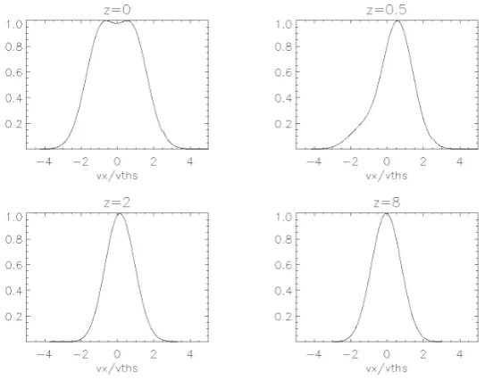
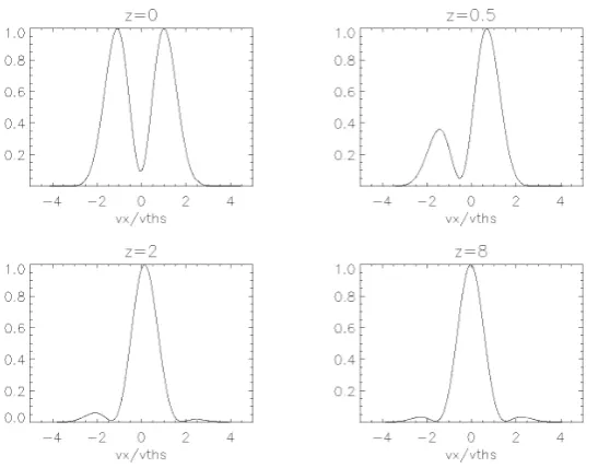
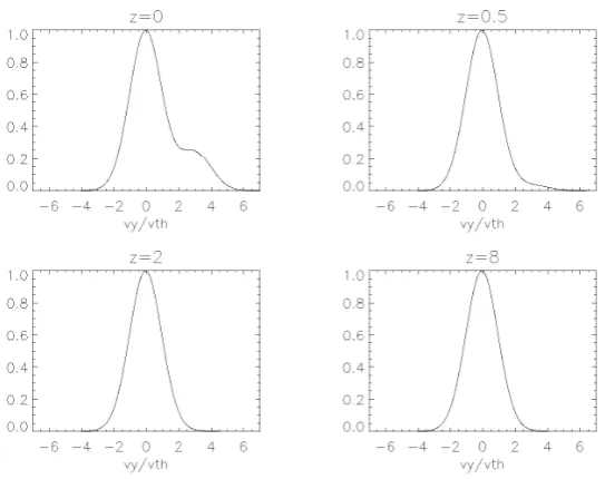
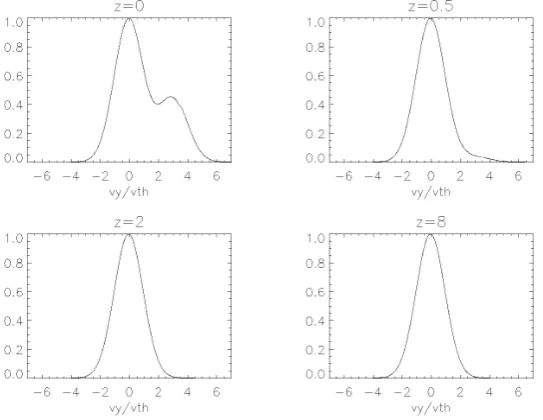
(2009b) can be multi-peaked in both thevx- and vy-directions. This is of interest, since such a distribution function may give rise to microinstabilities (e.g.Krall and Trivelpiece,1973), in ad-dition to macroscopic instabilities, such as the collisionless tearing mode (e.g.Schindler,2007). Conditions on the parameters of the distribution function are given, which show when the distri-bution function can be single or multi-peaked. It should be noted, however, that an investigation

into the microinstabilities themselves is beyond the scope of this thesis.

(38)

for particle-in-cell (PIC) simulations of collisionless reconnection. At present, in order to mimic

a force-free field, a constant guide field is added to the Harris sheet field (Harris, 1962). This approach gives a current density which is partially field aligned, but increasing the strength of the

guide field does not change the strength of the current density, and so no free energy is added to

the system. When starting with a proper force-free equilibrium, the strength of the current density and, hence, the available free energy, are coupled to the shear of the magnetic field. In addition,

the plasma density and pressure are constant, which is not true in the guide field case. Harrison

(2009) has carried out the first PIC simulations for the force-free Harris sheet, using theHarrison and Neukirch(2009b) distribution function as initial conditions. Although these simulations were preliminary, they hinted at possible significant differences to simulations using the Harris sheet plus guide field as initial conditions. PIC simulations will not be considered in this thesis, but it is

important to note that finding further force-free distribution functions would give a bigger range

of possible initial conditions, and thus may lead to a deeper understanding of the collisionless reconnection process in the future.

There are three separate parts which can all be categorised under aim 2. Firstly, a discussion will

be given of attempts to use the method ofHarrison and Neukirch(2009b) to look for equilibria for other nonlinear force-free field profiles. It will be shown, however, that even for seemingly simple

field profiles, this method is unsuccessful. A new method was required, therefore, which led,

secondly, to the discovery of a family of distribution functions for the force-free Harris sheet field profile, which includes the known solution found byHarrison and Neukirch (2009b). Thirdly, an attempt has been made to extend the theory of the one-dimensional equilibrium problem to

cylindrical coordinates, and to find a distribution function for a one-dimensional flux tube, by considering the case where all quantities depend only upon the radial coordinate,r. This attempt,

however, did not lead to a force-free equilibrium.

As stated above, the Harrison and Neukirch equilibrium may give rise to macroscopic instabilities,

such as the collisionless tearing mode. This is the motivation for aim 3. A central difficulty in such

a stability analysis, however, is that the Vlasov equation must be integrated over the unperturbed particle orbits, and so an expression for the orbits is required. This is, in general, not possible to

do exactly analytically and so, in order to make analytical progress, it will be necessary to use

an approximation for the force-free Harris sheet field profile, in addition to a number of other approximations.

The work in this thesis is laid out as follows: in Chapter 2, the focus is one-dimensional

force-free Vlasov-Maxwell equilibria, with a detailed discussion of the properties of theHarrison and Neukirch(2009b) equilibrium given, together with a discussion of finding other distribution func-tions, for the force-free Harris sheet and other magnetic field profiles. In Chapter 3, the initial

(39)

(40)

Chapter 2

One-Dimensional Force-Free Vlasov-Maxwell

Equilibria

Parts of the work in the present chapter have been adapted fromNeukirch, Wilson, and Harrison

(2009) andWilson and Neukirch(2011).

2.1 Introduction

Investigations of plasma instabilities and plasma waves frequently start with a consideration of

equilibrium solutions of the governing equations. In the MHD picture, as was discussed in

Sec-tion1.4.1, equilibria can be found by solving the equations of magnetohydrostatics (MHS) (e.g.

Neukirch, 1998). When using kinetic theory, and assuming that the plasma is collisionless, the required equilibria can be found by solving the steady-state Vlasov-Maxwell equations (e.g.Krall and Trivelpiece,1973). The general theory of one-dimensional Vlasov-Maxwell equilibria was discussed in Section1.4.2.

The work in the present chapter will focus on one-dimensional force-free Vlasov-Maxwell

equi-libria. Force-free fields, for whichj×B= 0, such that the current density and magnetic field are parallel to each other, are useful for modelling low-beta plasmas such as that of the solar corona.

Finding collisionless distribution functions for such field profiles is, however, a highly non-trivial

task. This is reflected in the fact that there are relatively few known examples. Of these known ex-amples, only one is of the nonlinear force-free type (Harrison and Neukirch,2009b), with the rest being linear force-free (Sestero,1967;Channell,1976;Bobrova and Syrovatskiˇi,1979;Bobrova et al.,2001).

Harrison and Neukirch(2009a) have discussed conditions for the existence of one-dimensional force-free solutions of the Vlasov-Maxwell equations. Usingj = (∇ ×B)/µ0, the force-free

condition for a one-dimensional model is given by

d dz

B2

2µ0

= 0, (2.1)

(41)

2.1 Introduction 26

which states that the magnetic pressure must be constant. The force-balance condition (1.86) then

implies that the plasma pressure,Pzz, must also be constant. As discussed in Section1.4.2, thex -andy- components of the current density can be written as partial derivatives ofPzzwith respect toAxandAy (See Equations (1.79) and (1.80)). The force-balance condition would then appear to imply that the current density must also vanish for a force-free equilibrium. This condition, however, only implies thatPzz is constant as a function ofz, and so it can still vary with respect to the vector potential. The condition gives

dPzz

dz = ∂Pzz

∂Ax

dAx

dz + ∂Pzz

∂Ay

dAy

dz = 0, (2.2)

and so it is clear that this condition can be satisfied even if the partial derivatives are non zero.

This is an important property of one-dimensional force-free equilibria (Harrison and Neukirch,

2009a).

Returning to the particle analogy, which was discussed in Section1.4.2, the condition (2.2) means that the pressurePzz must have at least one contour which is also a particle trajectory in theAx

-Ay-plane, in order to allow a particle trajectory to be obtained that corresponds to a force-free field. As stated byHarrison and Neukirch(2009a), this is a necessary condition for the existence of a force-free Vlasov-Maxwell equilibrium. So, starting with a magnetic field profile, a first

step is to calculate the vector potentialA, then to use Amp`ere’s law to find the pressure Pzz. A surface plot of Pzz in the Ax-Ay plane with the trajectory of Aoverplotted should then reveal that the trajectory is a contour of the pressure. This will be illustrated further in Sections2.2and

2.4, where the previously known force-free solutions will be discussed (Sestero,1967;Channell,

1976;Bobrova and Syrovatskiˇi,1979;Bobrova et al.,2001;Harrison and Neukirch,2009b).

It is also noted byHarrison and Neukirch(2009a) that a well known family of potentials, attractive central potentials, allow trajectories which are contours of the potential. These potentials have

circular contours, and allow circular particle trajectories. The known linear force-free solutions (Sestero,1967;Channell,1976;Bobrova and Syrovatskiˇi,1979;Bobrova et al.,2001) give rise to such potentials, which will be discussed further in Section2.2.

Once the pressure functionPzz is known, the solution to the Vlasov-Maxwell equations can be completed by finding a distribution function fromPzz. One way of doing this is to start with the definition (1.82) of the pressure and solve an integral equation for the distribution function. An illustration of this method has been given byChannell(1976), which will be discussed further in Section2.3. Channell’s method was used byHarrison and Neukirch(2009b) to find a distribution function for the force-free Harris sheet. This was the first non-linear force-free Vlasov-Maxwell equilibrium to be found, and has a number of interesting properties. In particular, the distribution

(42)

2.2 A Linear Force-Free Vlasov-Maxwell Equilibrium 27

to present a detailed discussion of the properties of this equilbrium, and to give conditions on

the parameters which show when the distribution function can be single or multi-peaked. The derivation of the distribution function will be given in Section2.4, and the conditions to ensure

several maxima will be discussed in Section2.5.

In Section 2.6, a discussion is given of attempts to use the method of Harrison and Neukirch

(2009b) to find Vlasov-Maxwell equilibria for other magnetic field profiles. It will be shown that it is difficult to successfully use this method, even for seemingly simple magnetic field profiles. It seems, therefore, that the force-free Harris sheet is one of the few field profiles for which the

method can be used successfully. Although these attempts were unsuccessful, another method was

developed which allows a family of distribution functions to be found for the force-free Harris sheet, by using properties of the pressurePzz. This method will be discussed in Sections2.7and 2.8.

It is also remarked byChannell (1976) that a straightforward extension of the one-dimensional force-free equilibrium problem to cylindrical coordinates is not possible. This will be discussed

further in Section 2.9, and an example will be given of an attempt to find a linear force-free

distribution function for one-dimensional flux tubes, by considering the case where all quantities depend only on the radial coordinate,r.

2.2 A Linear Force-Free Vlasov-Maxwell Equilibrium

As discussed byHarrison and Neukirch(2009a), the previously known linear force-free solutions (Sestero,1967;Bobrova and Syrovatskiˇi,1979;Bobrova et al.,2001) have a distribution function of the form

fs =

n0s

v3

th,s

exp

−βsHs−

βsas

ms

(p2_xs+p2_ys)

, (2.3)

where it should be noted that the scalar potentialφ vanishes as a result of the quasineutrality

condition. The distribution function (2.3) gives rise to a pressure of the form

Pzz = P0exp[−r(A2x+A2y)], (2.4) where P0 and r are constants (note that r must be negative so that the pressure Pzz given by Equation (2.4) represents an attractive central potential). Using Equations (1.79) and (1.80) gives

Amp`ere’s law (Equations (1.83) and (1.84)) as

d2Ax

dz2 = 2µ0P0rAxexp[−r(A 2

(43)

d2Ay

dz2 = 2µ0P0rAyexp[−r(A 2

x+A2y)], (2.6)

which has solutions of the form

Ax = ksinαz, (2.7)

Ay = kcosαz, (2.8)

and so, using Equations (1.64) and (1.65), the magnetic field profile is given by

Bx = kαsinαz, (2.9)

By = kαcosαz. (2.10)

It is clear thatB_x2+B2_y =k2α2 =constant, and so the field is a linear force-free field. This can also be seen by looking at the current density, which has the form

jx = −2P0rAxexp[−r(A2x+A2y)], (2.11)

jy = −2P0rAyexp[−r(A2x+A2y)], (2.12) which can be written asj=αB, where

α=p(−2rP0) exp

₋

rk2

2

, (2.13)

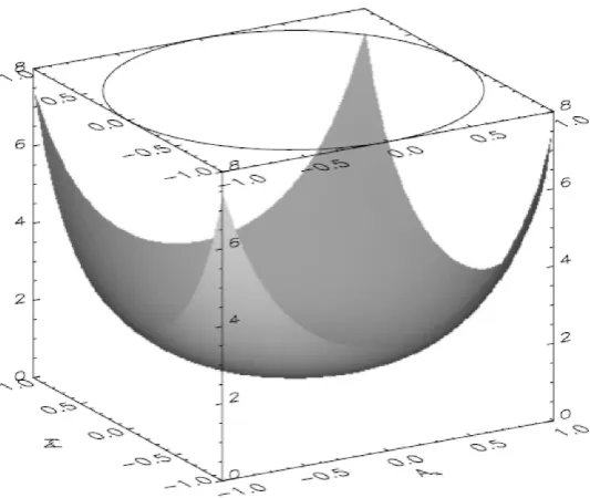
which is constant with respect toz, as is required for a linear force-free field. Note that the square

root in Equation (2.13) gives a real number, sincer <0. Figure2.1(fromHarrison,2009) shows a surface plot of the pressure (2.4) in theAx-Ay-plane, with the solutions (2.7) and (2.8) plotted as a trajectory at the top. This figure reveals that the solution forAis clearly a contour of the potential, which illustrates the fact that this must be true for a linear force-free solution.

Another example of a distribution function that gives rise to the linear force-free magnetic field components (2.9) and (2.10) has been given byChannell(1976) andAttico and Pegoraro(1999) as

fs(Hs, pxs, pys) = exp(−βsHs)(F0s+F1s(p2xs+p2ys)), (2.14) whereF0sandF1sare constants. This distribution function results from aPzz of the form

Pzz =P00+

1 2P01(A

2

x+A2y), (2.15)

(44)

[image:44.595.164.431.113.338.2]

Figure 2.1: Surface plot ofPzz over theAx-Ay-plane for the linear force-free solution described bySestero(1967);Bobrova and Syrovatskiˇi(1979);Bobrova et al.(2001). The solutions (2.7) and (2.8) are plotted as a trajectory at the top of the plot, showing thatAis a contour of the pressure (fromHarrison,2009).

second order ODEs,

−d

2_A

x

dz2 = P01Ax, (2.16)

−d

2_A

y

dz2 = P01Ay, (2.17)

which can be solved to give the components of the vector potential as

Ax = Ax0sin(

p

P01z+δx), (2.18)

Ay = Ay0sin(

p

P01z+δy). (2.19)

As noted byHarrison and Neukirch(2009a), choosingAx0 =Ay0 = k,δx = 0,δy =π/2and √

P01=αgives the solutions (2.7) and (2.8).

It has also been shown by Harrison and Neukirch(2009a) that all distribution functions of the form

fs=fs(Hs, p2s), (2.20) wherep2

(45)

2.3 Channell’s Method for Finding Force-Free Vlasov-Maxwell Equilibria 30

the linear force-free field components (2.9) and (2.10).

For nonlinear force-free solutions, the potential cannot be an attractive central potential, but must still have a contour which is also a particle trajectory (Harrison and Neukirch,2009b). This will be discussed further in Section2.4.

2.3 Channell’s Method for Finding Force-Free Vlasov-Maxwell

Equi-libria

For a known distribution function, thezz-component of the pressure tensor,Pzz, can be calculated directly through the definition (1.82). Amp`ere’s law in the form given by Equations (1.71) and (1.72) can then be used to determine the magnetic field profile. If the aim is to find a distribution

function corresponding to a given magnetic field profile, however, then the problem must be solved

in the inverse direction. This is a natural way to solve the problem for force-free fields, since the magnetic field is restricted by the conditionj×B= 0.

Such a method for finding force-free Vlasov-Maxwell equilibria has been suggested byChannell

(1976). It is assumed, firstly, that the distribution functions have the form

fs=

n0s

(√2πvth,s)3

exp(−βsHs)gs(pxs, pys), (2.21)

wheregs is an arbitrary function of the canonical momenta andβs = 1/(kBTs), withkB equal to the Boltzmann constant. The pressure,Pzz, resulting from this arbitrary distribution function is given, using the definition (1.82), by

Pzz =

X

s

1

βs

exp(−βsqsφ)Ns(Ax, Ay), (2.22)

whereNsis given by

Ns(Ax, Ay) =

n0s

2πv_th,s2

Z ∞

−∞

Z ∞

−∞

exp

−βsms

2 (v

2

x+vy2)

×gs(pxs, pys)dvxdvy. (2.23)

The quasineutrality condition means, to lowest order, that the charge density, σ = −∂Pzz/∂φ, vanishes, which gives

σ(Ax, Ay, φ) =

X

s

(46)

2.3 Channell’s Method for Finding Force-Free Vlasov-Maxwell Equilibria 31

Summing over particle species (ions and electrons) and solving for the quasineutral electric

po-tential,φqn, then gives

φqn=

1

e(βe+βi)

ln

Ni

Ne

. (2.25)

It can be seen that settingNe = Ni = N gives φqn = 0. This corresponds to strict charge neutrality, since settingφ = 0 in Equation (2.22) means that Ns gives the number density of speciess. In order to satisfy the condition of strict charge neutrality, certain conditions will have

to be imposed on the various parameters in the distribution function, which can be determined once the full expression is known.

Substituting the quasineutral electric potential (2.25) into Equation (2.22) gives the quasineutral

pressure,Pzz,qn, as

Pzz,qn(Ax, Ay) =

βe+βi

βeβi

N(Ax, Ay), (2.26) and Equation (2.23) can then be rewritten as

n0s

2πm2

svth,s2

Z ∞

−∞

Z ∞

−∞

exp

− βs

2ms

[(pxs−qsAx)2+ (pys−qsAy)2]

×gs(pxs, pys)dpxsdpys=

βeβi

βe+βi

Pzz,qn(Ax, Ay), (2.27) where the integration has been written over the canonical momenta instead ofvxandvy. Equation (2.27) is a Fredholm integral equation of the first type (e.g.Moiseiwitsch,1977), which must be solved for the functiongs. This integral equation has the kernel

K(pxs, pys;qsAx, qsAy)∝exp

− βs

2ms

(pxs−qsAx)2+ (pys−qsAy)2

, (2.28)

which depends only on the difference of its arguments, and so the double integral in Equation

(2.27) is of convolution type. Such an integral equation can be solved by using Fourier transforms, as suggested byChannell(1976). This is useful, as it allows the double integral to be dealt with without actually doing the integration directly.

Channell’s method works for the Force-Free Harris sheet model (Harrison and Neukirch,2009a;

Neukirch, Wilson, and Harrison,2009), but for other pressure profiles, resulting from seemingly simple nonlinear force-free magnetic fields, it does not work (see Section2.6for a further

discus-sion of this point). In order for the method to work, the Fourier transform ofPzz must exist, and the inverse Fourier transform of the resulting function must also exist, from which the function

(47)

in-2.4 Force-Free Harris Sheet - Harrison and Neukirch Equilibrium 32

verse of the exponential term in the double integral of Equation (2.27)). It seems, therefore, that

Channell’s Fourier transform method will only work for a few specially selected magnetic field profiles. Channell does, however, discuss other examples for which the Fourier transform method

does not work.

In the next section, a derivation of the Harrison and Neukirch distribution function for the

force-free Harris sheet will be given (Harrison and Neukirch,2009a;Neukirch, Wilson, and Harrison,

2009). Although Fourier transforms do work for this particular field profile, they will not be used in the derivation, since they are of limited applicability, as will be demonstrated further in Section

2.6.

2.4 Force-Free Harris Sheet - Harrison and Neukirch Equilibrium

The force-free Harris sheet equilibrium is straightforward in MHD, as demonstrated in Section

1.4.1.2. In Vlasov theory, however, finding distribution functions from the magnetic field profile is a non-trivial task. In the present section, a derivation will be given of the distribution function

found by Harrison and Neukirch (Harrison and Neukirch,2009b;Neukirch, Wilson, and Harrison,

2009).

The magnetic field of the force-free Harris sheet is given by

Bx,f f hs = B0tanh(z/L), (2.29)

By,f f hs =

B0

cosh(z/L), (2.30)

withBz,f f hs = 0. Using Equations (1.64) and (1.65) gives the non-vanishing components of the vector potential as

Ax,f f hs = 2B0Ltan−1(ez/L), (2.31)

Ay,f f hs = −B0Lln cosh(z/L). (2.32)

The non-vanishing components of the current density are given by

jx,f f hs =

B0

µ0L

sinh(z/L)

cosh2(z/L), (2.33)

jy,f f hs =

B0

µ0L

1

cosh2(z/L). (2.34)

Equilibrium and stability properties of collisionless current sheet models

EQUILIBRIUM AND STABILITY PROPERTIES OF

COLLISIONLESS CURRENT SHEET MODELS

Fiona Wilson

A Thesis Submitted for the Degree of PhD

at the

University of St Andrews

2013

Full metadata for this item is available in

Research@StAndrews:FullText

at:

http://research-repository.st-andrews.ac.uk/

Please use this identifier to cite or link to this item:

http://hdl.handle.net/10023/3548

This item is protected by original copyright

Equilibrium and Stability Properties of

Collisionless Current Sheet Models

Fiona Wilson

Abstract

Declarations

Publications

Acknowledgements

Contents

Introduction

1.1

Background

1.2

Definition of a Plasma

1.3

Plasma Models

1.4

Plasma Equilibria

=

−

=

−

µ

=

−

=

−

µ

1.5

Aims and Outline of Thesis

One-Dimensional Force-Free Vlasov-Maxwell

Equilibria

2.1

Introduction

2.2

A Linear Force-Free Vlasov-Maxwell Equilibrium

2.3

Channell’s Method for Finding Force-Free Vlasov-Maxwell

Equi-libria

2.4

Force-Free Harris Sheet - Harrison and Neukirch Equilibrium