An Improved Analytical Model for IEEE 802 11 Distributed Coordination Function under Finite Load

An Improved Analytical Model for IEEE 802.11

Distributed Coordination Function under Finite Load

Rama Krishna CHALLA1, Saswat CHAKRABARTI2, Debasish DATTA3

1_{Department of Computer Science, National Institute of Technical Teachers’ Training and Research, Chandigarh, India} 2_{G. S. Sanyal School of Telecommunications, Indian Institute of Technology, Kharagpur, India}

3_{Department of Electronics and Electrical Communication Engineering, Indian Institute of Technology, Kharagpur, India}

Email: [email protected], rkc_97@yahoo.com

Received November 27, 2009; revised March 26, 2009; accepted March 29, 2009

ABSTRACT

In this paper, an improved analytical model for IEEE 802.11 distributed coordination function (DCF) under finite load is proposed by closely following the specifications given in IEEE 802.11 standard. The model is investigated in terms of channel throughput under perfect and slow Rayleigh fading channels. It is shown that the proposed model gives better insight into the operation of DCF.

Keywords: IEEE 802.11, Markov, DCF, Wireless LANs, Backoff, Perfect Channel, Rayleigh Fading

Channel, Saturation, Finite Load, Throughput

1. Introduction

IEEE 802.11 has been standardized and widely adopted for wireless local area networks (WLANs) [1]. In this standard, it specifies two fundamental access mecha-nisms, i.e., point coordination function (PCF) and dis-tributed coordination function (DCF). Since IEEE 802.11 DCF mechanism supports adhoc networking configura-tion and has been widely adopted in wireless networks, we focus our analysis only on this mechanism. DCF mechanism is based on the carrier sense multiple access with collision avoidance (CSMA/CA) protocol. In DCF, data frames are transmitted via two mechanisms, i.e., basic access mechanism and request-to-send/clear-to- send (RTS/CTS) mechanism.

Performance analysis of DCF has been reported in several research works through either simulation or mathematical modeling [2-13]. The Markov model pro-posed in [2] for IEEE 802.11 DCF has gained wide ac-ceptance due to its simplicity. However, it exhibits some constraints according to [1]. First, the model is limited to deriving the saturation throughput. It excludes the per-formance analysis under finite load condition, which is an important practical scenario in a WLAN. Secondly, it does not take into account the loss of frames due to channel contention. This frame loss has been shown to

be significant in [10]. Finally, decrementing a backoff value by a station (STA) is not modeled correctly as per 802.11 standard [1].

How-ever, in all the proposed models, decrementing a backoff value by an STA is not correctly modeled according to [1]. As per the standard [1], an STA in any backoff stage should decrement its backoff counter value only when the channel status is found to be idle for at least DCF inter-frame space (DIFS) duration. Whereas in the pro-posed models, an STA decrements its backoff counter value irrespective of the channel status i.e., whether the channel is busy or idle, which is not complying with [1]. In this work, we follow the models in [2,14]. Hereafter, we refer to model in [2] as Bianchi's model and model in [14] as Pham's model. Readers are requested to refer [1] for a detailed discussion on IEEE 802.11 DCF operation.

In this paper, we propose an improved Markov model for IEEE 802.11 DCF under finite load by closely fol-lowing the specifications in [1]. The model is investi-gated in terms of channel throughput under perfect and slow Rayleigh fading channels for different packet arri-val rate and number of STAs in the network.

The rest of the paper is organized as follows: Section 2 describes the proposed Markov model for IEEE 802.11 DCF under finite load, followed by the performance analysis for perfect channel conditions. The model de-veloped in Section 2 is extended for a slow Rayleigh fading channel and the performance is analyzed in Sec-tion 3. Finally SecSec-tion 4 presents the concluding remarks on the work.

2. Markov Model for IEEE 802.11 DCF

As discussed above, the Markov models presented in literature have shortcomings. Complementing the work in [2,14], we focus on the performance analysis of IEEE 802.11 DCF under finite load condition. The saturation throughput considered in [2] is just one par-ticular case of our analysis. We divide our contribution into two parts. In the first part, we propose an im-proved Markov model for DCF assuming perfect channel conditions. Next, we extend this model for a slow Rayleigh fading channel. For simplicity, we use the same notation as given in [14].

2.1.

Proposed Markov Model for IEEE 802.11 DCF

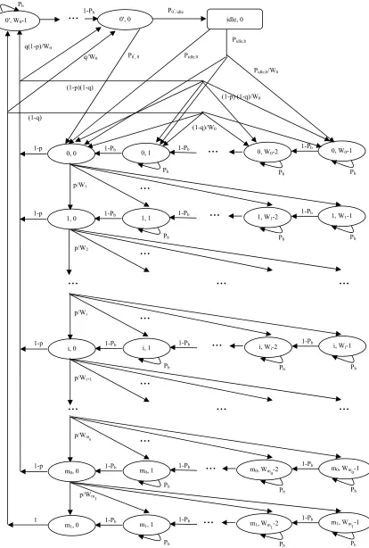
Let be the number of stations (STAs) in a WLAN contending for channel access. Let and be the stochastic processes representing the backoff counter and number of the backoff stages respectively. The backoff states and its transition probabilities for a given STA are shown in Figure 1. The parameters used in our model are described in Table 1. We assume that the channel is perfect (i.e., error free) and the packets are lost only due to collisions.

n

) (t

b s(t)

Under saturation condition, an STA always has a packet for transmission in its queue. Therefore, it enters straight away to state S0,k, . However, un-der finite load, if the STA’s queue is empty, the station enters into one of the states ,

1 0kW0

k

S0, 0kW01, oth-erwise the STA enters one of the backoff states S0,k,

1 0kW0

0

. At state S0',0, if there is a packet for transmission, the STA starts transmitting the packet by moving to the state S0,0 with probability P0',0. Otherwise, the STA enters the state Sidle,0 with probability P0',idle. At state Sidle,0 once a frame arrives into the queue of a STA and if the channel has been found to be idle for more than DIFS, this frame is transmitted immediately with probability Pidle,0. Otherwise, the STA goes to backoff state S0,k, kW01 with probability Pidle,b.

The state of each STA is described by , where indicates the current backoff stage, 1

) , (i k b

m i

i 0  and k

is the backoff counter value measured in time slots,

[image:2.595.308.539.347.720.2]

1 0kW_i .

Table 1. Summary of parameters.

Pb Probability that an STA in the backoff stage_{senses the channel busy}

p Probability of a packet not received successfully Wi Backoff window size at stage s(t)=i

W0 Minimum backoff window size

q Probability that the queue is empty

b(i, j) Probability of an STA in the backoff state Si,j

b(idle, 0) Stationary probability at idle state Sidle,0 Sidle,0 Channel is in idle state

τ Probability of STA transmitting a packet Si,j State of STA when s(t)=i and b(t)=j

λ Average packet arrival rate

P0',0 Transition probability from state S0',0 to S0,0 Pidle,0 Transition probability from state Sidle,0 to S0,0 Pidle,b Transition probability from state _{off state} Sidle,0 to

back-P0',idle Transition probability from state S0',0 to Sidle,0 Ptr (n) Probability of at least one out of n STAs transmit

Ps(n) Probability of successful transmission for _STAs n

 Average slot time s

 Average slot time at saturation Usta Channel throughput per station Utotal Total normalized channel throughput

Ql Queue length eff

 _{Effective packet service rate}

succ

 Rate of successful transmissions disc

 Rate at which packets are being discarded Pdisc Probability that the packet is discarded

ρ Traffic intensity

σ Channel idle slot

_P

b

[image:3.595.95.509.90.704.2]

...

Figure 1. Two dimensional Markov chain for IEEE 802.11 DCF backoff mechanism.

... ...

...

p/Wm 1

...

...

0, W0-1

0, W0-2

0, 0 0, 1 1-Pb

Pb

1-Pb

Pb

Pb

1-Pb

1-p

1, W1-1

1, W1-2

1, 0 1, 1 1-Pb

Pb

1-Pb

Pb

Pb

1-Pb

1-p

p/W1

...

...

p/W2

... ...

...

i, Wi-1

i, Wi-2

i, 0 i, 1 1-Pb

Pb

1-Pb

Pb

Pb

1-Pb

1-p

...

p/Wi

...

...

p/Wi+1

...

p/Wm₀

m0, Wm 0-1

m0, Wm 0-2

m0, 0 m0, 1

1-Pb

Pb

1-Pb

Pb

Pb

1-Pb

1-p

...

m1, Wm₁-1

m1, Wm₁-2

m1, 0 m1, 1

1-Pb

Pb 1-Pb

Pb

Pb

1-Pb

1

...

(1-p)(1-q)

(1-q)

0', 0 0', W0-1

1-Pb P0', idle

idle, 0

q(1-p)/W0

q/W0 P0', 0 Pidle,0

Pidle,b

Pidle,b/W0

(1-p) (1-q)/W0

The Markov chain in Figure 1 is described in the fol-lowing:

1) The backoff counter value is decremented when the STA senses the channel is idle for at least DIFS duration:



, , 1



1 b, 0 1 and 0 i 2

b i k i k  P  i m  k W 

where = is the probability that the channel is found to be busy when at least one of the STAs trans-mits at a given slot time.

b

P _{1(1)}n

2) The backoff counter value is frozen whenever the STA senses that the channel is busy:



, ,



b, 0 1 and 1 i

b i k i k P  i m  k W 1

The above steps (1) and (2) are not included in the ex-isting Markov models.

3) When at least one new frame has arrived at STA’s queue during mandatory backoff stage (i.e., ,

) then

k S0,

1

0kW0 b



0,0 0,0



P0,0.

4) If no frames have arrived during mandatory backoff stage and the STA enters into the IDLE state:



idle



P idle

b ,0 0,0  0,

5) If at least one frame has arrived when an STA is in the IDLE state and the station senses the channel is idle for at least DIFS duration: b



0,0 idle,0



Pidle,0.

6) When at least one frame has arrived and the STA senses the channel is busy:



0, ,0



, 0 0 1

0

, _{  }

 k W

W P idle k

b idleb

7) The frame is not transmitted successfully by an STA in a backoff stage:



, 1,0



 , 1  0,0  i1 i W k m i W p i k i b

8) The frame has been transmitted successfully and there is at least one more packet in the queue of an STA:





                   1 0 , , ) 1 ( 1 0 , 0 , ) 1 ( ) 1 ( 0 , , 0 0 1 0 0 0 0 W k m i W q W k m i W q p i k b

9) The frame is transmitted successfully or lost in col-lision at backoff stage and there is no packet in the queue: th m1





                  1 0 , , 1 0 , 0 , ) 1 ( 0 , , 0 0 1 0 0 0 0 W k m i W q W k m i W p q i k b

Next, we derive the closed-form solution for the pro-posed Markov model. In the steady-state, let



s t i bt k



k i

b(, )tlimPr () , () be the stationary

distribution of the Markov chain. All steady-state prob-abilities are expressed as a function of b(0,0).

We observe that,

1 1 ), 0 , 0 ( ) 0 ,

(i p b i m

b _ i _{ }

(1) Or 1 1 ), 0 , 1 ( ) 0 ,

(i pbi i m

b    

From (1), it is easy to derive the following,



     0 0 1 1 ) 1 ( ) 0 , 0 ( ) 0 , ( m i m p p b i

b (2)

And also, we can find that,

) 0 , 0 ( ) 0 , ( 1

1 p b

m

b _ m

(3) For 1kW_i1, 0im₁, we can derive the following,

) 0 , 1 ( 1 ) , ( _              

 b i

P p W k W k i b b i i (4) when i = k =0, we obtain,

) 0 , ( ) 1 ( ) 0 , ( ) 1 ( ) 1 ( ) 0 , ( ) 0 , ( ) 0 , 0 ( ) 0 , 0 ( ₁ 0 , 0 , 0 , 0 0 m b q i b q p P idle b P idle b P b b m i b idle

idle      

 







 (5)

For 1kW01, we get,

                         



 ) 0 , ( ) 1 ( ) 0 , ( ) 1 ( ) 1 ( ) 0 , ( 1 1 ) , 0 ( 1 0 , 0

0 _{b idle P p q} 0_{b i q b m}

P W k W k b m i b idle b (6) And also, for 1kW01,

0

0

1

0 0

1

(0 , ) (1 ) ( ,0) ( ,0)

1

m

b i

W k

b k q p b i qb m

W P _

 

    

   _     

   _



_ (7)

Substituting (2) and (3) in (7), we obtain,

) 0 , 0 ( 1 ) , 0 ( 0 0 _b P q W k W k b

b             



And also, we can show that,

) 0 , 0 ( ) 0 , 0

( qb

b   (9) We observe that,

) ( ) 0 , ( ) 0 , 0

( ,0 ,

,

0 idleb b idle Pidle Pidleb

P_    (10)

Substituting (9) in (10) and using the relation yields,

, 0 , 1

idle idle b

P P

) 0 , 0 ( ) 0 ,

(idle 0, b

b qPidle (11)

Under steady state, is determined by ing the normalizing condition,

) 0 , 0 ( b impos-1  

B C

A

where and

(12) ,k





        1 0 0 1 0 0 1 ) 0 ( ,) , ( W k m i W k b B k i b

A i Cb(idle,0)

1 1 0

1 1 0

1 1 1

0 0 1 0 0

1 1

1 1 1 0

1

0

1 1

( , ) m



W b i k( , )



(0, )

( ,0) ( , ) (0, )

(0,0) 1

(0,0) (2 ) (2 )

1 2 (1 )

(1 ) (0,0)

2(1 ) (1 )

i i

i

m W W

i k i k k

m m W W

i i k k

m _m i m i b m b

A b i k b k

b i b i k b k

W b p

p b p p p

p P

p p b

P p                          _{ }  _ _  _  _           

 





 







0



0 ,0 ,0

0

, ₀ 1

(0 ,0) ( ,0)

1 2

( ,0) (1 )(1 ) ( ,0) (1 ) ( ,0)

2(1 )

idle

m b

idle b _i

b

b P b idle P

P W

b idle P p q b i q b m

P         _{ }        



(13)



              1 0 0 0 ) 1 ( 2 2 1 ) 0 , 0 ( ) , 0 ( W k b b P P W b q k b

B (14) can be expressed as:

C b idle idle idle P P b P q idle b C , 0 , ,

0 (0,0) ) 0 , (    (15) Substituting (13), (14) and (15) in (12), we obtain,



0



1

0

1

0

0 ,0 , 0

, ₀ 1

(1 2 ) 1 (0,0) m b P p p b 

     ( 0)

(2 ) (2 )

1 2 (1 ) 2 (1 )

1 2

(0 , 0) ( , 0)

2 (1 )

( , 0) (1 ) (1 ) ( , 0) (1 ) ( , 0)

1 (0, 0)

m _{i m}

i b b b idle b m

idle b _i

W b

p p p

p P P

P W b P b idle P

P

b idle P p q b i q b m

q b







0, _{ }

 _  _     _ _{     }           _ _           





0 0 ,

,0 ,

2 (0,0)

1

2 (1 )

b idle

b idle idle b

W P qP b

P P P

         _  _   (16)

Therefore, b(0,0) can be obtained as,





1

, 0 , , 0 0 , 0 , , , 0 0 , 0 , 0 , , 0 0 , 0 1 1 0 ) 1 ( 2 ) 2 1 ( ) 1 ( ) 1 ( 2 2 1 1 1 ) 2 1 ( ) 2 ( ) 2 ( ) 1 ( 2 1 ) 0 , 0 (                                                                               



b idle idle idle b b b idle idle b idle idle b b b idle idle idle idle m b m i m i b P P P q P W P q q P P P P q P W P P P P P q P q p p P p p p p W P

After rearranging some terms, we can write b(0,0) as,





0 1

1

0 0 ,0

(2

(0, 0) q P Pb

b ,0  0

0 , ,0

,0 ,

0 , , 0

,0 ,

(2 ) (2 )

1

1

2(1 ) _{(1 2 )}

1

2 (1 2 ))

2(1 )

( 1)

1 2

(1

2(1 )

m _{i m}

i m b _b b b idle idle

idle idle b

idle idle b b

b idle idle b

W p p p

p P _{p P}

p

P W P

p qP P

P P

qP P P W

P P P

     _{ }    _{  }   _{    }  _  _                     _  _  



1 ) q                                      _{ }  _ _   (18)

It is important to note that, if we substitute Pb = 0 in

(18), proposed model reduces to Pham’s model in [14]. Further, by letting q = 0 (i.e., STA’s queue is never empty) and introducing the constraint that packet will never be dropped even after reaching maximum retry limit, Equation (18) reduces to the same expression as in [2]. This confirms the fact that we have covered Bian-chi’s model also.

Using queuing model in [15], the pro- ba

l Q M

M/ /1/

bility that the queue of any STA is empty is,

1 1 1             l Q eff eff q     (19)

where λ is the average packet arrival rate and _eff is the effective packet service rate.

The probabilities Pidle,0,P0,idle,Pidle,b and P0,0 nsists

are

same as in [14]. IEE at co of

an actual payload

E 802.11 packet form

L) and header

(P information (H). We e three states in know that the

a slot, i.e., idle (

channel can be in any of th

) or busy due to succ to packet collisions (

essful

is-sion ( ) or busy due ).

ted as:

Because each STA transmits with probability

transm

s

T Tc

Using the basic access mechanism of IEEE 802.11 DCF, Ts and Tc can be calcula

          DIFS P H T DIFS ACK SIFS P H T L c L s (20) where SIFS, ACK, DIFS and δ are the short inter-frame space, acknowledgement, DCF inter-frame space and channel propagation delay respectively.

  



, we have the following expressions:

(21)

Each time slot has the probability ( of being idle, of having a successful transmission and

1 ) ( ) ( ) ( ) 1 ( ) 1 ( 1       n n s n r t n n r t n P P P    ) (

1Ptrn)

) ( ) (n sn r t P P ) 1 ( ( ) ) (n sn

r P

t

P  of having a packet collision. Therefore, the ave ge slot time can be calculated asra :

c n s n r t s n s n r t n r

t P P T P P T

P ) (1 )

1

(  ()  ( ) ( )  ( )  ( )

 

 (22)

The states and , re

a

either transm ted succes y

j m

S _0,

it

j m

S _1, , 0 jWm1

sfully with probabilit

present the last two backoff stages as shown in Figure 1. Ac-cording to [1], the sending STA attempts to send the DATA packet under basic access scheme for station short retry count times before discarding the p cket. Therefore, Sm_1,0 is the state where a given packet is ) 1 ( p

or permanently discarded with prob

more, denoting m0 and m1 as the indices of the last two backoff stages, we have,

nsmit can be easily derived by noticing that the STA can only t

after its backoff timer expires, that is,

ability p.

Further-0 0 2 2 1 0 W W W W W W m m m m m m     (23)

The probability for a given STA to tra

ransmit p p b i b m i    



(,0) (0,0₁)(1 ) 0

 (24)

m

 2

(25) The transmitted packet is not received correctly by the receiver when at least two STAs transmit at the same time. In other words, this is equal to the probability of at least one out of (n1) remaining STAs transmits, that is,

1

) 1 (

1_{ } 

 n

p  We can rewrite (25) and obtain transmission probabil-ity as,

) 1 ( 1 ) 1 (

1  

 _p n

 (26) Using (24) and (26), p and  are readily obtained using numerical analysis.

In this section, we derive the expression for channel throughput which is the performance me

our proposed model. For a finite load where the packet ar

2.2.

Channel Throughput

tric to evaluate

rival rate () is less than effective packet service rate (_eff ), the STA’s throughput (Usta) is the portion of

traffic that arrived minus the portion that is discarded, i.e., (1Pdisc) re Pdisc is the probability that the

is d a r tra sm

, whe

rded. Here, w ission queue, h packe

model fo (

t isc n

e assume an M/M/1/Ql ence packet arrival rate

), throughput at an STA (Usta), and the total

normal-ized throughput f are give

or a neigh f n identical STAs n by (27)

bor . Fu

hood o rthe

(Utotal), r, effsuccdisc,

where succ indicates the rate of successful transmissions

and disc indicates the rate at which packets are being

discarded. Therefore, traffic intensity (ρ)=

eff 



and,

 

  

 1



 



for for U

succ succ

sta _1

rate data Channel

P U

n 

U a L

total  (27) Q

st

For a large queue length ( l) and 1, sta is

taken equivalent to

U  since P_disc is negligib nder

1



le. U saturation condition (i.e.,  ), maxim

packet transmission rate

um successful (_succ) is given by,

s n s s

succ _

 

  (1 )1 (28)

where s is the average slot duration and s is

is of

In this section, we present the results and discuss the variation of channel throughput

arrival rate and different number

under perfect channel assumption. The parameters used o

the probability of packet transmission by an STA at saturation.

2.3.

Performance Analys the Proposed Model

with different packet of STAs in a network

[image:7.595.158.439.465.703.2]

in the evaluation of our proposed analytical m del are same as in [14] and are reproduced in Table 2 for ready

reference. In our analysis, we have considered basic ac-cess mechanism of DCF. However, it is easy to extend our analysis for RTS/CTS-based access mechanism of DCF as well.

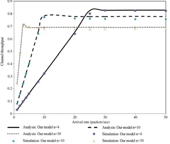
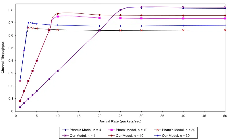
In order to verify our proposed analytical model, we compare theoretical analysis discussed earlier to the simulation results in Figure 2. This figure illustrates that the simulation results agree well with analytical results.

[image:8.595.308.539.96.181.2]

In Figure 3 we observe the impact of packet arrival rate on channel throughput as number of STAs varies. It is clear that for a given number of STAs in the net-work, increase in the packet arrival rate increases the channel throughput linearly in both models as long as the packet arrival rate is less than packet processing rate. However, as the channel throughput reaches its maximum, further increase in packet arrival rate makes channel throughput to saturate. This is because all STAs have a packet to transmit at any given slot. That is, packet arrival rate is more than the packet process-ing rate, which causes the saturation of throughput. It is observed that proposed model shows increase in throughput with an improvement of 1 to 4% compared to Pham’s model [14] with increase in number of STAs (n) from 4 to 30. This improvement is due to the checking of channel status in our proposed model be-fore decrementing the backoff counter value according to [1], which in turn decreases the probability of colli- sions and hence increases the probability of successful transmissions. This is also confirmed in Figure 5. However, at low packet arrival rate, performance of the proposed model is similar to Pham’s model. This is

Table 2. Summary of IEEE 802.11 DCF parameters.

Payload (PL) 8000 bits Channel bit rate 1 Mbps

Headers 576bits Prop. Delay 2µs ACK 320bits Slot Time 20µs

DIFS 50µs SIFS 10µs

Ql (Queue length) 50

because the number of competing STAs is small and also the packet arrival rate is less, and hence channel status may be idle for most of the time. We also find that maximum throughput value gets shifted to a lower value with increase in number of STAs. This is obvious as the number of competing STAs increases, probabil-ity of packet collisions increases consequently.

Figure 4 shows the variation of channel throughput with number of STAs for a given packet arrival rate. We observe that increasing the number of STAs in-creases the channel throughput linearly till a maximum value is reached in both the models. However, further increase in number of STAs after the throughput reaches a maximum value; we observe that the throughput decreases. This is because of the fact that increase in number of STAs increases packet collisions and hence reduction in throughput. It is observed that the proposed model shows increase in throughput with an improvement of 2 to 4% compared to Pham’s model with increase in number of STAs (n) from 8 to 50 for a fixed packet arrival rate of 15 packets/sec. This im-

Throughput vs. Packet arrival rate

0 0.1 0.2 0.3 0.4 0.5 0.6 0.7 0.8

0 5 10 15 20 25 30 35 40 45 50

Arrival Rate (packets/sec)

C

ha

n

ne

l Th

roug

hpu

t

[image:8.595.99.496.463.706.2]

Pham's Model, n = 4 Pham' Model, n = 10 Pham's Model, n = 30 Our Model, n = 4 Our Model, n = 10 Our Model, n = 30

[image:9.595.85.502.98.322.2]

Figure 4. Channel throughput vs. number of STAs with varying packet arrival rate.

ma er

valu

b-vio are m ing STAs

(hence robabi packet a

higher packet arriva

Fro re 5 we e that y of

collisi reases w rease in er of STAs in both th els. Due t cking of el statu n

STA befor lue, prob-

provement in throughput is again due to the checking of channel status before decrementing the backoff counter value by an STA. However, at low packet ar-rival rate and with less number of STAs present in the network, performance of the proposed model is similar to Pham’s model. This is because of the reason that the number of competing STAs is small and also the packet arrival rate is less, and hence channel status may be idle for most of the time. We also find that

ximum throughput value gets shifted to a high e with increase in packet arrival rate. This is o us as there small nu ber of compet

less p lity of

l rate. collisions) with

m Figu observ probabilit packet

ons inc

e mod ith inco che numbchann s by a e decrementing its backoff counter va

Probability of collision

0 0.1 0.2 0.3 0.4 0.5 0.6

0 5 10 15 20

Arrival r

P

ro

b

a

b

ility

o

f

c

o

ll

is

io

n

s

s v

2 ate (

s. Packet arrival rate

5 30 35 40 45 50

packets/sec)

Pham's Model, n = 4 Pham's Model, n = 10 Pham's Model, n = 30 Our Model, n = 4 Our Model, n = 10 Our Model, n = 30

et arrival rate with varying number of STAs. Figure 5. Probability of packet collisions vs. pack

Throughput vs .

0 0.1 0.2 0.3 0.4 0.5 0.6 0.7 0.8

0 5 10 15 20

Num

C

ha

nne

l Th

ro

ug

hpu

t

Num be r of STAs

25 30 35 40 45 50

ber of STAs

Pham's Model, λ = 5 Pham's Model, λ = 15 Our Model, λ = 5 Our Model, λ = 15

Throughput vs. Number of STAs

Pham’s Model, λ=5

[image:9.595.93.503.480.706.2]

ability of collision is small in the proposed model com-pared to Pham’s model. Due to this we observe higher throughput with our model compared to Pham’s model (Figures 3 and 4). Further, we find that probability of packet collision increases slowly for smaller packet arrival rate and then remains almost constant in both the models.

3. Performance Analysis under Slow

Rayleigh Fading Channel

The Markov model developed for perfect channel case (Figure 1) can be easily extended to capture the behavior of IEEE 802.11 DCF under slow Rayleigh fading chan-nels. However, there are certain differences that must be taken into account. Under the perfect channel assumption, the packet is not received successfully by an STA only when it is destroyed by collision. In a wireless environ-ment, signal between mobile STAs undergoes deep fades [16] due to movement of STAs. The radio link between moving STAs is termed as Rayleigh channel. The signal fades result in packet drops due to low signal-to-noise ratio (SNR). In [14], channel “uptime” and “down time” are defined as two states of the channel. Channel “up-time” is defined as the duration when the received signal power is above a given threshold. Channel “downtime” is defined as the du

is below a given th

two-state Markov model. Readers are reques

[14] for a detailed discussion on Markov model for Rayleigh channels.

However, under the Rayleigh fading channel assump-tion, packets can be dropped if there is a collision or the channel is “down”. Therefore, probability of packet not being received successfully (p) must take into account

the above-mentioned causes. By taking this into consid-eration, it is possible to use the Markov model (Figure 1) to analyze the performance of IEEE 802.11 DCF under the Rayleigh fading channel also.

Under the Rayleigh channel assumption, a packet can be destroyed either by collision or when the channel is “down”, that is,

(29) where

ration when the received signal power reshold. This can be modeled using a

1 0

1

) 1 (

1_{ }  _{  }

 n n

p   

2

0 1 e 

 _{ } 

ility of channe

which represents the steady state probab l being “down” and  represents the ratio between the power threshold and the root mean square (rms) value of received power. We can rewrite (29) and obtain transmission probability as,

) 1 /( 1

0

1 1 1



     

   

n p  

ted to refer

(30) Using (24) and (30), we can easily obtain p and hence τ

for a slow Rayleigh fading channel.

Having obtained the values of τ and p for a Rayleigh channel, the results in Section 2, (i.e., Equations (27) and (28)) can still be applied for the performance analysis of DCF. Next, we present the variation of channel through-put with varying packet arrival rate for a slow ayleigh

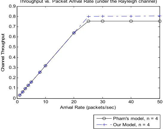
roughput increases ith increase in packet arrival rate before reach-ing a maximum value and then saturates even under Rayleigh fading channel. This is because the packet ar-rival rate is more than the packet processing rate of the system. As expected, saturation throughput decreases further under Rayleigh fading channel conditions as compared to a perfect channel assumption.

R fading channel.

From Figure 6 it is evident that th linearly w

0 10 20 30 40 50 0

0.1 0.2 0.3 0.4 0.5 0.6 0.7 0.8 0.9

Arrival Rate (packets/sec)

C

hannel

T

hr

oughput

Throughput vs. Packet Arrival Rate (under the Rayleigh channel)

[image:10.595.161.434.488.704.2]

Pham's model, n = 4 Our Model, n = 4

Figure 6. Channel throughput h varying packet arrival rate.

02.11 DCF do not comply with the 802.11 standard. In this paper, we have proposed an improved analytical model for DCF under finite load by closely following the specifications in 802.11 standard. Our analysis shown that our Markov model gives better insight into the op-eration of DCF in terms of channel throughput with varying packet arrival rate and number of STAs in a network under perfect and slow Rayleigh fading chan-nels compared with Pham’s model. Though we have shown our analysis for basic access mechanism of DCF, it is easy to extend our analysis for RTS/CTS-based ac-cess mechanism as well.

5. Acknowledgments

The first author expresses his sincere thanks to Prof. S.C. Laroiya, Director, National Institute of Technical Teach-ers’ Training and Research, Chandigarh, India for his constant support and encouragement. We express our sincere thanks to anonymous reviewers for their valuable comments which improved the quality of the paper.

1 AC, Vol. model for finite load IEEE 802.11 random access MAC,” Proceedings of ICC

of Networks, Vol. 2, No. 4, pp. 14-19, August 2007. [6] T.-S. Ho and K.-C. Chen, “Performance analysis of IEEE

802.11 CSMA/CA medium access control protocol,” Proceedings of 7th IEEE International Symposium on PIMRC 1996, Vol. 2, pp. 407-411, October 15-18, 1996. [7] H. S. Chhaya and S. Gupta, “Performance modeling of

asynchronous data transfer methods of IEEE 802.11 MAC protocol,” Wireless Networks, Vol. 3, pp. 217-234, August 1997.

[8] B. P. Crow, “Performance evaluation of the IEEE 802.11 wireless local area networking protocol,” Master’s thesis, Department of Electrical and Computer Engineering, University of Arizona, Tucson, AZ, 1996.

[9] R. K. Challa, S. Chakrabarti, and D. Datta, “A modified backoff algorithm for IEEE 802.11 DCF based MAC protocol in a mobile ad hoc network,” Proceedings of IEEE TENCON 2004, Vol. B. 2, pp. 664-667, November 21-24, 2004.

[10] Z. H. Fu, P. Zerfos, K. X. Xu, H. Y. Luo, S. W. Lu, L. X. Zhang, and M. Gerla, “On TCP performance in multihop wireless networks,” UCLA, WiNG Technical Report, 2002.

[11] F. Daneshgaran, M. Laddomada, F. Mesiti, and M. Mondin, “Unsaturated throughput analysis f IEEE ission channel , Vol. 7, No. 4, pp. 1276-1286, 2008.

E ACM Transactions on

bile Networks and Applications, Vol. 10, No. 5, pp. 691-703, 2005.

[15] L. Kleinrock, “Queueing systems,” Wiley, New S. Rappapor

4. Conclusions

Markov Models proposed in the literature for IEEE

IEEE 802.11 DCF for transient state conditions,” Journal

8

6. References

[1] “Part 11: Wireless LAN medium access control (MAC) and physical layer (PHY) specifications,” IEEE Standard, 2007 Edition.

2] G. Bianchi, “Performance Analysis of the IEEE 802.1 [

Distributed Coordination Function,” IEEE J-S 18, No. 3, pp. 535-547, March 2000.

[3] O. Tickoo and B. Sikdar, “A queue

2004, Vol. 1, pp. 175-179, June 20-24, 2004.

[4] Y. S. Liaw, A. Dadej, and A. Jayasuriya, “Performance analysis of IEEE 802.11 DCF under limited load,” Pro-ceedings of IEEE 2005 Asia-Pacific Conference on Communications, Perth, Western Australia, pp. 759- 763, October 3-5, 2005.

[5] R. K. Challa, S. Chakrabarti, and D. Datta, “Modeling of

and capture effects,” IEEE Transactions on Wireless Communications

o 802.11 in the presence of non ideal transm

[12] F. Daneshgaran, M. Laddomada, F. Mesiti, and M. Mondin, “A model of the IEEE 802.11 DCF in the pres-ence of non ideal transmission channel and capture ef-fects,” Proceedings of IEEE GLOBECOM’07, pp. 5112-5116, November 26-30, 2007.

[13] D. Malone, K. Duffy, and D. J. Leith, “Modeling the 802.11 distributed coordination function in non-saturated heterogeneous conditions,” IEE

Networking, Vol. 15, No. 1, pp. 159-172, February 2007. [14] P. P. Pham, “Comprehensive analysis of the IEEE

802.11,” Mo

York, 1975. [16] T. t, “Wireless communication: Principles