Considerations on Applying Cross Entropy Methods to the Vehicle Routing Problem

Received Jun 15, 2015 / Accepted Dec 17, 2015

Editorial Académica Dragón Azteca (EDITADA.ORG)

Considerations on Applying Cross Entropy Methods to the Vehicle

Routing Problem

Marta Cabo, Edgar Possani

ITAM, Department of Mathematics,

Río Hondo No.1, D.F. 01080, México City, México.

[email protected], [email protected]

Abstract: The cross entropy method was initially developed to estimate rare event probabilities through simulation, and has been adapted successfully to solve combinatorial optimization problems. In this paper we aim to explore the viability of using cross entropy methods for the vehicle routing problem. Published implementations to this problem have only considered a naive route-splitting scheme over a very limited set of instances. In addition of presenting a better route-splitting algorithm we designed a cluster-first/route-second approach. We provide computational results to evaluate these approaches, and discuss its advantages and drawbacks. The innovative method, developed in this paper, to generate clusters may be applied in other settings. We also suggest improvements to the convergence of the general cross entropy method.

Keywords: Cross Entropy Method, Heuristics, Vehicle Routing Problem.

1 Introduction

The vehicle routing problem (VRP) is a NP-hard combinatorial optimization problem. The problem is defined over a weighted graph G = (V, A), where V = {v0, v1, …, vn } is a set of nodes, and A = {(vi, vj) | i ≠ j, vi, vj∈V} the set of arcs. The weight of each arc (vi, vj) denoted by cij represents the travel cost of visiting nodes vj after vi. In this paper we consider symmetrical costs (cij = cji). A vehicle must visit each node (representing a client) once to satisfy its known demand di. The vehicle capacity is limited to Q (where di ≤ Q). The vehicle starts from the depot node v0, and if the sum of the demands of the clients exceeds that of the vehicle then, we need to perform several trips back and forth from the depot. There is an extensive literature on this classical version of the VRP, as well as a myriad of other versions that include additional characteristics; we refer the interested reader to [1]. The travelling salesman problem (TSP) may be considered a particular case where the capacity restriction does not come into play (i.e. Q = ), and we want to find a least cost tour that visits each client once starting and returning to the depot. However in contrast to the TSP, where instances involving thousands of clients may be solved by branch-and-cut algorithms, the most advanced exact algorithms for the VRP can only solve difficult instances of up to about 100.

The combinatorial nature and complexity of the problem have stimulated major developments in the fields of exact and heuristic algorithms. Recently, there has been special interest in developing metaheuristic to tackle combinatorial optimization proble ms where the search of the solution space is based on strategies that are able to extract knowledge during the search process. Throughout the search, such metaheuristic constantly evaluates the solutions obtained with the aim of extracting useful information to improve the future search. One such innovative metaheuristic is the cross entropy method (CEM) proposed by Rubinstein and Kroese [2], [3].

The cross entropy method (CEM) derives its name from the cross-entropy (or Kullback-Leiber) distance and was motivated by an adaptive algorithm for estimating probabilities of rare events in complex stochastic networks which involves variance minimization. It was soon realized that a simple modification of the CEM could be used to solve difficult combinatorial optimization problems. This is done by translating the original deterministic optimization problem into a related stochastic estimation problem, and then applying the rare event simulation machinery.

23

The only reference, we know of, that applies CEM to solve a version of VRP is by Chepuri and Homem-de-Mello [9]. Their problem specification assumes that the demand of a given customer is a random variable with known distribution, but the actual demand is known until the vehicle arrives at the customer. The vehicle runs out of stock before serving all customers. Thus, it returns to the depot and a penalty is computed for unvisited customers. Their objective is to minimize the expected cost calculated as the sum of all distances travelled, including the distance to the customer where the stock ran out and back to the depot, plus the penalties for the unvisited customers. They use CEM to solve a TSP over all customers using the approach suggested by De Boer, Kroese, et. al. in [3].

In this paper we discuss various implementations based on CEM for the VRP. First of all we evaluate the route-splitting approach by presenting results on two splitting methods. One proposed by Rubinstein and Kroese [2] that follows the basic criterion of returning to the depot when it is not possible to serve the next customer in the route. The second one solves a dynamic program to find the best feasible route, similar to the one developed by Prins et. al. [10]. Then we introduce a new cluster-first/route-second approach where CEM is used to find the best feasible cluster. This is the first time CEM is applied to clusterization, and we believe it could be extended easily to other combinatorial optimization problems involving the grouping of customers, tasks, or data.

The paper is organized as follows: in Section 2, we briefly describe the cross entropy method, and its application to the TSP. At the end of this section we also suggest improvements to the general CEM. A heuristic that constructs solutions for the VRP based on those obtained for the TSP using the CEM is explained in Section 3. A detailed description of our cluster-first/route-second heuristics is described in Section 4. Finally, in Section 5, we do a parameter analysis, and later compare the results obtained with the heuristics developed in this paper. We conclude by discussing the advantages and drawbacks of using CEM for the VRP and suggest further research areas to extent this work in Section 6

2 Cross Entropy Methodology

Cross entropy can be thought of as a model based search algorithm [11] where candidate solutions are generated using a parameterized probabilistic model that is updated using the previously seen solutions in such a way that the search will concentrate in the regions containing high quality solutions. The term model is used here to denote an adaptive stochastic mechanism for generating candidate solutions, and not an approximate description of the environment.

When using cross entropy to solve discrete optimization problems, one transforms the original problem into a rare event estimation problem, where monte-carlo simulation and importance sampling can be applied. In general we can think of the optimization problem as one of searching for a solution X*, that minimizes S, the objective function, over all X ∈ Ω (where Ω is the solution space). We want to find 𝛾∗

such that

min𝑋∈Ω𝑆(𝑋) = 𝛾∗= 𝑆(𝑋∗) .

We first change the optimization problem into a meaningful estimation problem. To this end we define a collection of indicator functions {𝐼{𝑆(𝑋)≤𝛾}} on Ω for various levels of 𝛾 ∈ ℝ. We also define a family of discrete probability densities

parameterized by a real-valued parameter (vector) P, and for a certain we have the associated stochastic estimation problem:

That is, the problem of estimating the expected probability of S(X) being less or equal than 𝛾 under parameter . Since 𝑆(𝑋) ≤ 𝛾

is a rare event when 𝛾 is close to 𝛾∗

, we can then apply the methodology of importance sampling and simulation to iteratively approximate f(X; P) through a parameter P* that allows 𝛾 to converge to 𝛾∗_{, and so this problem is equivalent to the optimization}

problem.

To estimate P* at each iteration a sample of N possible solutions X1, …, XN is generated, and via cross entropy P

*

24

𝑃∗_{= arg min} 𝑃

1

𝑁∑ 𝐼{𝑆(𝑋𝑖)≤𝛾}ln 𝑓(𝑋𝑖; 𝑃)

𝑁

𝑖=1

(1)

For more details on the general methodology, the reader is referred to [2] and [3]. We will explain in more detail the CEM implementation for TSP in the following subsection.

2.1 CEM for the TSP

A solution X = (x1, …, xn) for the TSP can be viewed as a vector where the i-th component represents the city visited in the i-th place on the tour. Notice that arc (i, j) belongs to tour X if for some k (k = 1, …, n – 1) xk= i and xk+1 = j, we will denote this as (i, j) ∈X. The goal of cross entropy is to minimize S(X), where S is the total distance travelled in tour X. S(X) = ∑𝑛−1𝑖=1 𝑐𝑥_𝑖,𝑥_𝑖+1+

𝑐𝑥𝑛,𝑥1 where ci,j is the distance from city i to city j.

We need to specify a mechanism for generating feasible random tours. To do so it is common to use a probability matrix P = (pij), where pij is the probability of visiting city j immediately after city i. There are several algorithms to generate a sample of tours X1,…, XN based on P, some can be found in [2], however in this this paper we use one found in [12] with complexity

O(n2). At this point it is important to note that P is the parameter to be estimated at each iteration of the cross entropy algorithm. It has been shown that P* (solution to (1)) for this particular problem is given by:

(2)

Note that with this estimation of P* we are taking into account those tours from the sample that have a good {𝐼_{{𝑆(𝑋)≤𝛾}}}, and counting the number of times arc (i, j) belongs to those tours. The next iteration of the algorithm will use this updated P* as the new P, until a convergence criterion is met. Thus the general cross entropy algorithm for the TSP can be summarized as:

Cross Entropy Algorithm for TSP (CE-TSP)

Step 1: Initialize α ∈ (0, 1) a smoothing parameter; t = 1 an iteration counter, and (1 – ρ) the quantile of the best performance of the sample to be taken into account for the estimation. Initialize Pt with pij=

1

𝑛−1 for i ≠ j, and pii=0, the initial uninformative

probability matrix to generate tours.

Step 2: Generate a sample X1, . . ., XN of N feasible tours for the TSP, using Pt as in [12]. Calculate the performances S(Xk) for k = 1, . . . , N, and order them in decreasing order so that S(X(1)) ≥ S(X(2)) ≥ ... ≥ S(X(N)). Let γt be the sample (1 – ρ) quantile of best

performances where γt = S(X(⌈(1−ρ)N⌉)).

Step 3: Use sample X(⌈(1−ρ)N⌉) , . . . , X(N) to calculate Pt+1 = (pij) as

Step 4: Update Pt+1 = αPt + (1 − α) Pt+1

Step 5: For some t ≥ d, in our case d = 5 if:

γt = γt−1 = γt−2 = … = γt−d,

stop the algorithm, otherwise t = t + 1 and go to step 2.

In step 4, to smooth the convergence at each iteration t + 1, transition matrix Pt+1 also considers the information of the previous

iteration, Pt, so that we update Pt+1 = α Pt + (1 − α) Pt+1, where α ∈ (0, 1) is the smoothing parameter. Decisions on the value of

parameters N, ρ and α impact on the quality of the final solution, and will be discussed in subsection 5.1.

For the most commonly used version of the CE method the optimal solution is given by γt at the last iteration. Although we keep

25 2.2 Improvements on convergence of CEM

We have observed that in some special cases at each iteration γt is not a strictly decreasing function. This happens when the

optimal and close to optimal solutions are very rare, and most solutions are far from the optimal. Let us illustrate this by considering a 10-city TSP where ci,i+1 = 1, ∀i = 1, . . . , 9; and cij∈ [2,10], when | i − j | ≥ 2, ∀i, j = 1,...,10. In this case the optimal tour has a cost of 10 (with probability of occurrence of 1/10!) and S(X(⌈(1−ρ)N⌉)) ≥ 14 in all samples with a very high

probability. Furthermore γt oscillates between different values slowing down the convergence.

To improve the convergence in such cases we propose, instead of using the ρN best performances at each iteration, to take only those that improve the last best performances to update Pt. If there are none, then take the last Pt−1 to do the update, ignoring the

current sample. This is an improvement on the standard version of CE that allows a better convergence for the special cases where γt does not decrease at each iteration. Hence, substituting Step 3 of the standard algorithm by the following:

Step 3 (modified): Let γt∗ be the value of the best γt observed so far in the algorithm. Then if S(X⌈(1−ρ)N⌉) ≤ γt∗ use sample

X(⌈(1−ρ)N⌉),…,X(N) to calculate Pt+1 = (pij)


otherwise we may encounter two cases

a) S(X⌈(1−ρ)N⌉) > γt∗ and S(X(N)) ≤ γt∗. Find j′ such that

j′ = min 𝑗∈{(1−𝜌)𝑁,…,𝑁}{𝑗 | 𝑆(𝑋(𝑗)) ≤ 𝛾𝑡∗}

and calculate Pt+1 = (pij) as

b) S(X⌈(1−ρ)N⌉) > γt∗ and S(X(N)) > γt∗ keep Pt+1 = Pt.

Note that with this modification in fact we allow a variable sample size to update Pt. This modification has never been proposed in the literature.

3 CEM for Route Splitting

General vehicle routing heuristics can be divided into two types: route splitting, and cluster-first/route-second methods. Route splitting first creates a big tour including all customers in the system, and then splits the tour into feasible routes. The feasibility of a route is determined by the vehicle capacity and may consider total distance travelled, maximum number of customers, or time windows constraints. In this paper we only consider the capacity constraint, but others can be easily included in our implementation.

In this section we study two splitting methods, which help construct solutions to the VRP. CEM is first used to solve a TSP, as explained in 2.1 and 2.2, which visits all customers, ignoring the capacity constraint. Based on that solution, we then apply either a sequential splitting or a dynamic programming splitting to compute the travel costs and update the probability matrix that generates the tours in the sample.

3.1 Sequential Splitting

26

than this capacity, then the vehicle returns to the depot from the current customer, and the next route is generated starting in the last unserved customer. Hence, the cost of this solution S(X) is the sum of all the route costs.

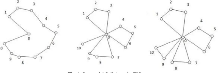
This splitting method does not consider all feasible VRP routes. For example, as illustrated in Figure 1, on an instance with 10 customers (n = 10) where the demand of each customer is dj= 10, and vehicle capacity Q = 30, this algorithm will always create four routes: the first three with three customers and the last one serving only one (as shown in the middle graph of Figure 1 ). However the algorithm excludes solutions where two routes serves 3 customer and two other serving two (as shown in the right hand graph of Figure 1). Hence, there are feasible routes that are never going to be considered by this algorithm.

Fig. 1. Sequential Splitting of a TSP tour

To avoid this, we propose a dynamic programming splitting procedure that not only explores all feasible splitting but actually for a given TSP-tour gives the optimal VRP routes, as explained in the next subsection.

3.2 Dynamic Programming Splitting

To obtain the best VRP routes for a given sequence of customers, the decision problem is transformed into a shortest path problem, to later apply a polynomial-time dynamic program to solve it. Given a sequence of customers to visit x1, x2, … , xn we construct a graph that contains n + 1 nodes where node 0 stands for the depot, and node i for customer xi. An arc (i, j) in the graph indicates that route x0 − xi+1 − xi+2 − … − xj− x0 belongs to the VRP solution. We are interested in minimizing the total

traveling cost of all routes, hence the cost of arc (i, j) can be calculated as T(i, j) = 𝑐𝑥0,𝑥𝑖+1+ ∑ 𝑐𝑥𝑘,𝑥𝑘+1

𝑗−1

𝑘=𝑖+1 + 𝑐𝑥_𝑗,𝑥0. The vehicle capacity constraint requires L(i, j) =∑ 𝑑𝑗

𝑗

𝑘=𝑖+1 ≤ 𝑄, so that we should only consider arcs (i, j) that comply with this restriction as

pointed out by [10], alternatively we can think of T(i, j) = ∞ for such cases. A path that joins node 0 with node n indicates a feasible splitting of customers into routes. Hence finding the shortest path between node 0 and node n is equivalent to finding the best VRP solution.

Let Fk(j) the shortest path from node 0 to node j that uses no more than k arcs. Initialize Fk(j) = ∞, if j ≠ 0 and Fk(0) = 0 ∀k = 1, …, n. Then the dynamic programming recursion for k = 1,… , n is:

Fk(j) = min{i| i<k, L(i, j) ≤ Q} {T(i, j) + Fk−1(i)}, j = k, …, n

Where the shortest path length is given by Fn(n) and the VRP solution can be obtained by backtracking from node n at stage n. Hence, for any given sequence X = (x1, …, xn) its least cost is S(X) = Fn(n) when using the dynamic programming splitting procedure.

It is easy to see that to include other costs to the objective function, one only needs to add them to T(i, j); and to include restrictions like time windows or maximum distance travelled, omit the arcs (i, j) that not comply with these restrictions.

4 CEM for Clustering

27

(randomly) selected as a seed for the next cluster, and the same technique applied to completing it, continuing in the same manner until all customers are assigned to the different clusters.

Unlike previous simple methods, we consider the decision of assigning customers to clusters via a probability distribution to be estimated through cross entropy. The probability distribution will ultimately store the information on which customer-cluster assignment yields the best solutions. To evaluate the objective function for each assignment, a TSP is solved within each cluster and all distances travelled are added. Cross entropy uses the best assignments found to update the probability distribution iteratively. As far as the authors know, this is the first application of CEM for clustering.

When assigning customers to clusters the total demand of the customer within a cluster should not violate the capacity restriction of the vehicle. To ease the creation of such feasible clusters we allocate customers to clusters in non-increasing order with respect to their demand. This ensures that those customers with bigger demand are assigned first in the clustering process, when the cluster capacity is bigger. Let Y = (y1, …,yn) be a vector where yi = k means that customer i belongs to cluster k. Consider a probability matrix A = (aik) of n × K where aik represents the probability of customer i belonging to cluster k, initially aik = 1/K. K is calculated as

𝐾 = ⌈∑ 𝑑𝑖

𝑛 𝑖=1

𝑄 ⌉

The algorithm for generating random feasible clusters can be described as follows:

Cluster Generation Algorithm (CGA)

Step 1: Let C(k) be the remaining capacity of cluster k (k = 1, …, K). Initialize C(k) = Q∀k. Initalize i = 1 to be the first customer to be assigned.

Step 2: Generate an observation k′ from probability distribution P(yi = k) = aik, where aik is the probability of customer i belonging to cluster k. Assign customer i to cluster k′, that is, set yi = k′. Calculate the remaining capacity of cluster k′ as

C(k′) = C(k′) − di, and let aik = 0 ∀k ≠ k′ and aik′ = 1.


Step 3: Adjust the probability matrix given the new capacity of cluster k′ so that for every row in A: r = i + 1, …, n where C(k′) < dr:

3.1) Set ark′ = 0


3.2) Let norm = ∑𝐾𝑘=1𝑎𝑟𝑘 and for k = 1, …, K:

ark = ark/norm

Step 4: Let i = i + 1. If i ≤ n go to Step 2.

At the end of this process A will have the information of which customer belongs to each cluster (those aik = 1). Note that Step 3 only adjusts those probabilities corresponding to an infeasible assignment of a customer to a cluster when the customer’s demand is bigger than the capacity of cluster k′, and norm is a normalization factor so that the sum of probabilities of a customer r being assigned to all feasible clusters equals one.

To solve the TSP for each cluster we have tried two algorithms. One is the CE-TSP algorithm explained in section 2.1. The second one is a multi-start greedy heuristic, where the first customer in the route can be any in that cluster, and once this customer is visited we continue to the nearest one until all are visited and return to the depot. The best of all these routes is chosen as the TSP solution for that cluster. Independent of which heuristic is used, S(Y) denotes the total cost of that VRP solution. This is obtained as the sum of the travel costs of the K tours, calculated by the chosen heuristic, under cluster assignment Y. Hence, to apply CEM to the problem, we need to generate a sample of N’ feasible clusters: Y1, …, YN’, order them in decreasing order of S(Yj) and use the ρ best performances to update cluster assignation probability matrix A as:

Similar to the implementation of CEM for the TSP, this calculates the number of times customer i is assigned to cluster k over the sample size considered. As before, At, the cluster assignation probability matrix at iteration t, is updated with a smoothing parameter α′:

28

There are different parameters to be set on the CEM algorithm; we evaluate the impact these have on the performance of the algorithm in the following section.

5 Evaluation of CEM for VRP

In this section we start by evaluating the impact of different parameters have on the algorithm. Later, we present results of the application of cross entropy using route splitting methods, and then with cluster-first/route-second methods. We conclude this section by comparing the best results of both approaches.

N: Size of the sample. The bigger the size, the more elements we generate under a given probability matrix. We need to read and temporarily modify the matrix as many times as the size of each element in the sample. Likewise, for a fixed ρ, as N increases, the ρN quantile considers more elements to update the probability matrix. Hence, at iteration t we need to generate and evaluate more observations, thus increasing the number of operations to be performed.

A small sample size might not have enough information to adequately update the matrix. On the other hand a bigger sample size does not necessarily yield better elements. It is important to notice, that the probability matrix may not have the best information at the first iterations. There is a trade off between size of the sample, number of operations (time) and quality of the information.

ρ: Quantile to be considered for the best performances. This denotes the proportion of elements in the sample taken as best performances to update the matrix. Initial experiments showed, that for a given problem size, the important factor was Nρ, the number of elements taken for the update. This size can either be obtained by modifying ρ or modifying N. We do not modify ρ for different sample sizes, but adjust N to always take the same number of elements for the best performances. Throughout our experiments ρ = 0.05 is used, always considering the 5% best performances.

α: Smoothing parameter to update probability matrix. If α = 0 only the information on the current iteration is used to generate the new probability matrix. As α approaches 1, the information of the previous iteration becomes more important. High values of α implies little changes on the probability matrix from one iteration to the other, this tends to slow down the convergence but might allow for a more thorough exploration of the solution space.

Previous evaluations [13] have shown that to solve the TSP via cross entropy N = 10n2, where n is the number of customers to visit, and α = 0.7 yields good results for n < 50. For n ≥ 50 it was shown that N = n2 is a good sample size. We have kept these parameter settings when solving the VRP instances with the route splitting methods.

Recall that for the cluster-first/route-second scheme, as CEM may be applied both for clustering and for solving the TSP of each route, the sample size has to be set twice: once for the clustering N′, and then when applying CEM to find the best order in which to visit the customers within each cluster, N. We have kept N = 10n2, and α = 0.7, as clusters always have less than 50 customers. However, as this is a new design for CEM there is a need to find the best N′ and α′.

We have done an evaluation on the impact the above parameters have on the performance of the algorithm. We ran the instances on a Mac OS X Lion 10.7.4 with a Intel Core i7 2.8 GHz processor and 4 GB of RAM. Our implementation is not specially optimized and running times could be improved. As an example, in Figure 2, we show results for an instance with 31 customers and 5 vehicles (B31-k5 found in the benchmarks of [14]). We have plotted the variation on the average performance 𝛾̅𝑡 (on the

left hand vertical axis, and solid lines) and the variation on the average time (on the right hand vertical axis, dash lines) for different sample sizes N′ = 150, 250, 350, 450 and varying smoothing parameters α′ = 0.1, 0.3, 0.5, 0.7, and 0.9.

29

N′ = 450 about 810,000 TSP samples of approximately 6 customers per iteration. There is considerable improvement in quality solution from a size N′ =150 to N′ =250, and marginal for N′ = 350 or 450, with a dramatic increase in computation time (up to 4 times). We believe from our experiments that a compromise of a good quality of solution with reasonable computational times is reached when using a sample of size N′ = 250.

Fig. 2. Average quality and time performance of the algorithm for varying N’ and α’

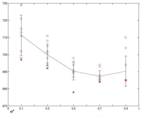
In Figure 3 we have plotted the performances for N′ = 250 and different values of α′ = 0.1, 0.3, 0.5, 0.7 and 0.9. We show the average performance in the solid line, its standard error interval, as well as the actual performances over the 10 runs for each specific α′ (small circles). It can be concluded form these results that the best average performance is obtained when α′ = 0.7 with the least variation for the different runs. However, note that for α′ = 0.5 we did manage to get a better result in one run. Throughout our experiments we have then set N′ = 250 and chosen the best result for either α′ = 0.7 or α′ = 0.5.

Fig. 3 Performance for N’ = 250 and different values of α’

When using the greedy heuristic to calculate the solution for the TSP’s with N′ = 150, 250, 350, 450 the results were worst in quality every time but the computing time was reduced drastically. Thus it seemed reasonable to increase the sample sizes, as better solutions are found on average with bigger sample sizes. When K increases so does the possible clusters a single customer might belong to, hence we have considered sample sizes that depend on K, N′ = 50K, 100K, 150K, 200K, 500K, 750K for different instances. In Figure 4 the graph shows the variation on the average performance 𝛾̅𝑡 (on the left hand vertical axis, and

30

Fig. 4 Average quality and time performance of the algorithm for varying N’ and α’

It can bee seen that when N′ = 500K the average time was under 5 seconds to find a solution for those α’s that yield the best results. As N′ increased to 750K the average time increases considerably. However the solution quality does not improve by more than 1%. We observed similar results for other instances. Thus we decided to choose N′ = 500K as the sample size for this implementation. Regarding the choice of α we saw that on average for the instances tried α = 0.3 gave the results with best average and least variation.

5.2 Results for Route Splitting Methods

Evaluations have been done over a set of 28 instances of various sizes (from 22 to 101 customers) and number of clusters (3 to 14 clusters), obtained from [14]. There are three classes of instances, class A, B and E. Class A uses a set of customers uniformly distributed in the plane, where as in class B customers are distributed in clusters. Class E is a mix of both, some customers are clustered together and some are distributed randomly over the plane.

31

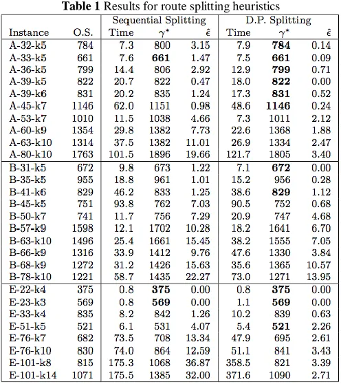
In Table 1 we summarize the results for sequential and dynamic programming (D.P.) splitting implementations. The first columns state the instance name and the optimal solution (O.S.), for each method we first show the average running time (in seconds) over 10 runs, the best solution obtained γ∗_{, and the average error 𝜖̂ as a percentage. This error 𝜖̂ is calculated as the}

average difference between the observed solution and the optimal solution over the optimal solution. Bold figures denote that the optimal was achieved by the algorithm.

As expected, D.P. splitting yields better results in all instances, hence improving the previously published results by [2] and [13]. The optimal solution was obtained in 11 out of 28 instances. The average error is no greater than 14%, and in 24 out of 28 it is less than 5%. It seems that the algorithm gives on average a better solution when customers are randomly distributed. On the other hand Sequential splitting only finds the optimal solution in 3 of the 28 instances, and in half the instances the average error is greater than 5% and as high as 36%, and although for some instances it runs faster, the solution is never better than the one obtained with D.P. splitting.

As the sample size increases so does the running time. This is not only due to the fact that as n increases the computation effort to generate a single element of the sample increases; the main impact comes from the fact that the sample size is a quadratic function of the number of customers. The cluster-first route-second implementation aims to reduce this running time by downsizing the sample-generating matrix from one of size n×n to one of size n×K, and instead of generating 10n2 samples generate 500K. This time reduction will be evident in the next section when running CEM for clustering and the modified greedy algorithm for the TSP, but not when using CEM to solve each TSP as explained in section 5.1.

5.3 Results for Cluster-first/Route-second Methods

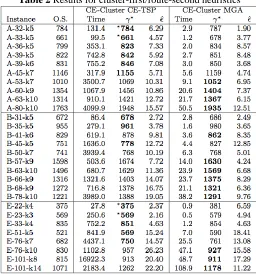
Evaluations have been replicated on the same data set as the one used in section 5.2. In Table 2 we summarize the results for the cluster-first route- second implementation. Columns under heading CE-Cluster CE-TSP shows results where CEM is applied both for clustering and routing, and CE-Cluster MGA shows those for CEM applied for clustering and the greedy heuristic for routing. In this table bold figures denote where each implementation finds the best result, and is preceded by ∗ when it reaches the optimal solution.

32

CE-Cluster MGA runs considerably faster than CE-Cluster CE-TSP. There are 5 instances where CE-Cluster CE-TSP takes more than 1 hour to converge, where as CE-Cluster MGA only has one instance that takes more than 1 minute (and less than 2). An extreme case is instance E-101-k8 where CE-Cluster CE-TSP runs on average for 4 hrs. 42 minutes and CE-Cluster MGA runs only in 48.7 seconds. The use of CEM to solve the TSP within each cluster is time consuming but we can see we only got optimal solutions when using this approach. This confirms that using CEM for routing is not as bad choice as one might think, however it is time-wise impractical.

The best solution over all runs was, in half of the instances, obtained with CE-Cluster CE-TSP. However CE-Cluster MGA solutions have less variability in 75% of the instances as observed in the results, this may be explained by the fact that CE-Cluster MGA always gives the same solution for a given set of customers. CE-CE-Cluster CE-TSP performs better in smaller instances, and CE-Cluster MGA on instances with more than 50 customers and more than 7 clusters.

Comparing the results of the clustering versus the splitting i mplementations, we focus on the winning heuristics: CE-Cluster MGA and D.P. Splitting. CE-Cluster MGA runs faster than D.P. Splitting in almost all instances. However, CE-Cluster MGA only found better solutions in two cases (B-63-k10, B-78-k10). Which proves that using CEM for clustering may be a good approach for solving the VRP if we improve the quality of the routing heuristic, provided the running time is not compromised.

6 Conclusions and further research

In this paper we have improved the quality and running times of previous implementations of CEM to VRP. We designed and explained how CEM can be adapted both for a route splitting and cluster-first route-second approach. We believe that an important contribution of this paper is the design of a new cross entropy algorithm to generate feasible clusters, the ideas of which may be adapted to other clustering problems.

In this paper we proposed and tried a modification of the general CEM to allow a variable sample size to update Pt. Another interesting modification is the “elite sample” version of the CE method [15], where the best performances over all iterations are always stored and used for the update of Pt. For the “elite sample”, as with the standard algorithm, the sample size is kept constant. It would be interesting to investigate if there is an advantage of keeping the best performance overall samples together with our variable sample size, and evaluate the effect of both modifications on the quality of the solutions and running time of the heuristic.

An extensive analysis of the parameter setting was done with its impact on the solution quality and time. From the results we can see that the best solution seems to get on average further apart from the optimal solution as the size of the VRP instances increases. However, we believe that this may be improved by adding to the first sample a set of initial solutions created via fast and reliable constructive heuristics. Thus, the transition matrix will initially consider this information when updating Pt and ideally converge to a better solution. In some sense this is guiding the search with additional information, not relying on the uninformative initial distribution alone. This seems a promising future venue of research.

Acknowledgements: The authors would like to thank Asociación Mexicana de Cultura A.C. for their support.

References

1. Toth, P., Vigo, D.: The Vehicle Routing Problem. SIAM monographs on discrete mathematics and applications (2002)


2. Rubinstien, R.Y., Kroese, D. P.: The Cross-Entropy Method: A unified approach to combinatorial optimization, monte-carlo simulation, and machine learning. Springer (2004)

3. De Boer, P.-T., Kroese, D. P., Mannor, S., Rubinstein, R.Y.: A Tutorial on the Cross-Entropy Method. Annals of Operations Research 134, 19-67 (2005)


4. Laguna, M., Duarte, A., Martí, R.: Hybridizing the cross-entropy method: An application to the max-cut problem. Computers & Operations Research 36, 487-498 (2009)

5. Caserta, M., Quiñonez Rico, E., Marquez Uribe, A.: A cross entropy algorithm for the Knapsack problem with setups. Computers & Operations Research 35, 241-252 (2008)

6. Caserta, M., Cabo Nodar, M.: A cross entropy based algorithm for reliability problems. Journal of Heuristics 14, 5, 479-501 (2009)
 7. Alon, G., Kroese, D. P., Raviv, T., Rubinstein, R. Y.: Application of the cross-entropy method to the buffer allocation problem in a

simulation-based environment. Annals of Operations Research 134, 137-151 (2005)

8. Bekker, J., Aldrich, C.: The cross-entropy method in multi-objective optimisation: An assessment. European Journal of Operational Research 211, 112-121 (2011)

33

10.Prins, C., Labadi, N., Reghioui, M.: Tour splitting for vehicle routing problems. International Journal of Production Research 47, 507-535 (2009)

11.Zlochin, M., Birattari, M., Meuleau, N., Dorigo, M.: Model-Based Search for Combinatorial Optimization: A Critical Survey. Annals of Operations Research 131, 373-395 (2004)

12.Vaisman, R.: TSP random tour generation algorithm CE Method. URL: http://iew3.technion.ac.il/CE/files/papers/TSP.pdf. Accessed May 2015.

13.Possani, E., Herrera Musi, C., Cabo Nodar, M.: An Evaluation of the Cross Entropy Method to Solve Vehicle Routing Problems. Proceedings of the Latin-American Operations Research Workshop, TLAIO IV, (2011). Available at SSRN: URL:

http://ssrn.com/abstract=1946382. Accessed May 2015.

14.VRP benchmark problems URL: http://www.bernabe.dorronsoro.es/vrp/ Accessed May 2015

15. Costa, A., Jones, O. D., Kroese, D. P.: Convergence properties of the cross-entropy methodfor discrete optimization.