DOI: 10.1051/0004-6361:20020760 c
ESO 2002
Astrophysics
&
Automatic observation rendering (AMORE)
?
I. On a synthetic stellar population’s colour-magnitude diagram
Y. K. Ng
1,2, E. Brogt
1,3, C. Chiosi
4, and G. Bertelli
2,51 TNO TPD Space, PO Box 155, 2600 AD Delft, The Netherlands
2 Padova Astronomical Observatory, Vicolo dell’Osservatorio 5, 35122 Padua, Italy 3 Kapteyn Astronomical Institute, PO Box 800, 9700 AV Groningen, The Netherlands 4 Padova Department of Astronomy, Vicolo dell’Osservatorio 2, 35122 Padua, Italy 5 National Council of Research, IAS, Rome Italy
Received 14 February 2002/Accepted 15 May 2002
Abstract.A new method,AMORE– based on a genetic algorithm optimizer, is presented for the automated study of colour-magnitude diagrams. The method combines several stellar population synthesis tools developed in the last decade by or in collaboration with the Padova group. Our method is able to recover, within the uncertainties, the parameters – distance, extinc-tion, age, metallicity, index of a power-law initial mass function and the index of an exponential star formation rate – from a reference synthetic stellar population. No a priori information is inserted to recover the parameters, which is done simultane-ously and not one at a time. Examples are given to demonstrate and to better understand biases in the results, if one of the input parameters is deliberately set fixed to a non-optimum value.
Key words.methods: data analysis, numerical – stars: HR-diagram, statistics
1. Introduction
The present data flow of many ongoing surveys – such as 2MASS (Beichman et al. 1998; Skrutskie 1999), DeNIS (Epchtein et al. 1997, 1999), EIS (Renzini & da Costa 1997; da Costa 1997; da Costa et al. 1998), OGLE-II (Udalski et al. 1997; Paczy´nski et al. 1999), SDSS (Fan 1999 and refer-ences cited therein), and even upcoming surveys as GAIA (Gilmore et al. 1998; Perryman et al. 2001) – is so large that one requires either a semi-automated or a fully automated method to analyse the colour-magnitude diagrams (CMDs) in the resulting databases. In this paper we discuss the develop-ment and the tests of an automated analysis method, which fully employs the colour and magnitude information available about the stars populating the CMD. Our method is based on an implementation of the CMD diagnostics suggested by Ng (1998). The method uses, in contrast to other techniques (see Bertelli et al. 1992; Gallart et al. 1996 & 1999; Geha et al. 1998 Harris & Zaritsky 2001; Hernandez et al. 1999;
Send offprint requests to: Y. K. Ng, e-mail:[email protected] ? Tables A1–A3 are only available in electronic form at
http://www.edpsciences.organd at the CDS via anonymous ftp tocdsarc.u-strasbg.fr (130.79.128.5)or via
http://cdsweb.u-strasbg.fr/cgi-bin/qcat?J/A+A/392/1129
Holtzman et al. 1997 & 1999) the full, unbinned distribution of magnitudes and colours of the stars populating the CMD.
The purpose of this paper is to verify that astrophysical parameters for a synthetic single stellar population can be reliably retrieved with the so-called “AutoMaticObservation
REnderer”AMORE. In Sect. 2 an outline ofAMOREis given together with its individual building blocks. In Sect. 3 we out-line the method we use and in Sect. 4 we describe the tests performed with synthetic stellar populations. The results are given in Sect. 5 and we discuss in Sect. 6 the practical limits on the convergence, which is imposed by some degeneracy of the parameter space. We end with prospects on forthcoming tests, recommendations for improvements, and an outlook on future developments.
2. AMORE
2.1. Project outline
AMOREtries to find the best matching synthetic CMD to an observed CMD. Such a synthetic CMD contains for stellar ag-gregates the contribution of one or more stellar populations at the same distance. In the case of a CMD along a particular line of sight in our Galaxy the synthetic CMD can moreover contain the contribution of various populations with stars distributed at different distances.
In this paper we focus on the implementation and the perfor-mance ofAMOREfor the fitting of CMDs. For sake of argu-ment only one, single stellar population has been considered. The implementation of automatic fitting CMDs with multiple stellar populations with stars at the same or different distances will be subject of forthcoming papers.
2.2. Building blocks
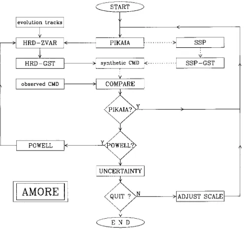
AMORE, see Fig. 1 and Sect. 3.1 for details, combines various analysis tools developed and improved at Padova during the last decade. Conceptually, it is made up out of the following building blocks:
– a synthetic Hertzsprung-Russell Diagram generator (here-after referred to asHRD-ZVAR see Sect. 2.3),
– a mockup version of the HRD Galactic Software Telescope (HRD-GST, see Sect. 2.4),
– a statistical diagnostic tool to compare the observed and synthetic CMDs with each other (Ng 1998), and
– thePIKAIA(extended version) andPOWELLoptimizers (see respectively Sects. 2.6 and 2.8), which search for the best fit between an observed and a synthetic CMD in a multi-parameter space.
In the following subsections a description is given of the vari-ous building blocks.
2.3.
HRD-ZVAR
In the late-eighties Bertelli developed a code to generate synthetic Hertzsprung-Russell diagrams (HRDs) from the isochrones computed by the Padova group (cf. Chiosi et al. 1989). Initially the synthetic colour-magnitude diagram (CMD) technique was applied mainly in the studies of LMC open clus-ters1(see for example Bertelli et al. 1985, 1990 or Chiosi et al. 1989), through which the amount of convective overshoot was calibrated for the computation of a new generation of stellar evolutionary tracks. Successive improvements were gradually applied when new sets of evolutionary tracks (see Bertelli et al. 1994 for details) were computed with improved radiative opac-ities (Iglesias et al. 1992).
The backbone of HRD-ZVAR, the extended version of the HRD generator, is formed by the evolutionary tracks computed by Bertelli et al. (1990; Z = 0.001), Bressan et al. (1993; Z = 0.020), and Fagotto et al. (1994a,b,c;Z = 0.0004, 0.004, 0.008, 0.050, 0.10). The metallicities of the tracks follow the enrichment law ∆Y/∆Z = 2.5 (see references cited in Chiosi 1996 and Pagel & Portinari 1998).
HRD-ZVAR indicates that the metallicity Z is not limited to the fixed values for which the evolutionary tracks have been computed, but is variable through interpolation between 1 The analysis technique with stellar ratios was employed. The rea-son for this is that ratios are less sensitive to uncertainties in certain regions in the CMD, which might not be reproduced properly due to various reasons such as the input physics used for the calculations of the stellar evolutionary tracks or the transformations from the theoret-ical to the observational plane.
the metal-poorest and metal-richest tracks available inside the database of evolutionary tracks. In this way one is able to gener-ate synthetic stellar populations with a smooth metallicity cov-erage. A prerequisite however is to use a complete and homo-geneous library of evolutionary tracks and some improvements are expected if one adopts a grid of tracks with a smoother metallicity coverage.
HRD-ZVAR has been distributed (privately) to various re-search groups and is also referred to asZVAR2. The version dis-tributed, modified, and used by for example Aparicio (1999), Gallart (1998), and Ng et al. (1996, 1997) is from now on re-ferred to as V1.0. Version V1.6 is used for the simulations and results presented in this paper. This version contains a number of modifications and improvements which speeds up the code and fixes some (rarely encountered) bugs which interfered with the automatic minimization process. Although various analy-sis methods are available, we limit ourselves here to the de-scription of the parameters related to theHRD-ZVARas adopted forAMORE.
After selection of a set of tracks with fixed metallicity and the choice of the parametersηRGB andηAGB, (the mass loss along the Red Giant Branch (RGB) and the Thermally Pulsing Asymptotic Giant Branch (TP-AGB) phases respectively), the major input to be specified forHRD-ZVARare:
– the metallicity range,Zranges fromZmintoZmax;
– the age range, the age ranges fromtmintotmax;
– the slopeαfor the power-law IMF (Initial Mass Function); and
– the indexβfor the exponential3SFR (Star Formation Rate). The luminosity and effective temperature for each synthetic star of arbitrary metallicity is transformed to an absolute magni-tude in a photometric passband with the method outlined by Bertelli et al. (1994) and Bressan et al. (1994). Default setup forHRD-ZVARis theU BVRI JHKLMN4broadband photomet-ric system. The setup can be altered to mimic any system, given the description of the spectral response of the filter and the de-tector of the photometric system.
2.4.
HRD-GST
HRD-ZVAR was integrated in a galactic model by Ng (1994, 1997ab). TheHRD-GST(Galactic Software Telescope) has been applied in the studies of the galactic structure towards the Galactic Centre (Ng et al. 1995, 1996 and Bertelli et al. 1995, 1996) and other regions in our Galaxy (Ng et al. 1997). In this paper we do not require the full complexity of the structural 2 Note that an older and modified version of HRD-ZVAR is actu-ally the program used to generate the Bertelli et al. (1994) isochrones. HRD-ZVARis free of the interpolation difficulties as reported by Olsen (1999).
3 The SFR is only fixed for the time being to the adopted exponen-tial shape.
Fig. 1.AMOREflowchart: schematic diagram of the individual build-ing blocks. PIKAIA outlines the direction of the evolution paths to be investigated. Input for the stellar population synthesis engine HRD-ZVARis the Padova library of evolutionary tracks. The luminosity and effective temperature for each synthetic star of arbitrary metallic-ity is then transformed to an absolute magnitude in a photometric pass-band with the method outlined by Bertelli et al. (1994) and Bressan et al. (1994). The synthetic HRD is then “observed” and “detected” through a Monte Carlo “observing run” with theHRD-GST. Note that an alternative route is possible with single stellar populations (SSPs). The synthetic CMD is compared with the observed diagram and a fit-ness parameter is subsequently communicated toPIKAIA, which sug-gests a new set of parameters for each trial. The iteration lasts for a user defined, fixed number of trials.POWELL’s method of minimization is subsequently applied to get closer to the local or global minimum. After computation of the uncertainties for each parameter the evolu-tionary run is either aborted or a newPIKAIA cycle is started after shrinking the limits of the parameter space (see Sect. 2.9).
properties from the GST model. We only use a limited num-ber of options to “observe” a synthetic HRD at the suggested distance and to simulate the photometric errors, extinction and crowding.
A table of the photometric errors, covering a specific mag-nitude interval per passband, is used and the program inter-polates linearly to obtain the intermediate values. We assume for the simulation that the photometric errors are Gaussian dis-tributed. A different description of the photometric errors will be used when published artificial star tests (Stetson & Harris 1988; Gallart et al. 1999) on an observational data set are in-dicative for a significant deviation from a Gaussian behaviour. The visual extinction is simulated with the average value pro-vided and appropriately scaled to a value in different pass-bands. In theUBVRIpassbands we adopted the scaling accord-ing to van de Hulst (1949; curve No. 15) and for theJHKLMN passbands we follow the scaling laws provided by Rieke & Lebofsky (1985). We do allow for some random scatter around the average extinction. However, we do not consider (yet) the effects due to patchiness of the extinction along the line of
sight. Ng & Bertelli (1996) demonstrated that this is in first ap-proximation, visually almost indistinguishable from a random scatter around an average extinction.
In many studies the observations are crowding limited, due to the increasing number of stars towards fainter magnitudes. Crowding gives rise to star blends which affects the magnitude and the colour of the stars. The group of stars will be detected as a single star with a magnitude equal to the sum of the stellar flux of the stars involved in the stellar blend. The remaining stars are “hidden” from detection.
The blends are well described as unresolved, apparent bina-ries. The simulation of apparent binaries is made with an iter-atively improved blending probability, which is defined as the probability that a star within a given ensemble of stars might blend with another star from the same population. Each syn-thetic star within a stellar population is tested against the blend-ing probability.
The percentage of artificial binaries is with this scheme about twice the blending factor. The blending factor in diff er-ent passbands is not necessarily the same and the occurrence of star blends is furthermore not necessarily correlated, due to possible differences in the exposure time or seeing conditions.
The fainter companion stars of artificial binaries will give rise to incompleteness of the synthetic stellar sample. This al-lows us to map the synthetic stellar completeness function, which can be compared directly with the completeness func-tion obtained from artificial star tests from the observed stellar sample.
In the CMD to be analysed we assume implicitly that, be-tween the observed and synthetic photometric system, the un-certainty in the magnitude zeropoint is smaller than the uncer-tainty in the zeropoint of the colour, see Carraro et al. (1999), and references cited therein. We allow for this reason the possi-bility that a small zeropoint shift might be present between the colours of these systems.
2.5. SSPs
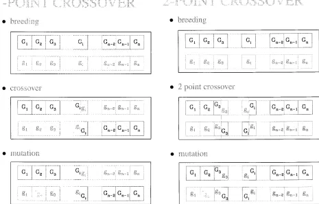
Fig. 2.Schematic view of the main genetic operators acting on two sets of parameter strings in order to procreate two new sets (one chromosome set for each individual) of test strings: natural selection of two individualsGandgfor the breeding of offspring, modification of the genetic content by means of a homologous crossover – at geneGi/gi, and finally the mutation of geneg2to∗g2. Each gene on a chromosome represent a parameter to be optimized. The schematics for a 2-point crossover scheme are shown for comparison
Table 1.PIKAIAcontrol parameters. These parameters were kept fixed at the values listed throughout the evolutionary runs.
initial PIKAIA parameter comment value default identifier
100 100 np the number of individuals per population
20 500 ngen number of generations
2 5 nd number of digits encoding accuracy
2 2 imut mutation mode, imut=2 then pmut=[pmutmn,pmutmx] 0.005 0.005 pmut initial mutation rate
0.005 0.005 pmutmn minimum mutation rate 0.35 0.25 pmutmx maximum mutation rate 0.95 1.0 fdif fitness differential
3 1 irep reproduction plan
0 1 ielite elitism
0 0 ivrb verbose mode
acceptable speed. We refer to Dolphin (1997, 2001, 2002) and Olsen (1999) for a description of a method using SSPs.
2.6.
PIKAIA
ThePIKAIAoptimization package (V1.0; public domain) was developed by Charbonneau (1995) and a full description of this package is given by Charbonneau & Knapp (1996). PIKAIA has been used successfully in a wide range of astrophysical applications (e.g. Bobinger 2000; Charbonneau et al. 1998;
Gibson & Charbonneau 1998; Kaastra et al. 1996; Kennelly et al. 1996; Lamontagne et al. 1996; McIntosh et al. 1998; Metcalfe 1999; Mewe et al. 1996; Noyes et al. 1997; Saha 1998; Wahde 1998).
[image:4.595.118.506.459.619.2]to explore and find in a robust way an optimum, but not nec-essarily the best, setting for a particular problem. In our case this comes down to minimizing the difference between a syn-thetic and an observed CMD by evolving the astrophysical pa-rameters that define the shape of the CMD (see Table 2 and Sects. 2.10 and 3). We follow the generally accepted biological terminology for the description of a genetic algorithm.
A genetic algorithm makes use of a reduced version of the evolutionary process. The gene pool, i.e. the set of parame-ters to be optimized, and its associated phenotypic population evolves in response to
– the reproductive success of the population, following its re-production plan;
– genetic recombination (crossover, see Fig. 2) at breeding;
– random mutations (see Fig. 2) during breeding, which af-fect a subset of the events.
2.6.1. Flow control
PIKAIAhas 12 flow control parameters which are discussed by Charbonneau (1995) to whom we refer for a detailed descrip-tion. We limit ourselves to a short summary and the purposes of these control parameters:npdefines the number of individ-uals in a population;ngenspecifies the number of generations that the population is evolving;ndis number of digits encod-ing accuracy5 used for the parameters;pcross is the proba-bility that a crossover occurs between the chromosomes of the parents;imut,pmut,pmutmn, andpmutmxspecify the muta-tion mode, the mutamuta-tion rate (the initial mutamuta-tion rate if the rate spans the range frompmutmntopmutmxforimut = 2), and the minimum and maximum mutation rate;fdifthe fitness dif-ferential controls the selection of the individuals for breeding through their fitness;irepdefines the reproduction plan to be followed;ielitedefines if the fittest individual can or cannot be selected for replacement; andivrbspecifies verbose mode for extra on screen information during the evolutionary run.
Table 1 holds a list of thePIKAIAflow parameters which were kept constant during all the simulations described in this paper. In the following subsections we describe the extensions added to the 12 flow parameters ofPIKAIA.
2.6.2. Crossover
The crossover operator is very effective in a global exploration of the full parameter space and is in a way comparable to a variational calculus method. A one-point crossover scheme, see Fig. 2, is sometimes inadequate to combine and pass on certain features encoded on the chromosomes (Michalewicz 1996) to its offspring. In some cases only a correlated modification of a number of genes, say 2, will result in a fitter offspring. This can, for example, be mimicked through the application of a two- or multi-point crossover scheme.PIKAIAhas been extended with the control parameterrcrossto handle a multi-point crossover 5 The 1 or 2 number of digits encoding accuracy maps the parame-ter via an integer value, either 0–9 or 0–99, to a range of floating point values by a controlling “normalization” function, see Charbonneau (1995) for additional details.
operation. For example:rcross = 1represents the default one-point crossover, whilercross = 2.3represents a “2.3-point” crossover: i.e. a two-point and three-point crossover for respec-tively 70% and 30% of the cases (2.3=0.7×2+0.3×3).
2.6.3. Brood recombination
An important drawback of genetic algorithms is that the crossover operator is for about 75% of the time lethal to its off -spring, i.e. it produces children which are not as fit as their par-ents (Banzhaf et al. 1998). To avoid missing, potentially, fitter offspring and to reduce the destructive effect of the crossover operator we have incorporated brood recombination inPIKAIA through a new control parameterrbrood. The defaultPIKAIA reproduction scheme is obtained with rbrood = 1, i.e. two parents breed once and produce two new individuals. With rbrood = 3.5 the parents are allowed to breed on average 3.5 times to produce a larger offspring (in this case 7 on av-erage). For rbrood > 1one ends up with more than two off -spring. PIKAIAon the other hand expects from each pair of parents only two children. This constraint was obeyed in or-der not to significantly alter the global behaviour ofPIKAIA. Therefore, in order to avoid an exponential growth of the pop-ulation forrbrood,1, only the fittest two individuals of the local offspring survive6 and enter the global population for a fitness evaluation from which a selection is made for further breeding.
The extra breeding increases the computational effort con-siderably, due to a larger number of function evaluations. The advantage is a more rapid increase of fitter individuals through the selection of effective crossovers from good recombinations. On the other hand, a rapid increase of fitter individuals might lead to a premature convergence to a local minimum, due to a smaller variance in the genetic pool.
2.6.4. Creep mutations
We further introduced the “creep” mutation (Charbonneau & Knapp 1996) in order to overcome the so-called “Hamming Wall” problem, i.e. the inability to cross in a decimal encoding scheme certain boundaries with a one-point mutation operator. The creep parameterpcreepdefines the probability that a gene in the pool undergoes a “standard” mutation (change digit ran-domly in the range 0–9) or the “creep” mutation (add or sub-tract one from the current value of the digit). We adopted as default equal weight for the occurrence of a “creep” or “stan-dard” mutation.
2.6.5. Correlated mutations
an additional way to explore the parameter space like a virus. Although one would prefer to use a (multi-point) crossover op-erator, we do allow that mutations can be used instead, simply because the two operators also co-exist in nature.
We modifiedPIKAIA’s uniform mutation mode. In the ma-jority of the cases we require a (anti-)correlated change be-tween two or more parameters (see Sect. 6.2). In a standard mu-tation scheme convergence might be slow if one has to wait for the simultaneous occurrence of a favourable (anti-)correlated mutation of two specific parameters in order to improve the fit-ness. We introduced an extra parameterpcorrwhich defines the probability that a correlated mutation occurs. If this is not the case the standard mutation scheme is chosen. Otherwise we allowed that in 50% of the cases the mutations of two genes (igen1 and igen2 are extra input parameters added to the modified version of PIKAIA) are more relevant than the mutations occurring in other parameters. For the remain-ing 50% of the cases the two genes are determined stochasti-cally. Additional details about the adopted values of the control parameters are given in Sect. 2.10 and Table A.1.
2.7. Fitness
PIKAIAsearches for the optimum solution by maximizing the fitness functionf. The fittest solution has a fitness f=1, while the worst has f =0. We use the Ng (1998) fitness function, a combination of a chi-squared and Poisson like functions. These functions minimize the differences between observed and syn-thetic diagrams via a star-by-star matching7scheme.
The Ng fitness function is defined as: f = 1
1+F , (1)
whereFis
F=F2χ+FP2. (2)
Fχis the chi-squared function of the best fitted points within a 3–5σerror ellipse andFPis the Poisson function of the resid-ual points outside this ellipse. BothFχandFPare dimension-less, but they hold information about the average uncertainty in units ofσ, sayσχandσP. For example: the average uncertainty per point for a fit withFχisFχ×σχ.
FχandFPare respectively defined as:
Fχ= q
χ2= q
χ2(O,S)/N
match, (3)
and FP=
NO,not+NS,not √
NO+ √
NS
· (4)
The intuitive motive behind this is to make a division between the synthetic points matching the observed CMD for which the errors are expected to be normally distributed and the points which do not match and are allegedly assigned to the Poisson merit function. The method actually usesFχas a loosely fixed 7 This option is feasible due to the increment of the present day computational speed.
“anchor”, puts the outlier points in FP and then reduces the number of unmatched points by minimizingFP. We refer to Ng (1998) for additional details and a discussion of these func-tions. Suffice to say that for an acceptable solution both Fχ
andFPare about 1 or smaller8which on its turn can be relaxed to the conditionF<∼29and thus yields1
3<∼f<1.
The formal 1σk uncertainty of each parameter k, see
Table 4, is obtained through variation of this parameter and by minimizing the function|√Fk−
√
Fmin−1|. Conceptually, this is similar to moving the merit function in theFP,Fχ– plane away from its optimum setting, to the nearest position on a con-tour+1σkhigher. The associated fitness function fσ,k10is:
fσ,k=
1 1+√Fk−
√
Fmin−1
, (5)
wherekis the particular parameter for which the uncertainty is estimated andFmin is the global value obtained for the fittest population.
2.8.
POWELL
We implemented a hybrid optimizer in which we usePIKAIAto explore the parameter space and then usePOWELL’s minimiza-tion algorithm (Powell 1964; Press et al. 1986) to pin down the nearest local or global minimum through a direction set method which producesNmutually conjugate (non-interfering) direc-tions. For details and an excellent description of this algorithm we refer to Press et al. and references cited therein.
A hybrid minimization strategy is used, becausePIKAIAis by definition not a function optimizer, but it tends to get close near a (local) optimum.POWELLis used to get even closer to the (local) optimum. If we had landed in a local optimum then we neededPIKAIAto jump out of it. The origin of our need for a hybrid search strategy is comparable to the minimization problems encountered by Harris & Zaritsky (2001).
2.9. Contracting parameter space
A full exploration of parameter space at one digit accuracy would take considerable time (in the order of weeks), even though certain forbidden combinations of parameters can be excluded `a priori. A full exploration at two or more digits ac-curacy is nearly impossible due to present day computational limits.
We implemented a dynamic, scalable parameter range in our search for an optimum set of parameters. The parameter
8 For our testcase, as described in Sect. 4,F
χranges from 0.7–1.0 for all observed data points with a matching synthetic point within a 3σuncertainty ellipse. This corresponds to a goodness of fit parameter ranging from 0.49–1.0. It further indicates that it is justified to assume that the measurement errors are normally distributed.
9 This condition is comparable but not equivalent to the results ob-tained by Gallart et al. (1999). They demonstrated from a comparison with colour-magnitude bins that a good agreement between the input and recovered SFR(t) required a reduced chi-squared ofχ2
ν'2.0.
Table 2.AMOREcontrol parameters, used as the “educated guess” for the astrophysical parameters in the firstPIKAIAcycle. These values result in a fitnessf=0.004. The value for the parameters are constrained between the lower and upper limit.
# parameter value lower limit upper limit description
1 logd 3.7 3.6 4.0 log of distance
2 AV 0.30 – 0.001 0.5 extinction
3 logtlow 9.5 9.0 10.3 log lower age limit
4 [Z]low – 0.90 – 1.69897 0.69897 log lower metallicity limit
5 α 1.35 1.001 3.5 IMF slope
6 logthigh 9.6 9.0 10.3 log upper age limit
7 [Z]high 0.30 – 1.69897 0.69897 log upper metallicity limit
8 β 1.0 – 2.00 5.00 SFR slope
range shrinks after each optimization cycle withPOWELL. This leads to an improved accuracy in the results with a fixed num-ber of digits encoding accuracy.
The automated re-scaling of the parameter range improves the resolution of the exploration of the search grid. In addition, due to the re-scaling one may circumvent partial degeneracy of the parameters.
The global functionF(Fχ,FP) gives the global distance to the minimum in terms ofσ2(σχ, σP). If we havenparameters then each parameterkis in a simple approach on average about √
F/nσkaway from its optimum value, because we assume that
F=
n
X
k=1
yk,sim−yk,true σk
!2
, (6)
whereyk,sim is the simulated value of parameter kandyk,true is the true value of parameterk. The average offset per pa-rameterkis therefore √F/n. The new limits can then be set to ±√F/nσk. To balance the cancellation of errors, due to
a negative correlation between some parameters, we adopt a rather conservative approach by constraining the limits of each parameterkto±3×1.3√F/nσk. In addition we add the
con-dition that 3×1.3√F/n>0.005.
2.10. Adjustable parameters: Free and fixed
AMORE uses in essence two different sets of parameters as input. One set contains program flow control parameters and information about the observational data to be simulated: the photometric errors and crowding factors per passband, a shift of the zeropoint of the colours due to a difference between the observed and synthetic photometric system, and the spread around the average extinction value to account partly for the differential reddening in a field.
The other set of input parameters is used byPIKAIAand can be divided into two parts (see Tables 1 and 2). One part contains thePIKAIAcontrol parameters. The other part con-tains the lower and upper limits of the astrophysical parame-ters to be optimized as well as an initial guess for the value of those parameters (first column of Table 2, resulting HRD in Fig. 6b). These parameters are a combination of the synthetic population’s intrinsic properties, i.e. age, metallicity, slope of the power-law IMF and the index of the exponential SFR.
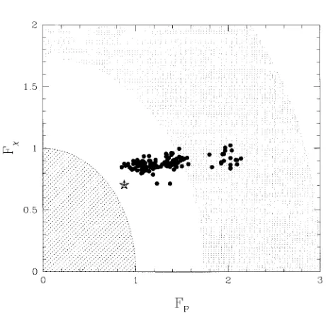
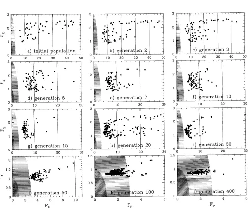
Fig. 3. Evolutionary status for all the trial models (filled dots; see Table A.1 for details) for each population after 400 generations, see also Fig. 4. The filled starFpoints to the location obtained with the original parameter settings as given in Table 4. Acceptable solutions are found in the region for which both Fχ and FP are less than 1, see Sect. 2.7. The condition has been relaxed toF<2 (solid white line). The asterisk indicates the position obtained for a different re-alisation of the test population by changing the random seed. The shaded regions indicate solutions for which the difference between the CMDs from the “observed” and synthetic population is on average less than respectively 3σ,√3σ, and 1σ. Note that rounding errors, see Sects. 5.1.1 and 6.3, give rise to a degeneration of the parameter space around f>0.25 (i.e.F<3).
In our case we allow for age and metallicity not to be restricted to one fixed value, but to cover a specific range (see Table 2).
In addition, there are two parameters which mimic the syn-thetic population’s behaviour as placed in a mockup version of our Galaxy. These parameters are the distance from the Sun and the average extinction.
[image:7.595.298.528.230.451.2]3. Method
3.1. Genetic evolution
In terms of genetic programming the objective ofAMOREis to determine the genome (i.e. the set ofastrophysical parameters described in Sect. 2.10, see also Table 2) of a specified indi-vidual (i.e. theobserved stellar population). Note that it is not possible to directly observe the genome. The genome is deter-mined from the phenotype of each individual (i.e. thesynthetic CMDs, see for example Fig. 6). The genetic information is lo-cated in the genes of one chromosome11.
A guess of the genotype of the observed CMD is obtained through comparison with a synthetic CMD, which is gener-ated via supervised evolution and breeding (PIKAIAtogether withPOWELL). The stars in the synthetic CMD population with a particular genotype are raised to maturity (HRD-ZVAR and HRD-GST). A group of individuals12 is allowed to procreate (the chance of an individual procreating depends on its fit-ness and the selection pressure, see Charbonneau 1995 and Charbonneau & Knapp 1996) and the genetic information of the parents is passed on to their offspring (see Fig. 2).
A fitness evaluation (a comparison between the observed and synthetic CMD) provides a ranking of the resulting group of individuals. If the individual has “good genes” it survives, remains in the group and gets a chance of procreation.
The evolutionary process of breeding and fitness evaluation is repeated for a fixed number of generations. The gene pool of the resulting best individual at the end of the evolutionary run with AMORE hopefully represents a near-optimum represen-tation of the unknown genome.
3.2. Running AMORE
Initially PIKAIA is in control (see Fig. 1) of the evolution for a fixed number of generations. Afterwards POWELL tries to improve the genome of the fittest individual communicated throughPIKAIA. We then determine the uncertainty for each gene on the chromosome. Subsequently, we tighten the limits on the range of variation allowed for each gene and re-scale the parameters on the genetic print of the fittest individual accord-ingly. During the shrinkage of the parameter range we do not re-scale the genetic information of the remaining individuals, but preserve their former values as semi-random input for the continued optimization process. The latter addition to the hy-brid scheme is most likely a significant driver in speeding up the search for a fitter individual.
After each optimization with POWELL a new cycle with PIKAIA is started with the current best parameter set as “ed-ucated next guess” for AMORE’s progressive evolution. The total number ofPIKAIAcycles is user defined.
11 The genetic information is currently located on one chromosome. Individuals with two chromosomes might be considered as a future extension. A two-chromosome approach has the advantage that certain genetic information can remain present in a recessive form.
12 To avoid confusion the termgroupis used instead of the biological termpopulation, because each individual in the group is actually a synthetic stellar population.
In Sect. 2.9 we argued that the parameters are on average about √F/nσkaway from its optimum value. The convergence
however is not governed by the average “distance” that each parameters is away from its optimum setting. It is mainly de-termined from the ability to tune the parameter which has the largest offset from its optimum value.
In the AMORE training sessions it was noted that with F'3.0 about three of the eight parameters are about 1σk
(' √F/3σk) away from their optimum value.AMOREhas a
built-in option to do a random variation from 0–3σk of two
parameters (randomly selected) from the running best solution when the fitness is less than 0.30. Above this threshold we choose a new value for two parameters according±pF/ρ σk,
whereρcan be any number between 1.0 and 4.0.
4. Tests
4.1. Test objectives
We performed several tests onAMOREin order to
– verify and validateAMORE’s performance in retrieving the astrophysical parameters of a synthetic single stellar popu-lation;
– determine adequate values for the parameters pcross, rcross, rbrood, pcreep, and pcorrin the extended version ofPIKAIA;
– study the effects of rounding and degeneracy;
– study the effects of fixing parameters on the convergence.
4.2. Setup
The hybrid interaction betweenPIKAIAandPOWELL, combined with a progressive shrinking/re-scaling of the parameter space, requires that a trade-offhas to be made in the choice of the size of the population and the number of generations we allow this population to evolve in order to obtain results in a reasonable amount of CPU processing time.
We explored several different settings for thePIKAIA con-trol parameters, because the tuning of those parameters is very problem dependent (Charbonneau & Knapp 1996). The val-ues we decided to use are listed in Table 1. Four notes can be made here.
Firstly the steady-state-delete-worst reproduction plan (irep=3) we adopted, in which we replace the least-fit vidual from the population when the fitness of the new indi-vidual is superior to that of the least-fit population member. Choosing this reproduction plan implies that the elitism con-trol parameter (ielite) is non-operative, because elitism is active by default. We evaluated two other reproduction plans (Charbonneau & Knapp 1996); full generational replacement and steady-state-delete-random. The steady-state-delete-worst reproduction plan produced on average the best results.
Secondly the mutation rate of 0.35 corresponds, in case of a default 2 digit accuracy, with the on average occurrence of 2.8 mutations per astrophysical parameter.
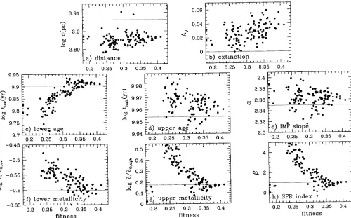
Fig. 4.The filled circles in panelsa)–f)display the values obtained for the parameters using the models in Table A.1. The solid line refers to the value set for the original population.
(Charbonneau & Knapp 1996). Settingfdif=0.95 turned out to be a good trade-offchoice.
Fourthly, we want to explore as large a fraction of the pa-rameter space as possible at the first entry inAMORE. This is done by using only an one digit accuracy (nd=1). Due to the active re-scaling of the parameter space boundaries we do not require a very high precision in our exploration. A one percent accuracy (nd=2) of the parameter space is sufficient in the sub-sequentPIKAIAcycles.
In biological terms, thePIKAIAcontrol parameters define the ecosystem in which our population evolves.
All computations presented in this paper were performed with an executable generated with the g77 compiler. This executable was then installed on various PCs running Red Hat Linux13 6.X and 7.X. The PCs were equipped with Intel Pentium III or Athlon processors with clock speeds ranging from 600 – 1200 MHz.
All tests, unless stated otherwise, use the synthetic popula-tion as described by Ng (1998):
− a metallicity range, spanningZ=0.005–0.030; − an age range from 8–9 Gyr;
− an initial mass function with a Salpeter slope;
− an exponential decreasing star formation rate with a char-acteristic time scale of 1 Gyr.
13 Red HatRis a registered trademark of Red Hat Software, Inc. and LinuxRis a registered trademark of Linus Torvalds.
Table 3.Average fitness (fA) for different values of the parameters as obtained from Table A.1. The first column displays the parame-ter name which is varied, the parameparame-ter value is given in the second column, the third & fourth column show respectively fA, uncorrected forpcorr=0.0, together with its standard deviation, and the fifth and sixth column display the averaged values after removal of the results of the models withpcorr=0.0. See Sect. 5.1.2 for additional details.
parameter value fA σn−1 fA σn−1 pcross 0.50 0.276 0.070 0.287 0.066
0.85 0.299 0.063 0.297 0.056 rcross 1.00 0.293 0.065 0.290 0.063 2.00 0.285 0.068 0.297 0.065 3.00 0.285 0.070 0.290 0.057 rbrood 1.00 0.286 0.077 0.230 0.059 2.00 0.292 0.058 0.301 0.055 4.00 0.285 0.066 0.276 0.067 pcreep 0.0 0.287 0.071 0.292 0.068 0.3 0.290 0.065 0.297 0.058 0.7 0.285 0.066 0.288 0.060 pcorr 0.0 0.278 0.077 NA NA
0.3 0.285 0.065 NA NA 0.7 0.300 0.057 NA NA
[image:9.595.307.520.511.688.2]4.3. Description of the tests
4.3.1. Test 1: Determining values for
pcross,
rcross, rbrood, pcreep,
andpcorr
In the first test, we evaluate the 162 models listed in Table A.1 in order to study the effect of thePIKAIAparameterspcross, rcross, rbrood, pcreep, and pcorron the convergence and computational effort. The test has as a secondary objective to provide an understanding of the degeneracy of the parameter space.
All astrophysical parameters to be retrieved are set free, floating between reasonable minimum and maximum val-ues (see Table 2 for details).AMORE runs for 20 iterations of 20 generations (ngen=20) to recover the a priori known pa-rameters of the synthetic population. The number of iterations and generations determine the total length of an evolutionary run: 20×20 = 400 generations. Note that the range of each parameter is set within reasonable limits and not taken exces-sively large, because it might lead to the case that no acceptable parameter setting is found with the standard iteration loop.
4.3.2. Test 2: Rounding
The second test deals with the effects of rounding. We vary the number of significant digits in the input parameters to reveal
AMORE’s sensitivity to rounding. In this case we do not make an evolutionary run, because the trial set of parameters (the ed-ucated guess at the start-up of a PIKAIAcycle) is the correct one. For clarity we label the fitness in this test by ftrialinstead of fA, the fitness after a complete evolutionary run.
4.3.3. Test 3: Fixing parameters at the correct value
In the third test we take six models in which one of the pa-rameters is set fixed at its correct value in order to study the effects on the convergence. The models chosen were two of high, two of intermediate and two of low fitness as determined from the first test. The convergence in this test basically can go two ways: either the convergence is faster, because less pa-rameters have to be optimized. Or, due to the fact thatAMORE
has less maneuverability in this situation, the convergence is slower. We adjusted the limits for age and metallicity as given in Table 2 such thatAMOREwould not try to find solutions in forbidden regions of parameter space which might severely slow down convergence due to constant rejection byAMORE
of the chosen parameter values.
For example, fixing the [Z]lowparameter at its correct value of – 0.60206 means that we have to adjust the lower limit for [Z]highto – 0.60206 as well.
In the case of fixing the logtlow parameter this also im-plies that the initial guess has to be adjusted. We set this initial guess to 10.1.
4.3.4. Test 4: Fixing parameters at the wrong value
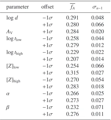
In the fourth test we take six models in which one of the parameters is set fixed at 1σ offset (determined from the
first test) from its original value, in order to study its effect on the “second best” setting of the remaining parameters. Normally one would expect a fitness f>1
3. In this case, however, F < F2
P +F 2
χ = 12 +(1+1)2 = 5 and the
as-sociated fitness constraint drops to f>16. However, this assessment ignores the fact that, when a parameter is offset from its optimum value, the number of matched points will decrease and FP increases. Using Eq. (6) one has for a good fit F = 2. On average the offset per parameter k from the optimum value is
q 1 4σk =
1
2σk, at best the offset is 0σk, and in the worst case this is √2σk. So with one parameter
k put at 1σk offset we distinguish the three possibilities
1 at best F=(1+2) =3 → f=14
2 on average F=(1+1 2)
2+7
4 =4 → f=
1 5 3 at worst F=(1+√2)2 =5.8 → f= 1
6.8· Note that the worst case limit is in agreement with the results presented in Table A.3.
The effect of the 1σ offset of one of the parameters will partly be canceled by forcing other parameters away from the optimum value. For example, the effect of an increased extinc-tion can be masked partially by generating a bluer stellar pop-ulation with a lower metallicity and a younger age. The effect will be such that the fitness will not be aroundf'61.8, but some-where in the range61.8<f<13·
We fixed the parameters both at one sigma above and one sigma below the original value, because the evolutionary ef-fects do not have to be symmetric. The only exception is the extinction, which we only fix at one sigma above the original value ofAV =0.0.
Again we adjusted the limits for the upper and lower limit for age and metallicity.
5. Results
AMOREhas been tested for a wide range of setups. The results in Table A.1 indicate thatAMORE give both acceptable and less acceptable solutions. They are displayed in Figs. 3 and 4.
[image:10.595.322.559.220.261.2]To better understand what goes on during the genetic evo-lution we display the results from model A.1-40. Figure 5 dis-plays an example of the evolution of the merit functionF for a number of generations. It shows how the initially dispersed individuals gradually find their way, start to cluster together around generation 10, and penetrate the region with acceptable solutions after about 50 generations. After 100 generations the improvements become marginal for this model.
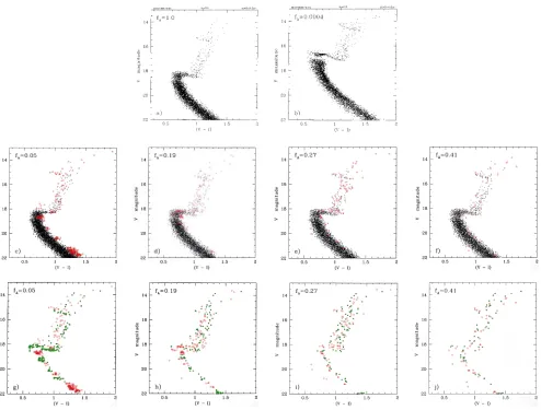
Figure 6 displays for the same model A.1-40 the phenotypi-cal changes of the CMD for several fitnesses during the genetic evolution. The various panels show that the synthetic CMD re-sembles better and better the “observed” CMD when the fitness improves. Note that at fitness f=0.05 one already gets for the eye appealing solutions.
Table 4.The effect of rounding in the parameters on the fitness evaluation; ftrialis the fitness obtained withAMOREfor the given values of the parameters. Theaverage valueandσare based on the 162 models in Table A.1. Theσis obtained from an unweighted average for the fitness of the models involved. Thebσis the error as estimated by Ng 1998.
parameter logd(pc) AV logtlow logthigh [Z]low [Z]high α β ftrial original 3.906335 0m.00 9.90309 9.95424 – 0.60206 0.17609 2.35 1.0 0.44597 round-v1 3.906 0m.00 9.903 9.954 – 0.60 0.18 2.35 1.0 0.28595 round-v2 3.906 0m.00 9.903 9.954 – 0.602 0.176 2.35 1.0 0.30812 round-v3 3.9063 0m.00 9.9031 9.9542 – 0.602 0.176 2.35 1.0 0.42439 average value 3.8958 0m.027 9.866 9.984 – 0.554 0.244 2.358 1.574
σ 0.0033 0m.014 0.049 0.047 0.050 0.13 0.034 1.40
bσ 0.012 0m.06 0.043 0.023 0.18 0.08 0.03 1.4
[image:11.595.33.538.243.666.2]the astrophysical parameters obtained from model A.1-40 get quite close to the parameters of the CMD to be matched.
5.1. Test 1: Parameter values and degeneracy
5.1.1. Degeneracy of the parameter space
Table A.1 is displayed in Fig. 3. The clustering in the figure provides an indication that a degeneracy of the parameter space is present near f>0.25 (i.e.F<3, see Eq. (1)). Without a ma-jor computational effort it will be difficult to obtain a significant improvement of the parameters once f>0.25. However,F<3 indicates a region in the (Fχ,FP)-plane for which the system-atic offset of the individual parameters from its true value are on average less than √F/nσk=0.6σk, see Sect. 2.9 for details.
In practice it turns out that a strong correlation between three of the eight parameters has the culprit; at least two of them have to change simultaneously in the proper direction in order to improve the fitness (see also Sect. 6.3). They have an average offset of∼√F/3σk=1σk, while for the remaining parameters
this is1σk.
In addition, Fig. 4 displays the retrieved parameters for all models as a function of fitness. Note, that AMORE systemat-ically underestimates the distance of the test population. On the other hand, the effect of this underestimation is in its turn partially canceled by overestimating the extinction, the upper age limit and the slope of the power-law IMF slightly (see also Fig. 7). Another clue we get from Fig. 4 is that the slope of the SFRβis very poorly constrained.
5.1.2. Determining values for
pcross, rcross,
rbrood, pcreep,
andpcorr
Looking at Table A.1, a result that is immediately obvious is thatpcorr=0.0 has a strong stabilizing effect on the simula-tion. Its effects overwhelm the effects of thepcreepparameter and lock fAat a certain value, which may be quite good (e.g. models 10, 11 and 12) or quite poor (e.g. models 28, 29 and 30). Settingpcorr>0 is thus preferred to avoid getting locked in a low value for fA.
In order to compensate for this strong stabilizing effect, we also evaluate in Table 3 the average fitness of the models when we exclude all models which havepcorr=0.0.
As expected, therbroodparameter has a strong influence on the amount of computational time needed. Although the models with high values of rbrood are somewhat better than models with low values, this effect is only marginal. Considering that a high value of rbrood lessens the genetic variation in the gene pool while increasing the computational time needed for a run with several factors, it is desirable to have a low value ofrbrood.
[image:12.595.377.513.133.268.2]The different parameters are not independent, as can be seen from Table A.1 and Table 3. Simply taking the best options in Table 3 yields model 134 for the case in which pcorr=0.0 has not been corrected for, a reasonable, but not an exceptionally good model.
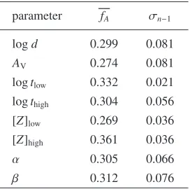
Table 5.Fitness statistics when fixing one parameter at its correct value. Averaged fitness values fA and their associated standard de-viationσn−1are obtained from simulations with the setup parameters from models 9, 14, 22, 34, 40 and 52. See Table A.2 for additional details.
parameter fA σn−1 logd 0.299 0.081
AV 0.274 0.081
logtlow 0.332 0.021 logthigh 0.304 0.056 [Z]low 0.269 0.036 [Z]high 0.361 0.036
α 0.305 0.066
β 0.312 0.076
5.2. Test 2: Rounding
Table 4 shows the effect of the accuracy of the retrieved val-ues of the parameters on the evaluation of the fitness. If one applies a rounding to one or two significant digits it is not pos-sible to reproduce the expected fitness, i.e. the expected fitness drops from ftrial=0.44 toftrial=0.28. A better agreement can be obtained by reporting the values of the parameters with the addition of one or more (apparently insignificant) digit(s). A renewed search (Table 4; round-v3) circumvents the local op-timum at ftrial = 0.28 and results in a near global fitness of
ftrial=0.42, which is close enough to the value expected. Thetrueσline in the table shows that both the [Z]highand theβparameter are the weak links in the overall parameter es-timation (see also Fig 4).
5.3. Test 3: Fixing parameters at the correct value
The results of fixing parameters at the correct value are listed in Table A.2 and an example of the diagnostics is listed in Table 6. Details of the individual setups for these tests are given below. In general, the results of the tests for which one of the param-eters was set to the correct value were slightly better than the results for the models for which all parameters are set free, see Tables 4 and 5 for additional details. This behaviour is due to the fact that by forcing one parameter to a fixed value the evo-lutionary path changes. The models were selected from the re-sults with low and intermediate fitness given in Table A.1.
5.3.1. Fixed distance and extinction
Distance and extinction are negatively correlated. When both parameters are set free, a certain degree of degeneracy is to be expected. Fixing one of the parameters at its correct value can break this degeneracy. The result depends strongly on the evolutionary path of the other parameters.
Fig. 6.Genetic evolution of the colour-magnitude diagram (CMD) from the first test population. Panela)displays the original population to be matched. The physical parameters for this population are described Table 2 and Sect. 4.2. The CMD of the initial trial population is shown in panelb). Panelsc)–e)display the resulting CMDs obtained with setup A.1-40 for different fitnesses (see Sect 2.7). The fitnesses f =0.05, f=0.19 andf =0.27 are respectively reached after 20, 60 and 80 generations. The dots in the panelsb)–e)are used for each matching point, while the red open starsFin panelsc)–j)are the points in the simulation which have no counterpart in the original CMD. Panelf)displays the fitnessf =0.41 as obtained after 341 generations. Note that the CMDs of panelsa)andf)as well asc)–e)are visually almost indistinguishable. Panelsg)–j)displays the residuals between the simulated and the original CMD (a; green solid squares) are those points in the original which have no counterpart in the simulation.
age-metallicity degeneracy. Excluding this value results in an average fitness offA=0.328±0.039. In general: the extinction can be reliably retrieved when fixing the distance.
When considering a fixed extinction, the results show a strong variation in both age and metallicity. It should also be noted that the average10log (distance (pc)) retrieved is only 3.8953±0.0066. This is more than one sigma away from the optimum value for the distance (see Table 4). This is an in-dication that retrieval of the distance by fixing the extinction is hampered by the age-metallicity degeneracy. Therefore, the distance cannot be reliably retrieved when fixing the extinction to its correct value.
5.3.2. Fixed age and metallicity
Fixing one of the age limits results in values for both the age and metallicity which are close to the input values. This is due
to the (partial) breaking of the age-metallicity degeneracy. The distance-extinction degeneracy remains. The results also sug-gest that the age-metallicity degeneracy has a stronger impact on the fitness than the distance-extinction degeneracy.
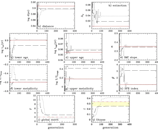
Fig. 7.Panelsa)–h)display the convergence curves for the parameters of models A.1-40 (dotted line; fitnessf =0.41) and A.1-51 (long dashed line; fitness f =0.25). The solid line in the framesa)–f)refers to the value adopted for the original population. The long, dot dashed line in framesi)andj)shows the threshold values to be crossed for acceptable solutions, i.e.F<2 and 1
3<f<1. The short dashed area in framej) marks the region where degeneracy of the parameter space becomes noticeable (see Sects. 6.3 for details).
limit can be better determined when both the low and high lim-its are determined in union.
5.3.3. Fixed slope for the power-law IMF
Fixing the slopeαof the power-law IMF to its correct value ensures stability in the magnitude direction of the CMD. This implies that the degeneracy in the colour dependent parame-ters, like age, metallicity, and partly the star formation rate, be-comes more apparent. Although the overall results are quite good, only model A.2-14 is significantly affected by this de-generacy. If we leave out model A.2-14 from the statistics the average fitness becomesfA=0.331±0.020.
5.3.4. Fixed slope for the exponential SFR
The exponential star formation rate parameterβis tied to the age and metallicity range, see also Sect. 5.3.2. Fixing the pa-rameterβbetter constrains in particular the upper metallicity limit. However, it does not avoid that the genetic evolution en-ters into a local age-metallicity gap, see Table A.2. Excluding model A.2-34 improves the average fitness in Table 5 to
fA=0.342±0.029.
5.4. Test 4: Fixing parameters at the wrong value
Table 6.Description of the diagnostic statistics for model A.1-40 when fixing one parameter at its correct value, see Sects. 5.3, 2.7 and 6.2.1 for additional details.
model NO,not NS,not Nmatch Fχ FP F fA
ideal 0 0 5000 0.000 0.000 0.000 1.000
free 60 60 4940 0.847 0.849 1.438 0.410
fixed: logd(pc) 155 155 4845 0.903 2.192 5.621 0.151
fixed:AV 103 103 4897 0.840 1.457 2.827 0.261
fixed: logtlow(yr) 76 76 4924 0.817 1.075 1.823 0.354 fixed: logthigh(yr) 104 104 4896 0.902 1.471 2.978 0.251
fixed: [Z]low 94 94 4906 0.836 1.329 2.466 0.289
fixed: [Z]high 76 76 4924 0.815 1.075 1.820 0.355
fixed:α 74 74 4926 0.834 1.047 1.799 0.357
fixed:β 80 80 4920 0.727 1.131 1.808 0.356
Table 7.Fitness statistics when fixing one parameter ±1σfrom its original value. Averaged fitness values fAand their associated stan-dard deviationσn−1are obtained from simulations with the setup pa-rameters from models 9, 14, 22, 34, 40 and 52. See Table A.2 for additional details.
parameter offset fA σn−1 logd −1σ 0.291 0.048
+1σ 0.280 0.066
AV +1σ 0.284 0.020
logtlow −1σ 0.258 0.044 +1σ 0.279 0.012 logthigh −1σ 0.229 0.022 +1σ 0.207 0.014 [Z]low −1σ 0.254 0.066 +1σ 0.315 0.027 [Z]high −1σ 0.270 0.054 +1σ 0.283 0.018
α −1σ 0.266 0.025
+1σ 0.273 0.027
β −1σ 0.232 0.071
+1σ 0.276 0.011
5.4.1. Erroneous distance
A wrong assumption about the distance gives in a vertical shift in the CMD (all other parameters give a diagonal shift) and cannot be masked out through a correlated change of any of the other parameters. This results in quite a wide range in the values of the other parameters, except the value ofα. The un-expected result is that irrespective if the distance is too short or too far: the power-law IMF slope flattens!
If the distance is overestimated there are more synthetic stars present at fainter magnitudes. To get relatively more syn-thetic stars at brighter magnitudes one needs to flatten the power-law IMF slope.
If the distance is underestimated then more synthetic stars are present at brighter magnitudes. One expects that a steeper power-law IMF slope is required as compensation. This is not always true, see Table A.3. Stars pop up at the lower end of the main sequence. They are taken away from the stars located at
brighter and brighter magnitudes. One therefore requires also in this case a flatter IMF slope.
A flatter slope of the power-law IMF can be a hint that the distance of the stellar aggregate is wrong. Or it might be a hint that the zero point of the adopted synthetic photometric system is different from the actual photometric system used.
Recognizing that the slope is indeed flatter than the ma-jority of the other cases outlined in Table 4 one may start to explore the assumption that the distance is wrong: release the constraint during the next exploration.
The sensitivity to the distance implies thatAMOREcan be used to determine the distance to a stellar aggregate quite reli-ably. A bonus is that due to an initially wrongly assumed dis-tance the extinction is in most cases better constrained.
5.4.2. Erroneous extinction, age and metallicity
In (V, V−I) CMDs a strong correlation between extinction, age and metallicity exists (see also Ng & Bertelli 1996 and references cited therein). A higher value of the extinction can be compensated by a younger age and/or a lower metallicity. Indeed, the results in Table A.3 show that this actually oc-curs for the lower age and metallicity limit. The upper age and metallicity limit, however, drifts away in the opposite direc-tion to compensate for “erroneous correcdirec-tions” applied by other parameters.
A higher value of the star formation index results in a lower number of stars at the upper age metallicity limit. To get a suf-ficient number of high metallicity stars one has to stretch the upper metallicity limit to a slightly higher value.
We further notice that a wrong value for the age and met-allicity does not affect the extinction significantly. Our find-ings indirectly supports the method to determine high resolu-tion (40×40) extinction maps towards the Galactic bulge by Schultheis et al. (1999) with the data obtained for the DeNIS project (Epchtein et al. 1997).
5.4.3. Erroneous slope for power-law IMF
[image:15.595.65.242.321.512.2]extremely large. The slightly larger value of the slopeαpushes slightly more synthetic stars to fainter magnitudes, introduc-ing a relative deficiency of stars at brighter magnitudes. This is compensated through a younger age, a decrease of the lower metallicity limit and an increase of the upper metallicity limit. The higher value for the upper age and metallicity limit com-pensates in its turn for the overestimation of the exponential star formation index.
A lower value ofαis partly compensated for by lowering the upper age limit, lowering the lower metallicity limit and overestimating the upper metallicity limit.
5.4.4. Erroneous index for exponential SFR
A larger index for an exponentially decreasing SFR pushes more stars of the population to the blue edge of the CMD, re-sulting in a slightly bluer stellar population.AMORE compen-sates this by mainly increasing the upper metallicity limit, i.e. reddening the synthetic stellar population.
A lower value for the SFR index has the opposite effect.
AMOREcompensates for the now slightly redder population by lowering the upper metallicity limit, making the population bluer.
6. Discussion
6.1. Relative contribution of the parameters to the fitness
Figure 4 and the Tables 4, 5, 7, A.2 and A.3 provide the hint that not all parameters have an equal contribution to the fitness. It appears that theβand [Z]highparameter can vary considerably and still yield a decent fitness. Moreover, Tables A.2 and 5 indi-cate that knowledge of the value of the [Z]highparameter results in acceptable values for the other parameters.
The origin of this behaviour lies in the implicit definition of the exponential star formation rate (forβ=1 one has a decreas-ing star formation towards a younger age) attached to a linear age-metallicity relation. The latter relation will give less metal-richer stars. The small number of stars with higher metallicity induces a larger variation of the [Z]highparameter without af-fecting significantly the overall fitness.
6.2. Convergence
The fine-tuning of the genetic algorithm is a tedious task. It is not straightforward to find the optimum setting for the problem to be solved. One has to balance the exploring qual-ity through crossovers against the variation of the parameters through (creep) mutations.
We did not want to deal with a mutation dominated search, because it tends to move farther away from an optimum pa-rameter setting in the majority of the cases. We used therefore a relatively high crossover probability (pcross) and we set the mutations at a fixed rate, such that on average only 2.8 muta-tions occur in the gene pool of each individual.
At a certain stage however one requires the variation of other correlated parameters to obtain an improvement. This
becomes particularly necessary when approaching the opti-mum setting of the parameters. A favourable crossover and mu-tation might do the trick, but it might take a while before this occurs. We introduced in Sect. 2.6.5 the possibility that two parameters might be more sensitive to mutations than others. This approach gave better results for the majority of the trial cases (see Table 3), but it failed to obtain improvements when changes of one parameter were neutralized through the vari-ation of one or more parameters. The distance-extinction and the age-metallicity degeneracies slow down the convergence ofAMOREforf >0.3, see Fig. 4.
One of the modifications to consider for future implemen-tation is a two-chromosome approach. In that case acceptable values for the parameters do not shift out of the population if the overall fitness is less, but still reside in the gene pool as a recessive quality. This however, will require a major exten-sion toPIKAIAand a significant amount of genetic research to be done about dominant and recessive qualities in theAMORE
gene pool.
Another modification to consider in order to improve the ac-curacy and to speed up convergence, is to replace the finite resolution of the digital encoding scheme with a genetic cod-ing based on floatcod-ing point, i.e. each gene on the chromo-some is represented by one floating point number. According to Michalewicz (1996) a real encoding scheme can be superior and improve convergence. Such an encoding scheme is indeed to be included in the next release ofPIKAIA2.0 (Charbonneau; in preparation).
6.2.1. Unstable solutions
In one test (fixing AV at one sigma above the original value for model 9) no convergence was achieved and the run was aborted. BecauseAMOREis quite sensitive to rounding these effects can be circumvented by slightly altering the input pa-rameters. We decided in this case against such an action, be-cause that would make the sample inhomogeneous.
6.3. Degeneracy
Table 8.Description of the diagnostic statistics for simulations with setup parameters from model A.1-40. One of the parameters is forced to a value±1σfrom its original value. See Sects. 5.4 and 2.7 for additional details.
model offset NO,not NS,not Nmatch Fχ FP F fA
ideal 0 0 5000 0.000 0.000 0.000 1.000
free 60 60 4940 0.847 0.849 1.438 0.410
fixed: logd(pc) −1σ 91 91 4909 0.788 1.287 2.278 0.305 +1σ 85 85 4915 0.722 1.202 1.967 0.337 fixed:AV +1σ 98 98 4902 0.932 1.386 3.790 0.264 fixed: logtlow(yr) −1σ 91 91 4901 0.897 1.287 2.460 0.289 +1σ 94 94 4906 0.905 1.329 2.587 0.278 fixed: logthigh(yr) −1σ 106 106 4894 0.977 1.499 3.202 0.238 +1σ 126 126 4874 1.017 1.782 4.211 0.192 fixed: [Z]low −1σ 78 78 4922 0.907 1.103 2.043 0.329 +1σ 80 80 4920 0.835 1.131 1.977 0.336 fixed: [Z]high −1σ 148 148 4852 0.896 2.094 5.188 0.162 +1σ 94 94 4906 0.867 1.329 2.519 0.284 fixed:α −1σ 95 95 4905 0.886 1.344 2.590 0.279 +1σ 103 103 4897 0.894 1.457 2.921 0.255 fixed:β −1σ 145 145 4855 0.930 2.051 5.071 0.165 +1σ 103 103 4897 0.834 1.457 2.818 0.262
extinction does not automatically imply that the distance can be retrieved accurately.
As demonstrated in Sect. 5.1.1 the degeneracy among pa-rameters becomes noticeable for f >0.25 orF<3. This cor-responds to systematic offset for each parameter of on aver-age∼0.6σkand at maximum∼1σk. The Poisson uncertainty of
the original population results in a fitness off=0.43 (F'1.33). However, solutions with a comparable fitness do exist due to the degeneracy of the parameter space. A direct consequence is that there is an intrinsic offset present among the parame-ters amounting to on average∼0.4σkand at maximum∼0.7σk.
This intrinsic offset is present in the solutions obtained with
AMOREand actually is responsible for slowing down the con-vergence in the fitness range 0.30< f <0.43. It will therefore be nearly impossible to recover in one pass the original input values. However, some improvements might be obtained by av-eraging the parameter values obtained fromAMOREruns with different initial conditions.
7. Conclusions
We demonstrate that an automatic search can be made for the astrophysical parameters of a synthetic stellar population from the analysis of colour-magnitude diagrams with an opti-mizer, based on a genetic algorithm. However,AMOREtends to slightly underestimate the distance. It subsequently attempts to compensate this with an higher extinction, a higher upper age and a slightly steeper slope for the power-law IMF. At f >0.3 the combined effect of the age-metallicity and the distance-extinction degeneracy slows down the convergence. The data suggests thatAMOREhas more problems dealing with the age-metallicity than with the distance-extinction degeneracy. For general purpose, however, the retrieved values are sufficiently accurate.
8. Future work
The good results obtained so far for a single synthetic stellar population is an indication aboutAMORE’s potential for the detailed analysis of CMDs. The next step is to improve one step at a time various aspects ofAMOREbefore it can be used as an interpretative tool for large photometric surveys.
Despite limitations in the input physics of the underlying stellar evolutionary tracks and by the transformation from the theoretical to the observational plane, the results with real data from Gallart et al. (1999), who uses the same set of evolu-tionary tracks, are encouraging. It will therefore be important to verify first with, for example, well studied open clusters (see Carraro et al. 1998, 1999 and references cited therein) for which age and metallicity range we may applyAMOREsafely. Extinction is also of some concern, because a high extinction may result in the MS turnoffpoint to fall below the detection limit. This would depriveAMOREof a clear reference point.
Another case of interest is of course the question how many different stellar populations can be distinguished with
AMORE. Separating multiple, mixed populations from each other through the automated and the objective analysis of colour-magnitude diagrams could be a valuable tool for the analysis of galaxy formation and evolution.
This requires a rigorous follow up study on the separation of multiple (synthetic) populations. One further ought to verify if the automated analysis of colour-colour diagram can reduce the effects of error cancellation between distance and extinc-tion.