A Modified Centered Climbing Algorithm for Linear
Programming
Ming-Fang Ding, Yanqun Liu, John Anthony Gear
School of Mathematical & Geospatial Sciences, RMIT University, Melbourne, Australia Email: [email protected]
Received July 9, 2012; revised August 9, 2012; accepted August 16, 2012
ABSTRACT
In this paper, we propose a modified centered climbing algorithm (MCCA) for linear programs, which improves the centered climbing algorithm (CCA) developed for linear programs recently. MCCA implements a specific climbing scheme where a violated constraint is probed by means of the centered vector used by CCA. Computational comparison is made with CCA and the simplex method. Numerical tests show that, on average CPU time, MCCA runs faster than both CCA and the simplex method in terms of tested problems. In addition, a simple initialization technique is intro-duced.
Keywords: Linear Programming; Ladder Method; Climbing Rules; Simplex Method
1. Introduction
In the last decades a variety of algorithms have been pro- posed for solving linear programming (LP) problems (see, e.g., [1-5]). However, so far there hasn’t been an avail-able single best LP algorithm which is suitavail-able for solv-ing all types of LP problems. Considerable research is still under way to find a faster LP algorithm.
Recently, a ladder method was developed in [5] for solving general LP problems. In this method, the inclu-sive normal cone is updated at each iteration by climbing in the associated inclusive region (ladder) until the prob-lem is solved. A climbing rule used to update the inclu-sive normal cone is of crucial importance, directly de-termining the performance of a ladder algorithm. The climbing rule involves picking up a violated constraint and dropping a constraint from the current inclusive cone. Ladder algorithms applying various climbing rules were proposed in [5,6]. In this paper, we present a new ladder algorithm called “the Modified Centered Climbing Algo-rithm (MCCA)”, where a specific climbing rule is em-ployed by means of the centered vector used by CCA [5]. At each iteration, a violated constraint is selected whose associated outer normal vector forms the minimum angle with the centered vector. Computational results show that, the proposed ladder algorithm has surprising superiority to CCA as well as the simplex method in terms of aver-age CPU time for randomly generated test problems. In addition, the single artificial constraint technique is pre-sented to initialize the ladder method for a certain class of LP problems.
The paper is organized as follows. In the remaining of this section, for the sake of readability, we introduce concepts used in the ladder method. A new ladder algo-rithm is proposed in Section 2, followed by an initializa-tion technique of the ladder method in Secinitializa-tion 3. In Sec-tion 4, a specific example is provided to illustrate effec-tiveness of the new algorithm. We report computational results in Section 5, followed by a brief conclusion in Section 6.
Consider the following linear programming problem: (P): min c xT
s.t. Ax b
where x R n is decision variables, A R m n with m≥ n, c = [c1; c2; ···; cn] Rn (c ≠ 0), and b = [b1; b2; ···;
bm] Rm. Here, square brackets with entries separated
by semi-colons indicate column vectors. Throughout the paper, we assume that rank(A) = n.
We denote the constraint index set {1, 2, ···, m} by . Let J be an ordered subset of . Denote by J(i ↔j) the ordered subset with i-th entry of J replaced by
J J
jJ J. The j-th row of A is denoted by aj. We denote by A(J) the
k × n submatrix with its j-th row as the ij-th row of A.
Also, denote by b(J) the k-vector with j-th element of b(J) as the ij-th element of b. In addition, denotes the
Euclidean norm.
Before proceeding, we present the following defini-tions developed in [5], which will be used in this pa-per.
1 2
= , , , n J j j j J
, , ,
T T T
be an ordered subset. A convex cone generated by n linearly independent vectors
1 2
j j j
a a a
n, where ajl 1
l n
are rows of A, issaid to be an inclusive normal cone generated by J if it contains the vector –c, where c is the objective vector. The generated cone is denoted by N(J). If J generates an inclusive cone, the set defined by
=
n: ,
j j
L J x R a x b for j J
is called the inclusive region or the ladder associated with J. The corresponding ordered index set J is called the generator of L(J), and the unique solution of A(J)x = b(J), denoted by xJ, is called the base point of the ladder
L(J).
According to Theorem 2.2 in [5], problem (P) has an optimal solution (if an optimal solution exists) if and only if it has a feasible base point. A feasible base point is exactly an optimal solution.
Definition 2 [5] A ladder L(J) of problem (P) is said to
be degenerate if at least one of its n edges is normal to the objective vector c. Problem (P) is said to be non- degenerate if it does not have a degenerate ladder.
Throughout the paper, we assume that problem (P) is non-degenerate since it is shown in [5] that the degener-ate case can be readily tredegener-ated by imposing an appropri-ate perturbation on the objective function of the original problem without affecting the optimal solution of the original problem. On the basis of the above assumption, we give the following ladder algorithm.
2. The Modified Centered Climbing
Algorithm (MCCA)
Step 0 Initialization.
Start with a known ladder generator, which is denoted
by (Refer to [5] or the
subse-quent section for how to find such a generator if it is not immediately available). Denote by
0
0 0 0
0= 1, , ,2 n
J j j j J
0 = J
x x the base point associated with J0. Calculate the initial base point
1
0
0 0
=
x A J b J .
Set k = 0 and 1 .
Step 1 Check optimality.
=
k
D
Let Vk =
jJ\
Jk
Dk1
:a xj k >bj
. If Vk =, exit with “the problem attains optimal-ity”.
Otherwise, go to Step 2.
Step 2 Updating the ladder.
2.1 Picking up a new index as a pick.
Let vJk = A J
k 11n1
,
where 1 1= 1;1; ;1
n
n R , and vJk is the center
vector of the current ladder L(Jk) [5]. Select as
a pick such that
k p Vk
= max
k
k j
p j V
t t
,
where
= j Jk . (1) j
j a v t
a
2.2 Try to find an index k as a drop such that k
d j J
1= k
k k d k
J J j p is a ladder generator and the asso-ciated base point xk1L J
k (See Procedure 2 in [5]for how to identify).
If such an index does not exist, exit with “the problem is infeasible”.
Otherwise, go to next step.
2.3 Let 1=
k
k k d
k
J J j p and .
Cal-culate the updated base point
k k = jd
D
1
1
1 1
=
k
k k
x A J b J
.
Set k:=k1. Go to Step 1.
Note that existence of an initial ladder (generator) im-plies that the case of unboundedness can not occur (Refer to Theorem 2.5 (d) in [5] for details). Step 2.1 constitutes the main difference with respect to the previous ladder algorithms. At each iteration, a violated constraint is se-lected as a pick whose associated outer normal vector forms the minimum angle with the centered vector. Be-fore numerically examining its efficiency, we would like to introduce the single artificial constraint technique to construct an initial ladder for a certain class of LP prob-lems.
3. Finding an Initial Ladder for LP
Problems with Bounded Variables
An initial ladder is required to get the ladder algorithm started. To find a ladder L(J) is to find the associated generator J=
j j1, , ,2 jn
J, equivalently, to find n independent outward normals ajkjk
(k = 1, 2, ···, n) such that there exist n constants 0 (k = 1, 2, ···, n) satisfying
1
= n T .
j j
k k k
c a
Various approaches were developed in [5] to obtain an initial ladder. In the following, we present an initializa-tion technique for LP problems involving bounded vari-ables.
3.1. Variables with Upper Bounds
convenience of discussion, write the problem as below: (P1) min c x1 1c x2 2 c xd d c xn n
11 1 12 2 1 1
s.t. a x a x a xn n b
21 1 22 2 2n n 2 a x a x a x b
m n1 1 m n 2 2 m n n n m
a x a x a x b n
1 m n1 x b
2 m n 2 x b
d m n
x b d
n m
x b
With this assumption that c contains at least one posi-tive component, it is easily seen that the index set {m – n + 1, m – n + 2, ···, m – n + d, ···, m} is not a ladder gen-erator. In order to obtain a ladder for the above problem, we add an artificial constraint
1
n i i x M
,where M is a sufficiently large number. For clarity, dis-play the problem with the additional constraint as below:
1 1 2 2
min c x c x c xd d c xn n
11 1 12 2 1 1
s.t. a x a x a xn nb
21 1 22 2 2n n 2 a x a x a x b
m n1 1 m n 2 2 m n n n m
a x a x a x b n
1 m n1 x b
2 m n 2 x b
d m n
x b d
n m
x b
1 2 n
x x x
M
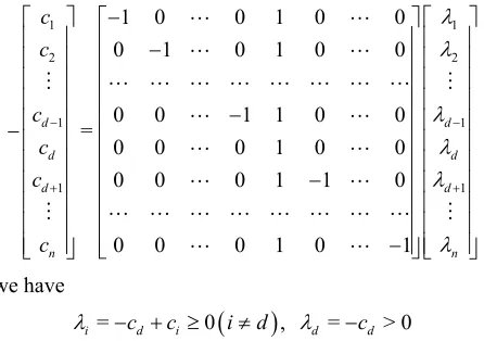
Executing the following simple procedure, we can readily find an initial ladder for the above problem. At start, take J = {m – n + 1, m – n + 2, ···, m – n + d, ···, m}. Let cd = max{ci} > 0 (1 ≤d ≤n). Take j = m – n + d
as a drop (the associated constraint is –xd≤bm – n + d) and
p = m + 1 a pick (the associated constraint is –x1 – x2 – ··· – xn≤M). It is easy to verify that J(j ↔p) is a
lad-der generator of the above problem. Indeed, from
1 1
2 2
1 1
1 1
1 0 0 1 0 0
0 1 0 1 0 0
0 0 1 1 0 0
=
0 0 0 1 0 0
0 0 0 1 1 0
0 0 0 1 0 1
d d d d d d n n c c c c c c we have
= 0 , =
i cd ci i d d cd
> 0
which implies J(j ↔p) is a ladder generator of the above problem.
3.2. Variables with Lower Bounds
In this subsection, we consider the case where variables of problem (P) have lower bounds. For convenience of discussion, we rewrite the problem in the following form: (P2) min c x1 1c x2 2 c xd d c xn n
11 1 12 2 1 1
s.t. a x a x a xn n b
21 1 22 2 2n n 2 a x a x a x b
m n1 1 m n2 2 m n n n m
a x a x a x b n
1 m n 1 x b
2 m n 2 x b
d m n
x b d
n m
x b
Note that here we use the same notations in problem (P2) as in (P1) for convenience. In this subsection, we temporarily assume that c contains at least one negative component. With this assumption, it is easy to be seen that the index set {m – n + 1, m – n + 2, ···, m – n + d, ···, m} is not a ladder generator. Adding an artificial con-straint
ni1xiMmin c x
, we get the following system:
1 1c x2 2 c xd d c xn n
11 1 12 2 1 1
s.t. a x a x a xn n b
21 1 22 2 2n n 2 a x a x a x b
m n1 1 m n2 2 m n n n m
a x a x a x b n
1 m n 1 x b
2 m n 2 x b
d m n
x b d
n m
x b
1 2 n
x x x M
1 Performing the similar procedure as the above subsection, we can easily obtain an initial ladder for the above problem. Initially, take J = {m – n + 1, m – n + 2, ···, m – n + d, ···, m}. Let cd = min{ci} < 0 (1 ≤d ≤n). Take j = m – n + d as
a drop (the associated constraint is –xd≤bm–n+d) and p = m
+ 1 as a pick (the associated constraint is x1 + x2 + ··· + xn≤
M). It is easy to verify that J(j ↔p) is a ladder generator of the above problem. In fact, from
1 1
2 2
1
1 1
1 0 0 1 0 0
0 1 0 1 0 0
0 0 1 1 0 0
=
0 0 0 1 0 0
0 0 0 1 1 0
0 0 0 1 0 1
d d d d d d n n c c c c c c > 0 3 we have
= 0 , =
i cd ci i d d cd
which implies J(j ↔p) is a ladder generator of the above problem.
If variables in an LP problem are bounded from both below and above, that is, an LP problem contains n con-straints taking the form of li≤ xi≤ui (1 ≤i ≤n), where li
and ui denote the lower and upper bounds of xi and li < ui,
then after rewriting the above constraints as two con-straints –xi≤−li and xi≤ui we can follow the procedure in
either Subsection 3.1 or Subsection 3.2 to obtain an ini-tial ladder for the problem.
4. A Specific Example
To illustrate the efficiency of the above ladder algorithm, we use both the simplex method and MCCA to solve a Klee-Minty problem [7,8].
Example 1 Consider the following Klee-Minty
prob-lem with n = 3
1 2
min 100 x 10x x
1 s.t. x 1
1 2 20x x 100
1 2 3
200x 20x x 10,000
1, , 0.2 3
x x x
On the one hand, we use the simplex method to solve the above problem. Introducing the slack variables s1, s2, s3 ≥ 0, write the above problem as the standard form
1 2
min 100 x 10x x3
1 1 s.t. x s = 1
1 2 2
20x x s = 100
1 2 3 3
200x 20x x s = 10,000
1, , , , , 02 3 1 2 3
x x x s s s
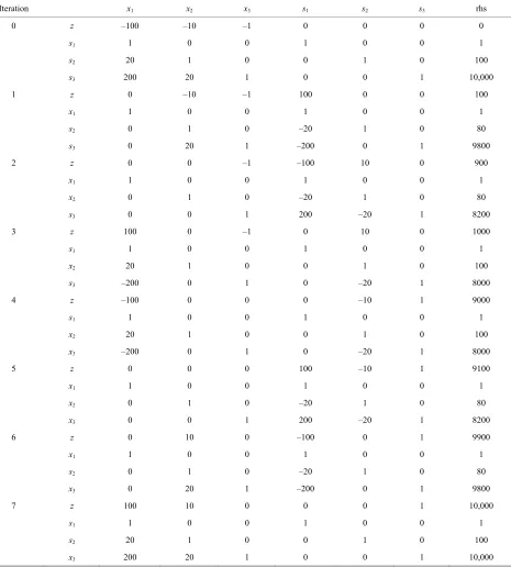
The tableau in Table 1 shows that the simplex method
with the most negative rule requires 2n – 1 = 23 – 1 = 7 iterations to attain the optimality.
On the other hand, we solve the same problem using MCCA. Firstly we rewrite all constraints as ≤–type:
1 2
min 100 x 10x x3
1 s.t. x 1
1 2 20x x 100
1 2 3
200x 20x x 10,000
1 0 x 2 0 x 3 0 x
To find an initial ladder, we add an artificial constraint x1 + x2 + x3 ≤ M. For clarity, write the problem with the additional constraint as below.
1 2
min 100 x 10x x3
1 s.t. x 1
1 2 20x x 100
1 2 3
200x 20x x 10000
1 0 x 2 0 x 3 0 x
1 2 3
x x x M
It is easy to verify that the index set {7, 5, 6} is an ini-tial ladder generator (see Subsection 3.2). With the known ladder generator at hand, it takes only two itera-tions to reach an optimal solution for MCCA. For solu-tion detail, see Table 2.
[image:4.595.60.283.289.446.2]Table 1. The tableau obtained from simplex for Example 1.
Iteration x1 x2 x3 s1 s2 s3 rhs
0 z –100 –10 –1 0 0 0 0
s1 1 0 0 1 0 0 1
s2 20 1 0 0 1 0 100
s3 200 20 1 0 0 1 10,000
1 z 0 –10 –1 100 0 0 100
x1 1 0 0 1 0 0 1
s2 0 1 0 –20 1 0 80
s3 0 20 1 –200 0 1 9800
2 z 0 0 –1 –100 10 0 900
x1 1 0 0 1 0 0 1
x2 0 1 0 –20 1 0 80
s3 0 0 1 200 –20 1 8200
3 z 100 0 –1 0 10 0 1000
s1 1 0 0 1 0 0 1
x2 20 1 0 0 1 0 100
s3 –200 0 1 0 –20 1 8000
4 z –100 0 0 0 –10 1 9000
s1 1 0 0 1 0 0 1
x2 20 1 0 0 1 0 100
x3 –200 0 1 0 –20 1 8000
5 z 0 0 0 100 –10 1 9100
x1 1 0 0 1 0 0 1
x2 0 1 0 –20 1 0 80
x3 0 0 1 200 –20 1 8200
6 z 0 10 0 –100 0 1 9900
x1 1 0 0 1 0 0 1
s2 0 1 0 –20 1 0 80
x3 0 20 1 –200 0 1 9800
7 z 100 10 0 0 0 1 10,000
s1 1 0 0 1 0 0 1
s2 20 1 0 0 1 0 100
x3 200 20 1 0 0 1 10,000
Table 2. The table obtained from MCCA for Example 1.
Iteration Ladder generator Base point Optimal value
0 {7,5,6} [M; 0; 0]
1 {7,5,3} 10,000 ; 0; 10,000 200
199 199
M M
[image:5.595.57.543.646.737.2]although here we use an example with non-negativity variables to illustrate the efficiency of our algorithm, there is no non-negativity requirement for variables in our problem form. Thus, our algorithm is suitable for a wider range of LP problems.
5. Numerical Tests
In this section, we make computational tests to demon-strate the efficiency of MCCA. The ladder algorithms were coded in MATLAB 7.11.0. Test problems are ran-domly generated in the same way as in [5], which is pre-sented as below.
Example 2 [5](Randomly generated feasible problem)
Generate a linear programming problem by specifying m n
A R , =
1; ; ;2
n n
c c c c R , and
1 2
1. Randomly generate and a vector = ;
b b b ; ; m
m
b R
n
c R
in the following method.
n
xR such that components of c take values between –25 and 25, and components of x between 0 and 20.
2. Generate A and b by two steps.
(a) For 1 ≤ j ≤ n, the j-th row aj of A is
= T 2sign
j j j
a c c e , where ej is the j-th row of the n ×
n identity matrix. Then, bj is defined by bj =a xj j,
where γj is a random number in (0, 1).
(b) For n + 1 ≤j≤m, randomly generate a row vector and a number j
n
j R
R such that βj and all the
components of αj are between –25 and 25. If jxj,
then the j-th row aj of A and the j-th element of b are
de-fined by aj = αj, bj = βj. Otherwise, they are defined by aj =
−αj, bj = −βj.
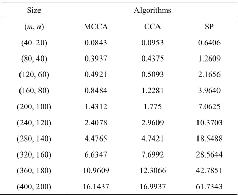
Tests were run on a desk-top computer (HP Intel(R) Core(TM), i7-2600 [email protected], 3.39GHz, 3.24GB of RAM) under Microsoft Windows XP operating system. For comparison, the centered climbing algorithm (CCA) [5] and the linprog solver in MATLAB optimization toolbox (Version 5.1, (R2010b)) were used for solving the same test problems. The medium-scale simplex algo-rithm (SP) was implemented. Tables 3 and 4 present
computational results for 20 test problems with various dimensions. The average CPU time is reported in sec-onds. Since our algorithm and the simplex method actu-ally work on problems with different forms and dimen-sions, the number of iterations does not provide much helpful information. Therefore, here we do not take the comparison of iteration numbers into account.
Tables 3 and 4 reveal that, MCCA has the absolute
[image:6.595.307.539.111.301.2]advantage over CCA as well as the simplex method for tested problems. We would like to point out that in the present code we adopt the traditional technique of the inverse of matrix to calculate base points. If the advanced numerical technique was incorporated into the current code, the computational performance would promise further improvement.
Table 3. Average CPU time (in seconds) for test problems in Example 2 (m = 2n).
Size Algorithms
(m, n) MCCA CCA SP
(40. 20) 0.0843 0.0953 0.6406
(80, 40) 0.3937 0.4375 1.2609
(120, 60) 0.4921 0.5093 2.1656
(160, 80) 0.8484 1.2281 3.9640
(200, 100) 1.4312 1.775 7.0625
(240, 120) 2.4078 2.9609 10.3703
(280, 140) 4.4765 4.7421 18.5488
(320, 160) 6.6347 7.6992 28.5644
(360, 180) 10.9609 12.3066 42.7851
[image:6.595.307.539.338.512.2](400, 200) 16.1437 16.9937 61.7343
Table 4. Average CPU time (in seconds) for test problems in Example 2 (m – n = 100).
Size Algorithms
(m, n) MCCA CCA SP
(600, 500) 35.8554 40.8424 126.6692
(650, 550) 44.75 57.9263 148.9732
(700, 600) 52.25 72.5273 185.5312
(750, 650) 62.2291 73.6718 225.5625
(800, 700) 75.7187 118.7760 239.6666
(850, 750) 97.3125 99.4531 240.1953
(900, 800) 94.9375 122.8281 252.8281
(950, 850) 112.5312 155.4531 280.9843
(1000, 900) 117.5937 147.9531 345.1093
6. Conclusion
A new ladder algorithm, termed “the Modified Centered Climbing Algorithm”, was proposed in this paper. Com-putational results demonstrated that the ladder algorithm outperforms CCA as well as the simplex algorithm in terms of average CPU time for randomly generated test problems. In addition, the single artificial constraint technique was presented to initialize the ladder method for LP problems with bounded variables. An illustration showed that this initialization technique is intuitive and simple.
REFERENCES
[1] G. B. Dantzig, “Linear Programming and Extensions,” Princeton University Press, Princeton, 1963.
Linear Programming,” Combinatorica, Vol. 4, No. 4, 1984, pp. 373-395. doi:10.1145/800057.808695
[3] K. G. Murty and Y. Fathi, “A Feasible Direction Method for Linear Programming,” Operations Research Letters, Vol. 3, No. 3, 1984, pp. 121-127.
doi:10.1016/0167-6377(84)90003-8
[4] L. G. Khachian, “A Polynomial Algorithm in Linear Pro- gramming,” Soviet Mathematics Doklady, Vol. 20, 1979, pp. 191-194.
[5] Y. Liu, “An Exterior Point Linear Programming Method Based on Inclusive Normal Cones,” Journal of Industrial
and Management Optimization, Vol. 6, No. 4, 2010, pp. 825-846. doi:10.3934/jimo.2010.6.825
[6] M.-F. Ding, Y. Liu and J. A. Gear, “An Improved Tar-geted Climbing Algorithm for Linear Programs,” Nu-merical Algebra, Control and Optimization (NACO), Vol. 1, No. 3, 2011, pp. 399-405. doi:10.3934/naco.2011.1.399
[7] R. J. Vanderbei, “Linear Programming: Foundations and Extensions,” 3rd Edition, Springer, New York, 2008. [8] V. Klee and G. J. Minty, “How Good Is the Simplex