Proportional Controller from Control Theory for Tuning cooling scheme of Simulated Annealing algorithm

Received May 24, 2016 / Accepted Sep 11, 2017

Editorial Académica Dragón Azteca (EDITADA.ORG)

Proportional Controller from Control Theory for Tuning cooling scheme

of Simulated Annealing algorithm

Eduardo Rodríguez del Angel

, Juan Frausto-Solis

, J. David Terán-Villanueva

, Héctor

Joaquín Fraire Huacuja

.

Tecnológico Nacional de México: Instituto Tecnológico de Ciudad Madero.

[email protected]

, [email protected]

, [email protected]

[email protected]

Abstract. To solve difficult problems of combinatorial optimization, heuristic methods such as Simulated Annealing (SA) and Threshold algorithm (TA) have been proposed. Both SA and TA should have adequate characteristics to explore efficiently the space of solutions. The process to determine these characteristics is known as parameter tuning problem. There is a strong interest in developing techniques to adjust parameters correctly, since the heuristic algorithms have a great applicability in industrial problems. Given the quantitative nature of multiple parameters it is possible to propose the selection of the best parameters of a heuristic as a combinatorial optimization problem. In this paper, a new tuning method based on the proportional controller derived from classical control theory for tuning the cooling scheme in real time is presented. Experimentation shows that this method has a better performance than the classical one.

Keywords: Parameter Tuning, heuristic algorithms, Control Theory. Simulated Annealing, Threshold algorithm.

1.

Introduction

To solve combinatorial optimization problems, which present a large space of solutions, heuristic methods have been developed that seek to effectively explore this space to find solutions of good quality in an acceptable time. For the execution of a heuristic method it is necessary to select within many possibilities a series of features known as parameters that defines the behavior of the algorithm, that process is known as parameter tuning.

In general, the problem of parameter tuning consists in the selection of a parameter configuration that generates quality solutions [1]. The parameters are classified in: a) Qualitative parameters, that select methods or functions that will be executed in the algorithm, b) Quantitative parameters, which define aspects of the operation of the algorithm, which are usually numerical.

The good or bad execution of heuristic algorithms is based on the appropriate selection of the parameters with which the algorithm works. The parameter tuning is applied in two ways:

1. Off-line, when the execution of the algorithm must be stopped to modify the values of the parameters, these changes will not be reflected until the next execution of the algorithm.

2. Online, when the execution does not stop to modify them. The advantage of the latter is that the changes will be reflected during the next iteration of the algorithm.

17

Classical control techniques such as proportional, integral and derivative control have been shown to obtain good results by controlling industrial processes that are subject to constant changes by monitoring the state of the output and modifying the behavior of the process during its execution. The objective of this work is to implement the proportional control technique to modify the behavior of the Simulated Annealing algorithm (SA).

A method was developed that modifies the cooling scheme depending on the quality of the solutions taking inspiration in the proportional control. This method was incorporated to the method of analytical tuning [2] and the experimentation was carried out comparing the performance of 3 types of tunings: manual, analytical and the proposal in this work.

Section 2 describes concepts derived from traditional control theory in order to reinforce the analogy between an industrial process that can be monitored in real time and the algorithm. Section 3 describes the Simulated Annealing and Threshold algorithms, including a general description of their operation and their parameters.

In addition, this section includes the description of an off-line tuning method called "analytical tuning" and the description of the proposed new method. The analytical tuning will serve to generate an initial configuration of the parameters and the cooling scheme will be modified using the proportional operator. Sections 4 and 5 describe the tests performed and the conclusions obtained in this work.

2.

Control theory operators

A system can be defined as a black box where its input and output is known, but the content does not interest, but the interest lies in the relationship between the initial state and the final state, as shown in Figure 1. In an industrial process the input is defined as all the raw materials and initial conditions that the process receives and that will be converted through a series of steps (system) in an output, what defines the behavior of the system is specified in the set point. The systems can be open or close loop.

Figure 1. System as a black box.

An open loop system is shown on Figure 2; in this case, the output has no effect on the control action [3]. In an open loop system, the output information of a process does not feed back into the system, which does not allow to know if the result obtained is close to the desired result. The disadvantage of this type of systems is that any modification to the behavior of the system will generate a malfunction and due to the lack of information of the output it is not possible to make corrections.

Figure 2. Open loop system.

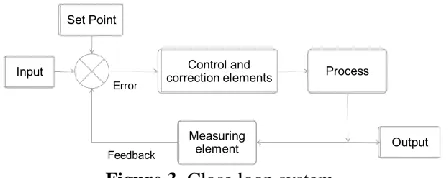
In closed loop systems, the output feeds back to the controller, Figure 3, in order to reduce the error that may exist [4]. Because the state of the variables is known during the process, it is possible to generate a system that is modified during its execution, creating an automatic control system. An advantage of this system is that feedback allows the system to adapt to external disturbances. The feedback can be exploited by a controller.

18

Currently, in industrial processes, different control strategies have been implemented to try to regulate and manipulate the operating conditions of these processes, one of the strategies that has been implemented with greater success due to its low complexity, relatively low cost and adaptability is the proportional controller. In the proportional controller, the correction signal increases as the error occurs, producing large changes in the final control element in cases where the deviation is greater and small changes otherwise.

3.

Simulated Annealing and Threshold algorithm

The simulated annealing (SA) algorithm is a heuristic algorithm proposed by Kirkpatrick [5] whose operation is based on the analogy that can be found between a combinatorial optimization process and the thermodynamic process of metal annealing. Besides, Threshold Algorithm (TA) is too similar to SA, the only difference is the acceptance criteria [6]. As is shown in Algorithm 1, SA and TA are in fact very simple algorithms with only two loops.

The external cycle is a cycle of temperatures which is repeated since the initial to the final temperature. The internal loop is known as the metropolis cycle and at each iteration of the Metropolis cycle an important function called perturbation function (or perturbation in short) is executed. This function takes the current solution 𝑆𝑖 and generates a neighbor solution 𝑆𝑗 for which

the objective function value 𝐸(𝑆_𝑗) is calculated. The difference between 𝐸(𝑆_𝑗) and the current objective function value 𝐸(𝑆_𝑖) is

then calculated as ∆ (see equation 1). An acceptance function is then used to decide if the new solution is better than the current one; this is done to decide whether to accept or not the new solution.

Algorithm 1. Simulated Annealing algorithm and Threshold algorithm.

1. 𝑆𝐴 𝑎𝑛𝑑 𝑇𝐴 𝑎𝑙𝑔𝑜𝑟𝑖𝑡ℎ𝑚𝑠(𝛼, 𝛽, 𝑛, 𝑇𝑜, 𝑇𝑓, 𝐿𝑜, 𝐿𝑓, 𝑇ℎ) {

2. 𝑇𝑐𝑢𝑟𝑟𝑒𝑛𝑡= 𝑇𝑜;

3. 𝑆𝑖= 𝑔𝑒𝑛𝑒𝑟𝑎𝑡𝑒𝐼𝑛𝑖𝑡𝑖𝑎𝑙𝑆𝑜𝑙𝑢𝑡𝑖𝑜𝑛();

4. 𝒘𝒉𝒊𝒍𝒆 𝑇𝑐𝑢𝑟𝑟𝑒𝑛𝑡 ≥ 𝑇𝑓 || 𝑜𝑝𝑡𝑖𝑚𝑎𝑙𝐹𝑜𝑢𝑛𝑑() 𝒅𝒐 {

//𝑬𝒙𝒕𝒆𝒓𝒏𝒂𝒍 𝒕𝒆𝒎𝒑𝒆𝒓𝒂𝒕𝒖𝒓𝒆 𝒄𝒚𝒄𝒍𝒆

5. 𝒘𝒉𝒊𝒍𝒆 𝑚𝑒𝑡𝑟𝑜𝑝𝑜𝑙𝑖𝑠(𝛽) 𝒅𝒐 {

//𝑰𝒏𝒕𝒆𝒓𝒏𝒂𝒍 𝑴𝒆𝒕𝒓𝒐𝒑𝒐𝒍𝒊𝒔 𝒄𝒚𝒄𝒍𝒆

6. 𝑆𝑗= 𝑔𝑒𝑛𝑒𝑟𝑎𝑡𝑒𝑁𝑒𝑖𝑔ℎ𝑏𝑜𝑟(𝑆𝑖);

7. ∆ = 𝐸(𝑆_𝑗)− 𝐸(𝑆_𝑖);

8. 𝒂𝒄𝒄𝒆𝒑𝒕𝒂𝒏𝒄𝒆𝑭𝒖𝒏𝒄𝒕𝒊𝒐𝒏(∆);

9. 𝑢𝑝𝑑𝑎𝑡𝑒𝑆𝑜𝑙𝑢𝑡𝑖𝑜𝑛(𝑆𝑗);

} 𝒆𝒏𝒅𝒘𝒉𝒊𝒍𝒆

10. 𝑢𝑝𝑑𝑎𝑡𝑒𝑃𝑎𝑟𝑎𝑚𝑒𝑡𝑒𝑟𝑠(𝛼, 𝛽, 𝑇𝑐𝑢𝑟𝑟𝑒𝑛𝑡, 𝐿𝑐𝑢𝑟𝑟𝑒𝑛𝑡);

} 𝒆𝒏𝒅𝒘𝒉𝒊𝒍𝒆 }

Equation (1) is used in the acceptance criterion as follows. A new solution is accepted if: 1) the new solution improves the previous one; 2) If the new solution worsens, but meets the acceptance criteria, the new solution is accepted, even if the quality of the solution is not better than the current solution. Among the acceptance criteria used are Boltzmann's criterion and Threshold’s criterion, both explained later. In fact, the only difference between SA and TA algorithms are the acceptance criteria.

∆ = 𝐸(𝑆𝑗)− 𝐸(𝑆𝑖) . (1)

19

𝑒−∆⁄𝑇𝑐𝑢𝑟𝑟𝑒𝑛𝑡> 𝑟𝑎𝑛𝑑𝑜𝑚(0, 1) _. (2)

Threshold criteria: Every solution with a lower cost than the current solution is accepted. However, a threshold parameter allows to accept a certain fraction of bad solutions, without to perform calculations of exponentials or use functions that generate random numbers, which are costly for programs [6].

3.1 Algorithms parameters

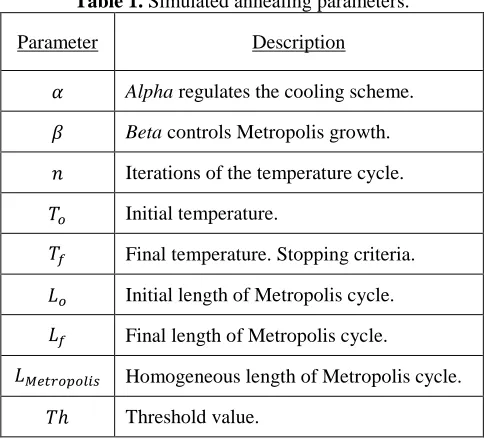
SA and TA as many other heuristics have a certain number of parameters which should be tuned to have an adequate algorithm. Table 1 shows the parameters commonly used in both algorithms.

Table 1. Simulated annealing parameters.

Parameter Description

𝛼 Alpha regulates the cooling scheme. 𝛽 Beta controls Metropolis growth. 𝑛 Iterations of the temperature cycle. 𝑇𝑜 Initial temperature.

𝑇𝑓 Final temperature. Stopping criteria.

𝐿𝑜 Initial length of Metropolis cycle.

𝐿𝑓 Final length of Metropolis cycle.

𝐿𝑀𝑒𝑡𝑟𝑜𝑝𝑜𝑙𝑖𝑠 Homogeneous length of Metropolis cycle.

𝑇ℎ Threshold value.

Length of the Metropolis cycle: The internal cycle is repeated depending on the length proposed, the two main trends to delimit the length are the following:

a) Homogeneous length: For all temperatures, the cycles will have the same length (𝐿𝑀𝑒𝑡𝑟𝑜𝑝𝑜𝑙𝑖𝑠).

b) Non-Homogeneous length: It is proposed in [7] and [8] that the length of the cycles at high temperatures is less than the length at high temperatures, as shown in equation (3). At high temperatures, the acceptance criterion allows to accept many solutions which generates a lot of diversity; in contrast at low temperatures the criterion is more restrictive which causes that generally only to accept solutions that improve the previous one.

As a consequence, for the metropolis cycle a geometrical length is proposed [7].

𝐿𝑘+1= 𝛽 ∗ 𝐿𝑘 . (3)

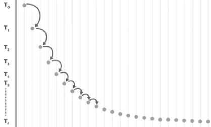
Cooling scheme: The SA starts at a high initial temperature 𝑇0 and at each iteration of the external cycle decreases until reaching a final stop temperature 𝑇𝑓, based on the selected cooling scheme. Table 2 shows different cooling schemes.

Table 2. Different cooling schemes.

Schema type Recurrence relation

Geometrical 𝑇𝑘+1= 𝛼 ∗ 𝑇𝑘

Exponential 𝑇𝑘+1= 𝑇𝑘∗ 𝑒−𝛼

20

When using the geometrical cooling scheme, the alpha value must be a percentage less than 100% and to perform a slow cooling, it is suggested in [9] that alpha be selected from the interval given in equation (4).

0.8 ≤ 𝛼 ≤ 0.9 . (4)

Figure 4 shows a graphical representation of how the temperature changes through the different repetitions of the external cycle of the algorithm.

Figure 4. Curve of temperatures obtained with the geometrical cooling scheme.

3.2 Analytical tuning

The analytical tuning technique proposed in [2] and [7] consists of the analysis of the geometrical cooling scheme and the linear equation that is found when using a non-homogeneous Metropolis cycle, in order to obtain the parameter value through mathematical relations. The initial and final temperatures are defined using Boltzmann criteria, equation (5), as the probability of accepting a solution. Such that:

𝑃𝑎= 𝑒 −∆

𝑇

⁄ _{. (5)}

Solving for the temperature of the equation (5) we obtain equation (6).

𝑇 = −∆ ln 𝑃⁄ 𝑎 . (6)

For high temperatures, near the initial temperature 𝑇𝑜, the acceptance criterion is more permissive, because the probability of

acceptance is high 𝑃ℎ𝑖𝑔ℎ; on other hand for low temperatures, near the final temperature 𝑇𝑓, the criterion is more restrictive, even

for very close solutions, given the fact that the probability of acceptance is low 𝑃𝑙𝑜𝑤.

𝑇𝑜= −∆𝑀𝑎𝑥 ln 𝑃⁄ ℎ𝑖𝑔ℎ . (7)

𝑇𝑓= −∆𝑀𝑖𝑛 ln 𝑃⁄ 𝑙𝑜𝑤 . (8)

The maximum and minimum energy delta are variables that depend on the problem to be solved generally associated with the objective function, while the acceptance probabilities 𝑃ℎ𝑖𝑔ℎand 𝑃𝑙𝑜𝑤 are very close to one or very close to zero respectively, and

are chosen by the user, in the suggested ranges, equations (9) and (10):

0.90 ≤ 𝑃ℎ𝑖𝑔ℎ ≤ 0.99 . (9)

0.01 ≤ 𝑃𝑙𝑜𝑤 ≤ 0.1 . (10)

The geometrical cooling scheme, equation (11) allow us to find the value of “n”, by solving given equation as seen on equation

(12), which represents the total of cycles of different temperatures between the initial temperature and the final temperature.

𝑇𝑓 = 𝛼𝑛 𝑇0 . (11)

𝑛 =ln 𝑇𝑓−ln 𝑇0

ln 𝛼 .

21

In the work of [7] it is proposed that the length of the Metropolis cycles at high temperatures is less than the length at high temperatures, to avoid diversification. And it relates the final length 𝐿𝑓 of the cycle to the solution space to be explored, so that

by using the linear growth function for non-homogeneous cycles, equation (13) it is possible to find the value of the beta parameter equation (14).

𝐿𝑓 = 𝛽𝑛∗ 𝐿0 . (13)

𝛽 = 𝑒ln 𝐿𝑓−ln 𝐿0𝑛 . (14)

3.3 Tuning using control theory

A cooling technique is proposed which modifies the alpha during the execution of the algorithm so that, if the solution improves to the solution of the previous temperature cycle, alpha is reduced in order that the stop condition is reached before and perform less cycles that may impair the quality of the current solution, but in case the solution does not improve or remain the same the original alpha parameter is handled (Algorithm 2).

Algorithm 2.

Modified temperature cycle.

𝒘𝒉𝒊𝒍𝒆 𝑇𝑐𝑢𝑟𝑟𝑒𝑛𝑡 ≥ 𝑇𝑓 𝑜𝑝𝑡𝑖𝑚𝑎𝑙𝐹𝑜𝑢𝑛𝑑() 𝒅𝒐 {

1 𝑞𝑢𝑎𝑙𝑖𝑡𝑦𝑝𝑟𝑒𝑣𝑖𝑜𝑢𝑠= 𝑒𝑣𝑎𝑙𝑢𝑎𝑡𝑖𝑜𝑛(𝑆𝑖);

2 𝑆𝑖= 𝑚𝑒𝑡𝑟𝑜𝑝𝑜𝑙𝑖𝑠𝐶𝑦𝑐𝑙𝑒(𝑆𝑖)

3 𝑞𝑢𝑎𝑙𝑖𝑡𝑦𝑛𝑒𝑤= 𝑒𝑣𝑎𝑙𝑢𝑎𝑡𝑖𝑜𝑛(𝑆𝑖);

𝒊𝒇 (𝑞𝑢𝑎𝑙𝑖𝑡𝑦𝑛𝑒𝑤 < 𝑞𝑢𝑎𝑙𝑖𝑡𝑦𝑝𝑟𝑒𝑣𝑖𝑜𝑢𝑠)

4 𝛼𝑝𝑟𝑜𝑝𝑜𝑟𝑡𝑖𝑜𝑛𝑎𝑙 = 𝑢𝑝𝑑𝑎𝑡𝑒𝐴𝑙𝑝ℎ𝑎( );

5 𝑢𝑝𝑑𝑎𝑡𝑒𝑃𝑎𝑟(𝛼𝑝𝑟𝑜𝑝𝑜𝑟𝑡𝑖𝑜𝑛𝑎𝑙, 𝛽, 𝑇𝑐𝑢𝑟𝑟𝑒𝑛𝑡, 𝐿𝑐𝑢𝑟𝑟𝑒𝑛𝑡);

𝒆𝒍𝒔𝒆

6 𝑢𝑝𝑑𝑎𝑡𝑒𝑃𝑎𝑟(𝛼, 𝛽, 𝑇𝑐𝑢𝑟𝑟𝑒𝑛𝑡, 𝐿𝑐𝑢𝑟𝑟𝑒𝑛𝑡);

} 𝒆𝒏𝒅𝒘𝒉𝒊𝒍𝒆

The 𝛼𝑝𝑟𝑜𝑝𝑜𝑟𝑡𝑖𝑜𝑛𝑎𝑙 parameter must be within the range defined in equations (15) and (16).

𝛼𝑚𝑖𝑛≤ 𝛼𝑝𝑟𝑜𝑝𝑜𝑟𝑡𝑖𝑜𝑛𝑎𝑙≤ 𝛼𝑚𝑎𝑥 . (15)

∆𝛼= 𝛼𝑚𝑎𝑥− 𝛼𝑚𝑖𝑛 . (16)

To calculate this, the equation (17) is proposed.

𝛼𝑝𝑟𝑜𝑝𝑜𝑟𝑡𝑖𝑜𝑛𝑎𝑙= 𝛼𝑚𝑖𝑛+ ∆𝛼∗ 𝑝𝑟𝑜𝑝𝑜𝑟𝑡𝑖𝑜𝑛𝑎𝑙𝐸𝑟𝑟𝑜𝑟 . (17)

Where the proportional error is in function to what is sought to solve in the instance and the value of the quality of the solution after the cycle of metropolis equation (18).

𝛼𝑝𝑟𝑜𝑝𝑜𝑟𝑡𝑖𝑜𝑛𝑎𝑙 = 𝛼𝑚𝑖𝑛+ ∆𝛼∗

𝑞𝑢𝑎𝑙𝑖𝑡𝑦𝑛𝑒𝑤

𝑜𝑏𝑗𝑒𝑐𝑡𝑖𝑣𝑒𝐹𝑢𝑛𝑐𝑡𝑖𝑜𝑛 . (18)

22

Figure 5. Curve of temperatures obtained with the modified cooling scheme.

4.

Experimentation and results

The quality of the solution was measured with the average percentage of clauses satisfied, also measuring the execution time of the three algorithms. The instances used were taken from the collection of instances SATLIB of the problem 3-SAT, the instances uf20-01 to uf20-020 were grouped in the set uf20; Uf50-01 to uf50-020 in the uf50 set; Instances uf75-01 to uf75-020 in the uf75 set, and then instances uf250-01 to uf250-040 in the uf250 set.

Each of the one hundred instances was solved 30 times by each algorithm and the results are shown in the following table. The average percentage of satisfied clauses obtained by each algorithm is shown in Table 3:

 A1: SA with manually defined parameters (𝛼 = 0.96, 𝑇0= 500, 𝑇𝑓= 0.01 and 𝐿𝑀𝑒𝑡𝑟𝑜𝑝𝑜𝑙𝑖𝑠= 50).

 A2: SA with parameters obtained by analytical tuning.

 A3: SA with parameters obtained by analytical tuning and the modified cooling scheme using the proportional operator.

Version B of the algorithms uses Boltzmann acceptance criterion while version T uses Threshold criterion.

Table 3. Results.

Instances Variables Clauses

Manually defined parameters

Analytical tuning No proportional

operator

Proportional operator

A1B A1T A2B A2T A3B A3T

Set uf20 20 91 99.80 91.58 99.87 99.55 99.68 99.58

Set uf50 50 218 98.48 87.95 99.74 99.60 99.54 99.48

Set uf75 75 325 97.82 87.52 99.77 99.64 99.55 99.53

Set uf250 250 1065 94.87 87.47 99.81 99.77 99.45 93.78

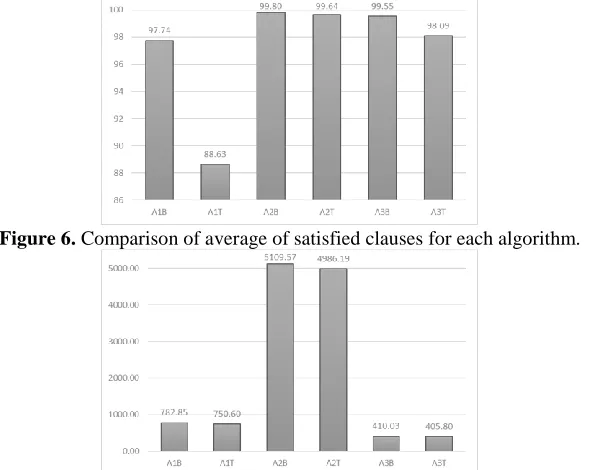
Great average of satisfied clauses 97.74 88.63 99.80 99.64 99.55 98.09

Running time (seconds) 782.85 750.60 5109.57 4986.19 410.03 405.80

% of improvement in quality against A1 - - 2.11 12.42 1.85 10.67 % of time improvement against A1 - - -552.69 -564.29 47.62 45.94

When comparing the algorithms A2 and A1 it is observed that the use of the analytical tuning of parameters produces an improvement in the quality of the solution at the cost of an increase in execution time close to 550% of the original value for both versions of the algorithms (Boltzmann and Threshold).

23

execution time to 45% of the original time in both Versions of the algorithms. This indicates that using the proportional controller is a superior alternative to the traditional analytical tuning technique, the use of other control theory techniques could improve the obtained results.

Figure 6. Comparison of average of satisfied clauses for each algorithm.

Figure 7. Comparison of running time (seconds) for each algorithm.

The obtained results (shown in Figure 6 and Figure 7) finds that the acceptance criterion of Threshold obtains better times, but a slightly smaller quality independent of the way in which the parameters were tuned with respect to the criterion of acceptance of Boltzmann, which is because it is a more permissive acceptance criterion, giving rise to the possibility of selecting more solutions that worsen the current one. The experimentation was carried out on a computer with a processor AMD Phenom 2 3.20 GHZ, 8 GB de RAM, Windows 7 service pack 7.

5.

Conclusions

In this paper, we present an on - line tuning method of the simulated annealing algorithm using the proportional control technique. Two variants of the annealing algorithm simulated with this technique were developed, one using the Boltzmann distribution as acceptance criterion and the other using the Threshold acceptance technique. The results show that the parameter tuning techniques obtained better results than the tests where the parameters were fixed, because they take information from the problem and modify its parameters with respect to the number of variables and clauses that the instance has.

Traditional control theory techniques have worked well in industrial processes by modeling any process as a plant to be monitored. It is observed that using the same work approach, presenting the algorithm as a plant to be controlled, obtains good results which invites to try other techniques of control theory for the management of parameters of a heuristic algorithm.

Acknowledgments

24

References

1. Birattari M. & Kacprzyk J.: Tuning metaheuristics: a machine learning perspective. Springer 197 (2009)

2. Frausto-Solis J., F. Alonso-Pecina, and C. Gonzalez-Segura: Analytically tuned parameters of simulated annealing for the Timetabling problem. Cimmacs ’07 Proc. 6th Wseas Int. Conf. Comput. Intell. Man-Machine Syst. Cybern. 5(5), 18–23 (2007)

3. Kuo B. C.: Digital control systems. Oxford University Press, Inc. (2007) 4. Ogata Katsuhiko: Modern Control Engineering. Pearson Prentice Hall (2010)

5. Kirkpatrick S., Vecchi M. P., & others: Optimization by simulated annealing. Science (80-.) 220 (4598), 671–680 (1983)

6. Dueck G. & Scheurer T.: Threshold Accepting: A General-Purpose Optimization Algorithm. J. Comput. Phys. 90, 161–175 (1990) 7. Frausto-Solís J., Sanvicente-Sánchez H., & Imperial-Valenzuela F.: ANDYMARK: an analytical method to establish dynamically the

length of the markov chain in simulated annealing for the satisfiability problem. Simulated Evol. Learn, 269–276 (2006).

8. Frausto-Solis J., Sánchez-Hernández J. P., Sánchez-Pérez M., & García E. L.: Golden Ratio Simulated Annealing for Protein Folding Problem. Int. J. Softw. Eng. Knowl. Eng. 12 (6), 1–20 (2013).