the case of some acoustic waves
Paul Kinsler∗Physics Department, Lancaster University, Lancaster LA1 4YB, United Kingdom. and
Blackett Laboratory, Imperial College London, Prince Consort Road, London SW7 2AZ, United Kingdom. (Dated: Friday 5th January, 2018)
The evolution of acoustic waves can be evaluated in two ways: either as a temporal, or a spatial propagation. Propagating in space provides the considerable advantage of being able to handle dispersion and propagation across interfaces with remarkable efficiency; but propagating in time is more physical and gives correctly behaved reflections and scattering without effort. Which should be chosen in a given situation, and what compromises might have to be made? Here the natural behaviors of each choice of propagation are compared and contrasted for an ordinary second order wave equation, the time-dependent diffusion wave equation, an elastic rod wave equation, and the Stokes’/ van Wijngaarden’s equations, each case illuminating a characteristic feature of the technique. Either choice of propagation axis enables a partitioning the wave equation that gives rise to a directional factorization based on a natural “reference” dispersion relation. The resulting exact coupled bidirectional equations then reduce to a single unidirectional first-order wave equation using a simple “slow evolution” assumption that minimizes effect of subsequent approximations, while allowing a direct term-to-term comparison between exact and approximate theories.
I. INTRODUCTION
An important category of acoustic wave models con-sists of those based on second order wave equations. Be-cause they include second order derivatives in both time and space, they naturally lend themselves to rearrange-ments designed to focus either on the temporal or the spa-tial behaviour. In practice, most acoustic wave models have more than just this pair of second order terms, and these extra contributions may (or may not) be suited to a preference for either temporal or spatial analysis. But despite the wide range of different acoustic wave models, a subset of cases is sufficient to cover most important modifications. Here we choose the time-dependent diffu-sion equation (TDDE) [1], a model for waves in an elas-tic cylindrical rod [2], and acouselas-tic waves as described by a generalized Stokes’ equation [3] which allows for bubbles [4]. For these three situations, harmonic solu-tions are well known, but transient solusolu-tions are harder to find. Recently, the impulse-response and causal prop-erties of some of these wave equations have been analyzed by Buckingham [5], and the (perhaps surprising) “non-causal” claims made therein are briefly addressed.
An advantage of second order wave equations is that once a propagation type is selected – whether into the future (i.e. along time), or along an appropriate spatial axis – they can be decomposed into pairs of explicitly directional andfirst order acoustic wave equations. The resulting coupled first order equations are not only of-ten easier and faster to solve than the starting point of a second order wave equation, they are also well suited to the case of unidirectional traveling waves. However the unidirectional approximation is not demanded, and the
∗Electronic address: [email protected]
formulation means that any additional approximations tend to be less restrictive [6]. For the purposes of this article, however, these desirable features are not the core message. Instead, by comparing the results of factoriza-tions aimed at generating temporally propagated wave equations, with those that generatespatially propagated ones, comparisons and contrasts can be made between the natural “reference” behaviors present in each decom-position.
A feature of the factorization approach is that it forces us to play close attention to the propagation axis, and to the distinctions between temporal and spatial choices [8]; the main differences being highlighted on fig. 1. How-ever, beyond the basic conceptual differences, an addi-tional aspect highlighted here is that for some wave mod-els, the temporal and spatial reference behaviours can be very different. We will see that some terms in a wave equation can lend themselves to inclusion in one reference behaviour but not the other. These results then inform us as to how we might choose to trade off the practical efficiency of a spatially propagated picture against the physically accurate temporally propagated one.
Section II provides an overview of the factorization pro-cess for both spatial and temporal decompositions, using the time domain diffusion equation as an example. Fac-torization is then used to analyze the TDDE in section III, acoustic waves in an elastic cylindrical rod in section IV, and the Stokes’ equation and its bubbly generaliza-tion in secgeneraliza-tion V. This variety allows a discussion of both common and contrasting features of these directional de-compositions. The conclusions are given in section VI.
II. DIRECTIONAL DECOMPOSITIONS
fac-torization technique. This makes use of the concept of “reference” or “underlying” wave evolution [6, 7]. If these reference behaviors are a close match to the ac-tual wave evolution, subsequent approximations will be less stringent – in particular if we choose to make a uni-directional approximation. Although in some systems an exact match is possible, this is rarely the case if the waves depart from some idealized linear behaviour. Nev-ertheless, the power of these directional decompositions is in considering such variation from these exactly solvable cases, situations which often require approximation or numerical integration. To “factorize”, start by selecting a propagation axis – either time, or along some spatial trajectory – after which the total wave can be decom-posed into directional components that evolve forwards or backwards perpendicular to that propagation. A more general discussion of the choices and interpretations pos-sible when choosing a propagation axis is given in [8].
Throughout this article the context and/or arguments determine which domains (~r or ~k, t or ω) a given in-stance of some relevant function covers; in addition some symbols (e.g. Q, Ω, κ, c, cΩ, cκ, etc) are reused
in-dependently of each other (for different wave equation models) without distinguishing subscripts – this is in or-der to avoid cluttering the notation. Further, each equa-tion for the relevant wave field g(~r, t) has, on the right hand side (RHS), a term Q which represents some gen-eral source term. Typically [5, 9] Q is an impulse de-signed to elicit the primitive response of the system (i.e.
Q=Qδ(t)δ(x)), but here it is allowed to be any kind of perturbation, (non)linear modification, or driving term we desire. For example, in the simple wave equations considered in this section, a dependence on the density
ρ(~r) could be added, settingQ = (1/ρ)∇ρ· ∇g, and so match a wave equation used for ultrasound propagation [10, 11]. Alternatively, adding a loss term to Q with the form η∂tg would give us the time-dependent diffu-sion equation (TDDE) [1], which appears in a variety of contexts in physics, including acoustic waves in plas-mas or the interstitial gas filling a porous, statistically isotropic, perfectly rigid solid [12]; it also models elec-tromagnetic wave propagation through conductive media and is known as the telegrapher’s equation.
In this section, an ordinary second order wave equa-tion for some appropriate wave propertyg(~r, t) (typically a velocity potential, or a displacement) will be used as a test bed on which to demonstrate the factorization pro-cess. It contains both a temporal response functionp(t) and a spatial one s(~r), both have a non-local charac-ter which is allowed for using a convolution (“?”), with
a(u)? b(u)≡R
a(u0)b(u−u0)du0. Whilst some materials, in some regimes, do indeed have non-local spatial prop-erties, the role of s(~r) here is to ensure that the wave equation includes some nontrivial spatial properties. In many situations spatial structure would be introduced using p(~r, t) instead of just p(t), while s(~r) and its con-volution would be absent; however here that would in-troduce complications beyond the scope of this example.
The wave equation is
c2∇2s(~r)? g(~r, t)−∂2
tp(t)? g(~r, t) =c
2Q(x, t), (2.1)
where a non-interacting wave travels with speedc. Upon Fourier transforming into thek, ωdomain, whered/dt≡ ∂t↔ −ıωand∇ ↔+ı~k, withk2=~k·~k, the result is
c2k2s(~k)g(k, ω)−ω2p(ω)g(~k, ω) =−c2Q(~k, ω), (2.2)
where s(~k) is the spatial Fourier transform ofs(~r), and
p(ω) the temporal Fourier transform ofp(t).
In both styles of derivation that follow, the steps taken are a good mathematical match to typical spatial propa-gation procedures [6, 13]; but the physical meaning alters with the interchange of the roles of time and space. Fac-torization methods have a long history [14], but their adaption, application, and adoption to wave propagation of the type and context proposed here has been lacking until more recently [15–17].
SinceQcan contain any sort of behaviour, eqn. (2.2) is already useful: e.g. factorization could easily be applied to the nonlinear propagation addressed by Pinton et al. [18]. In that case their initial eq. (3) can be matched to eqn. (2.1) above by restricting to the x-axis, using
c2s(x) = µδ(x), p(t) = ρδ(t), and setting Q to match
their RHS nonlinear term. Using directional decomposi-tion, a first order wave equation simpler than e.g. eq.(10) in Pinton et al. can be obtained rapidly with fewer and less restrictive approximations. Of course, some acous-tic wave equations reduced down to apply to a single wave property will not have the second order derivatives needed for this factorization scheme. However, such wave equations are already extensively approximated, so there may be scope for factorizing related equations which do contain them.
A. Temporal propagation, spatial decomposition
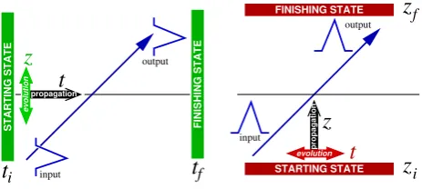
The most physically motivated factorization is to choose topropagate forward in time, and decompose the system behaviour (waves) into directional components that then evolve either forward or backward in space, as shown in Fig. 1. This is useful for analyzing situa-tions where signals need to be separated from reflecsitua-tions, but requires an explicit modeling of the medium’s time-response, perhaps involving convolutions or auxiliary dif-ferential equations.
To obtain such a temporally propagated, spatially de-composed representation, choose a suitable reference fre-quency Ω. This is allowed to have a wavevector (k) de-pendence, but should not have a frequency (ω) depen-dence. Rewriting eqn. (2.2) for temporal propagation,
¯
Ω(~k, ω)2g(~k, ω)−ω2g(~k, ω) =− c
2
p(ω)Q(
input
output
f
t
i
t
z
t
evolution
propagation
STARTING STATE FINISHING STATE
z
t
outputinput
propagation
evolution
z
iz
fFINISHING STATE
[image:3.595.59.291.55.159.2]STARTING STATE
FIG. 1: For temporal propagation (left), initial conditions cover all space at an initial timeti; the final state attf also covers all space. For spatial propagation (right), what are normally considered to be boundary conditions take up the role of the initial conditions; at both the starting locationxi and the final location ofxf, they specify the wave’s behaviour over all time. In theunidirectional case, only forward-going wave evolution is treated, so that any reflections – whether from defined interfaces or other changes in the material prop-erties – are neglected. Figures adapted with permission from [8].
with ¯Ω(~k, ω)2 =c2k2s(~k)/p(ω). Unfortunately, the
fre-quency dependence of ¯Ω means that it is not a good ref-erence on which to decompose the propagation. Thus we must either ignore the material’s frequency response
p(ω), treat it as a correction by incorporating it into Q, or convert its frequency response into a wavevector re-sponsep(k) by approximation1.
If there is no temporal response, then p(t) ≡ p0δ(t)
andp(ω) =p0, and the wave equation becomes
Ω(k)2g(~k, ω)−ω2g(~k, ω) =−c2Q(~k, ω)/p0, (2.4)
with Ω(~k)2 = c2k2s(~k)2/p
0. Eqn. (2.4) can be
rear-ranged to give an expression forg(~k, ω) directly, i.e.
g= c
2
ω2−Ω2
Q p0
=− 1
2Ω
1
ω+ Ω− 1
ω−Ω
c2Q
p0
,
(2.5)
Now decompose g into wave components g+ and g− that evolve either forward or backward in space, with
g=g++g−. Then split eqn. (2.5) into two coupled first order wave equations forg±(~k, t), i.e.
g±=± 1 2Ω
1
ω∓Ω
c2Q
p0
(2.6)
[ω∓Ω]g±=± 1 2Ω
c2Q
p0
, (2.7)
1 For example, if restricted to waves near a frequency ω 1 in a
narrow bandwidth ∆ω ω1, we can write ω ' c0k, where c0=ω
1/k, and replacep(ω) withs(k) – i.e. convert a temporal
dispersion into an approximate spatial dispersion. This is what was assumed in [19], and has been discussed at greater length in [20].
leading to either frequency or time domain forms
ωg±(~k, ω) =±Ω(k)g±(~k, ω)± 1 2Ω(~k)
c2Q(k, ω)
p0
, (2.8)
∂tg±(~k, t) =∓ıΩ(~k)g±(~k, t)∓
ı
2Ω(~k)
c2Q(~k, t) p0
. (2.9)
This last equation tells us how g±(~k, t) evolves [or if appropriately transformed, g±(~r, t)] as we propagate in time. The original second order equation can be recovered[13] by substituting one of these into the other. Note that retaining a frequency dependence for Ω would have given rise to time derivatives on the RHS of eqn. (2.9). In addition to mathematical complications, these would also disrupt the otherwise straightforward integra-tion ofg± in time.
If Qis small, i.e. |c2Q/p
0| 2|Ω2g±|, then the wave evolves slowly as it propagates. This “slow evolution” permits a temporal version of the unidirectional approxi-mation [6, 21] to be made2, settingg
−= 0. The forward waveg+(~k, t) then follows
∂tg+(~k, t) =−ıΩ(~k)g+(~k, t)−
ı
2Ω(~k)
c2Q(~k, t) p0
. (2.10)
Note that ifQis an impulse such as a delta function, the slow evolution condition will not hold at that point. If Ω2<0, theng org± do not oscillate as time passes, but insteaddecay.
B. Spatial propagation, temporal decomposition
We could also choose to propagate forward in space, and then decompose the system behaviour (waves) into components that evolve either forward or backward in time, as shown in fig. 1. Although spatial propaga-tion can seem non-intuitive, and requires careful handling of reflections or scattering, spatial propagation schemes are nevertheless popular, as in e.g. the KZK equation [22, 23]. Their primary advantage is that the full (past and future) time history of a wave is available at what-ever point in space the system has reached; in addi-tion transiaddi-tions across interfaces are also easy to handle. Thus medium parameters such as speed or wavevector can be defined as functions of frequency, so that mate-rial dispersion can be easily handled using pseudospectral methods [24, 25], even enabling numerical investigations into exotic phenomena by means of artificial dispersions [26]. The angular spectrum approach [27, 28] is another
2However, whenQis a simple source term, it merely acts to drive
both forward and backward waves equally. The two waves are then uncoupled, and nog+dynamics are affected by the neglect
ofg−, and vice versa. IfQhas any dependence ong, e.g. if it
pseudospectral method, widely used in underwater and biomedical acoustics.
To obtain a spatially propagated, temporally decom-posed representation, we choose x as the propagation axis, so thaty, z are the transverse spatial; dimensions, with ∇2
T =∂
2
y +∂2z and transverse wavevectors ky and
kz with k2T = k2y+k2z. Next, we need a suitable refer-ence wavevectorκ, which is allowed to have a frequency (ω) dependence, but should not have a wavevector (k) dependence. Rewriting eqn. (2.2) then gives
k2xg(~k, ω)−¯κ(~k, ω)
2
g(~k, ω) =−Q0, (2.11)
with ¯κ(~k, ω)2=ω2p(ω)/s(~k)c2 and
Q0(~k, ω) =Q(~k, ω)/s(~k) +kT2g(~k, ω). (2.12)
In the converse of the temporal case, where a frequency dependence was inconvenient, here ¯κhas an inconvenient wavevector dependence; thus it is not a suitable basis for decomposing the wave evolution. Our choices therefore are to ignore the material’s spatial response s(~k), incor-porate it into Q, or in the weak spatial dispersion case, approximate3 it as a frequency responses(ω). If there is
no spatial response, thens(~r)≡s0δ(~r) ands(~k) =s0 so
thatκ(ω)2=ω2p(ω)/s
0c2. Eqn. (2.4) can be rearranged
to give an expression forg(~k, ω) directly, i.e.
g=− 1 k2
x−κ2
Q0 = + 1 2κ
1
kx+κ
− 1
kx−κ
Q0,
(2.13)
Now decomposeginto wave componentsg+ andg−that evolve either forward or backward in time: with g =
g++g−. Then split eqn. (2.13) into two coupled first order wave equations, i.e.
g±=∓1
2κ
1
kx∓κ
Q0 (2.14)
[kx∓κ]g±=∓ 1 2κQ
0, (2.15)
leading to either wavevector or spatial domain forms
kxg±(~k, ω) =±κ(ω)g±(~k, ω)∓ 1 2κ(ω)Q
0(~k, ω), (2.16)
∂xg±(~r, ω) =±ıκ(ω)g±(~r, ω)∓
ı
2κ(ω)s0
Q(~r, ω)
± ı
2κ(ω)∇
2
T
g+(~r, ω) +g−(~r, ω) ,
(2.17)
3 For example, if restricted to waves near a wavevectork 1 in a
narrow bandwidth ∆kk1, we can writek'ω/c00, wherec00= ω/k1, sos(k) can be replaced byp(ω) – i.e. we have converted a
spatial dispersion into an approximate temporal dispersion. This approximation allows the spatial dispersion to be added onto the material’s temporal dispersion, which is particularly useful when propagating waves along a waveguide.
where the different conventions for κand ω give rise to the differing signs in the leading (reference) RHS terms if eqns. (2.9) and (2.17) are compared.
This last equation tells us how to evolve g±(~r, ω) [or if appropriately transformed, g±(~r, t)] as we propagate along our chosen spatial axis x. Again, by substitut-ing one of these into the other, the original second order equation can be recovered. Note that any wavevector de-pendence forκwould have given rise to spatial derivatives on the RHS of eqn. (2.17). In addition to mathemati-cal complications, these would also disrupt the otherwise straightforward integration ofg± alongx.
Here the directed g± evolve according to κ, but that this reference evolution is modified by the additional source terms, either the general termQ, or the diffraction term dependent on∇2
T (ork
2
T, depending on the chosen domain). These source terms not only modulate (e.g. drive, amplify, or attenuate) the wave equations equally, they alsocouple them together. If the source terms are small, i.e.
|Q/s0|,
∇2T g++g−
2
κ2g±
, (2.18)
then the wave evolves slowly as it propagates. This “slow evolution” permits a unidirectional approximation [6, 21] to be made, settingg− = 0. The forward wavesg+(~r, ω) then follow
∂xg+(~r, ω) = +ıκ(ω)g+(~r, ω)−
ı
2κ(ω)
Q(~r, ω)
s0
+ ı
2κ(ω)∇
2
Tg
+(~r, ω). (2.19)
Again, if Q is an impulse such as a delta function, the slow evolution condition will not hold at that point. If
κ2<0, thengorg±do not oscillate in space, but instead areevanescent.
C. Discussion
There is an interesting tension between these two fac-torizations. At first sight, the most physical choice of propagation is that in time; however this means at any specific time, a full time-history is unavailable. This means that it is impossible (strictly speaking) to know spectral properties generally taken for granted, e.g. the wave speed c(ω) or the wavevector k(ω). To get frequency-dependent quantities we need either (a) a solu-tion containing a complete time history, as might be ob-tained analytically for a some problems, or (b) to work in a spatially propagated picture, where a full time history is automatically available. However, the spatially prop-agated picture differs from our experience of a universe advancing in time.
unidirectional) case a paraxial approximation needs to be applied. The first order wave equations derived above (and below) can be conveniently adapted using simple transformations or restrictions[6]. These are typically ap-plied to unidirectional models, because whilst they make (e.g.) the representation of the forward wave better be-haved, the backward wave becomes more problematic.
III. THE TIME-DEPENDENT DIFFUSION EQUATION
The time-dependent diffusion equation (TDDE) [1] is a second order wave equation with a loss term added; it appears in a variety of contexts in physics, including acoustic waves in plasmas or the interstitial gas filling a porous, statistically isotropic, perfectly rigid solid [12]. It has a three-dimensional, inhomogeneous form for the velocity potentialg≡g(~r, t) of [5]
∇2g−c−2∂2
tg−η∂tg=Q, (3.1) where∇2=∂2
x+∂y2+∂z2. Here Qis a source term, such as a driving term or some modification to the wave equation. Next, η is a positive constant that imparts loss, and c
is the high frequency speed of sound. In wavevector-frequency space, with g≡g(~k, ω) andk2=~k·~k=k2
x+
k2
y+k2z, eqn. (3.1) becomes
c2k2g−ω2g−ıωc2ηg=−c2Q. (3.2)
A. Temporal propagation, spatial decomposition
To decompose the TDDE into wave components evolv-ing forwards or backwards in space first choose to propa-gate forwards in time while utilizing a suitable reference frequency Ω(k), with k =|~k|. Eqn. (3.2) for g(~k, ω) is now written
Ω(k)2g−ω2g=−c2Q+ıc2ηωg, (3.3)
where Ω(k) = ck, and its reference wave speed iscΩ =
Ω/k=c. This is essentially the same as the wave equa-tion eqn. (2.4), but withQ0 =Q−ıηωgreplacingQ. As already explained, ~k, t domain wave equations can now be given for velocity potentials g+ and g− that evolve forward or backward in space,
∂tg±∓ıΩg±∓
ıc2
2Ω[Q+η∂t(g++g−)]. (3.4) These directedg± evolve according to Ω, but this refer-ence evolution is modified by both the general termQand the loss term η. These source terms not only modulate (e.g. drive, amplify, or attenuate) the wave equations equally, they also couple them together. If the source terms are small, i.e.
c2Q
,
c2η∂t(g++g−)
2|Ωg±|, (3.5)
the wave evolves slowly as it propagates, so that a uni-directional approximation can be made, settingg− = 0; but remain alert to the inconvenient time derivative on the left hand side (LHS) of eqn. (3.5). The forward wave
g+(~k, t) then follows
∂tg+=−ıΩg+−
ıc2
2Ω[Q+η∂tg+]. (3.6)
Note that here the RHS side has a time derivative. Normally it is preferable for all such terms to be on the LHS, so that the RHS directly and unambiguously de-scribes how the wave evolves [29]. Fortunately, in this unidirectional wave equation, the two time derivative terms can be combined before re-applying the slow evo-lution approximations to get
∂tg+' −ı
Ω−ıc
2η
2
g+−
ıc2
2ΩQ. (3.7)
B. Spatial propagation, temporal decomposition
To decompose the TDDE into wave components evolv-ing forwards or backwards in time, first choose to prop-agate forwards along a spatial axis while utilizing a suit-able reference wavevector κ(ω). To do this we need to select a primary propagation direction, here chosen to be along the x axis, so that ky and kz are the transverse wavevectors (withk2
T =k2y+k2z).
This TDDE contains loss terms dependent on η, but it can be inadvisable to build loss into the reference be-haviour of spatially propagated waves[30]. Therefore it is best to allow for the possibility thatηmight be retained on either the LHS (in which caseη1 =γ andη2= 0) or
the RHS (in which caseη2=η andη1 = 0). Eqn. (3.2)
forg(~k, ω) is now written
k2xg−κ(ω)2g=−Q−k2Tg+ıη2ωg, (3.8)
whereκ(ω) is defined as
κ(ω)2= ω
2
c2
h
1 +ıη1 ω i
, (3.9)
so that the lossless (η1 = 0) reference wave speed cκ =
ω/κis constant at c. If complex valued κor cκ are ac-ceptable, then
c2κ= c
2
1 +ıη1/ω
= ωc
2
ω2−η2 1
[ω−ıη]. (3.10)
If a physical justification could be imagined, the spa-tial decomposition used here would allow the parameters
c, ηto have a dependence on ω, although the appropri-ately matching time dependence (i.e. convolutions over a temporal history) would need to be present in eqn. (3.1) – as in e.g. eqn. (2.1).
After definingQ0=Q+kT2g−ıη2ωg, follow the same
into velocity potentials g+ and g− that evolve forward or backward in time, withg=g++g−. The two coupled first order wave equations forg±(~k, t) are then
kxg± =±κg±∓ 1 2κQ
0 (3.11)
In thex, ω domain, eqn. (3.11) can be rewritten
∂xg±=±ıκg±∓
ı
2κQ∓ ıkT2
2κ
g++g−±ıη2ω
2κ
g++g−,
(3.12)
where the different conventions for κand ω give rise to differing signs in the leading RHS terms (e.g. compare eqns. (3.4) and (3.12)).
Here the directed g± evolve according to κ, but that this reference evolution is modified by the additional source terms, either the general term Q, the diffraction term dependent on k2
T, or the loss term dependent on
η2. These source terms not only modulate (e.g. drive,
amplify, or attenuate) the wave equations equally, they alsocouple them together. If the source terms are small, i.e.
|Q|, ηω g++g−
,
kT2 g++g−
2
κ2g±
,
(3.13)
the wave changes slowly as it propagates in space, so that we can make a unidirectional approximation, set-tingg− = 0. Then the condition containingk2
T is mak-ing aparaxialapproximation, which is appropriate where the wave propagates primarily in a narrow beam ori-ented along some particular direction. The forward wave
g+(x, k
y, kz, ω) then follows
∂xg+= +ıκg±−
ı
2κQ− ıkT2
2κg
+−ıη2ω
2κ g
+. (3.14)
Here the choice of whether to put the loss (η) depen-dent term into the reference wavevectorκ or not is not necessarily so important if the loss is small, since it will not break the unidirectional approximation. Further, just as for the time-propagated eqn. (3.6), again there is a factor ofω (or if transformed into the time domain, a time derivative ∂t) applied to theη term on the RHS. Now, however, because we are propagating forward in space, it can be easily calculated using the knownω (or
t) dependence ofg±.
C. Discussion
Both decompositions of the TDDE have the same (loss-less) reference wave speed, i.e. the high frequency speed of sound c =cΩ = cκ. However, they treat diffraction
differently – in the temporally propagated case, having the full spatial profile to hand at each time step means that diffraction can be done exactly, even in a unidirec-tional model, whereas in the spatially propagated (and unidirectional) case a paraxial approximation needs to be applied.
IV. AN ELASTIC ROD WAVE EQUATION
Another acoustic system to consider is waves travel-ing along an infinite, isotropic and elastic cylindrical rod of radiusR. Following Murnaghan’s free energy model, Porubov has derived a wave equation governing propa-gation of the solitary waves along such a rod [2]. There is no impediment in this model against the rod having “auxetic” parameters[31], e.g. where the Poisson’s ratio was negative [32]. This “elastic rod equation” (ERE) de-scribes the displacementg≡g(x, t) with a second order wave equation of the form
c2∂x2g−∂t2g+b1∂t2∂
2
xg−b2∂x4g+χ∂
2
xg
2=Q. (4.1)
wheregis the longitudinal displacement in the rod, and (following [31]) the coefficients read:
c2= E
ρ0
, χ= β 2ρ0
, b1=
ν(ν−1)R2
2 , b2=−
νER2
2ρ0
,
(4.2)
β= 3E+l(l−2ν)3+ 4m(l−2ν) (l+ν) + 6nν2.
(4.3)
Hereβ is the nonlinear coefficient, E andν are Young’s modulus and Poisson’s ratio respectively, l, m, n spec-ify Murnaghan’s modulus, and ρ0 denotes the density.
Poisson’s ratio is typically rather small (i.e. |ν|<1), in which caseb1 will be negative. In contrastb2 can cover
a wide range of values, especially if auxetic materials are considered, but usuallyν, E >0, so that b2<0.
In eqn. (4.1) Q is a source, driving, or other modi-fication to the wave equation. In wavevector-frequency space, withg≡g(k, ω), eqn. (4.1) becomes
c2k2g−ω2g−b1k2ω2g+b2k4g=−Q+χk2V2, (4.4)
where the nonlinear term V2(k, ω) is derived from
V2(x, t) =g(x, t)2.
A. Temporal propagation, spatial decomposition
To decompose the ERE into wave components evolv-ing forwards or backwards in space, choose to propagate forwards in time. This relies on a suitable reference fre-quency Ω(k), which results from a careful partitioning of the terms in the wave equation (4.4). The ERE for
g(k, ω) is now written as
k2c2+b2k2
g−ω21 +b1k2
g=−Q+χk2V2 (4.5)
Ω(k)2g−ω2g=−Q0k, (4.6)
where Ω(k) and new source termQ0k are
Ω(k)2=k2c
2+b 2k2
1 +b1k2
=c2k21 + (b2/c
2)k2
1 +b1k2
, (4.7)
Q0k= Q 1 +b1k2
− χk
2V 2
1 +b1k2
Now follow the same steps as for eqns. (2.5) to (2.7), and decomposeginto velocity potentialsg+andg−that evolve forward or backward in space, withg=g++g−. The coupled wave equations forg±(k, t) are then
ωg±=±Ωg±± 1 2ΩQ
0
k. (4.9)
Eqn. (4.9) can be transformed so as to apply tog±(k, t), becoming
∂tg±=∓ıΩg±∓
ı
2ΩQ 0
k (4.10)
=∓ıΩg±∓
ı
2Ω
Q−χk2V 2
1 +b1k2
. (4.11)
Here the directed displacement wavesg± evolve as spec-ified by Ω, but that this reference evolution is modspec-ified and coupled together by Qand the nonlinear termχV2.
Note that V2 needs to be re-expressed in terms of the
sum ofg±, a procedure best done in thex, tdomain. If the source terms are small, i.e.
|Q|, χk2V2
2
Ω2g± 1 +b1k2
, (4.12)
then the wave evolves slowly as it propagates, so we can follow the prescription in [6] and make a unidirec-tional approximation, settingg−= 0. The forward waves
g+(x, t) then follow
∂tg+=−ıΩg+−
ı
2Ω
Q−χk2V 2+
1 +b1k2
, (4.13)
where V2+ is justV2 calculated using onlyg+, i.e. with
g−≡0. This equation (and indeed the bidirectional eqns. (4.11)) have a RHS without any frequency (time) depen-dence, and so give the temporal propagation directly.
B. Spatial propagation, temporal decomposition
To decompose the ERE into wave components evolv-ing forwards or backwards in time, choose to propagate forwards in space. This relies on a suitable reference wavevector κ(ω), which results from a careful partition-ing of the terms in the wave equation (4.4). The ERE forg(k, ω) is now written as
c2−b1ω2k2g−ω2g=−Q+χk2V2−b2k4g (4.14)
k2g−κ(ω)2g=−κ(ω)
2Q0 ω
ω2 , (4.15)
Hereκ(ω) and the new source termQ0ω are defined as
κ(ω)2= ω
2
c2−b 1ω2
, (4.16)
Q0ω=Q−χk2V2+b2k4g (4.17)
Now following the same steps as for eqns. (2.13) to (2.15), we decompose g into velocity potentials g+ and
g− that evolve forward or backward in space, withg =
g++g−. The coupled wave equations forg±(k, t) are
kg±=±κg±∓ 1
2κ κ2
ω2Q
0
ω. (4.18)
Eqn. (4.18) can be transformed so as to apply to
g±(x, ω), becoming
∂xg±=±ıκg±∓
ıκ
2ω2Q
0
ω. (4.19)
ExpandingQ0ωin eqn. (4.19), and taking care to trans-form itskdependence correctly, gives us
∂xg± =±ıκg±∓
ıκ
2ω2Q∓
ıχκ
2ω2∂ 2
xV2∓
ıb2κ
2ω2∂ 4
x g
++g−
(4.20)
Again, the directedg± evolve accordingκ, with this ref-erence evolution being modified and coupled together by
Q, the nonlinear term χ, and the high-order dispersive termb2. If the source terms are small, i.e.
|Q|, χ∂x2V2
,
b2∂4x g
++g−
4
ω2g±
, (4.21)
then the wave evolves slowly as it propagates, so we can make a unidirectional approximation, setting g− = 0. The presence of the spatial derivatives in the latter two these conditions means that more care needs to be taken when judging whether or not they are satisfied. If the conditions can be relied upon to hold, the forward waves
g+(x, ω) then follow
∂xg+= +ıκg+−
ıκ
2ω2Q−
ıχκ
2ω2∂ 2
xV2+−
ıb2κ
2ω2∂ 4
xg
+.
(4.22)
This equation has a RHS containing high order spatial derivatives (or, back in the bidirectional eqns. (4.19), a wavevector dependence), so that the spatial propagation is not given directly. Since this is not strictly compatible with the computational causality of an explict numeri-cal solution [8, 29, 33], the alternate choice of temporal propagation seems preferable for this model – although a suitable implicit scheme could instead be used to cal-culate a solution.
C. Discussion
The nature of the ERE wave equation means that either choice of propagations, based either on Ω(k) or
b1 k cΩ
2
c
2
/
b < 01
propagating
non−propagating
(lossy)
σ=0.75
σ= 0
σ=1.25 σ=1.75 σ=2.25
σ=−1
σ=−3 σ=−3
σ= 0
σ=−1
1.0 2.0 3.0 4.0
0.0 0 2 4
[image:8.595.80.274.50.182.2]−2
FIG. 2: The temporally propagated ERE reference wave speedc2Ωas a function of wavevectork; where bothb1, σ <0,
for selected σ. If c2Ω < 0, the waves decay (dashed lines)
instead of propagating.
For a temporally propagated ERE wave, the reference wave speed (squared) depends on Ω(k), and is
c2Ω= Ω2/k2=c21 +b2k
2/c2
1 +b1k2
=c21 +σb1k
2
1 +b1k2
, (4.23)
whereσ=b2/c2b1=−1/(ν−1) = 1/(1−ν). Ifc2Ω<0,
as in the case for negative σand large enough k, waves no longer propagate and instead decay. At low enough wavevector (i.e. whereb1k2, σb1k21), the wave speed
is simplyc. In contrast, the high-wavevector limit ofc2Ω
tends toσc2, which, depending onν may indicate either propagation or loss, i.e. a pass band or stop band.
The common case whereb1 andσare both negative is
shown on fig. 2, along with results forσ >0. We we see that the denominator causes an asymptote atb1k2=−1,
such that forσ <0 a stop band extends from b1k2=−1
upwards; but for 0 < σ < 1 the stop band has a finite extent, and high-k propagating waves again exist. For
σ > 1 the numerator switches sign first as k increases, and the stop band exist betweenσb1k1=−1 andb1k2=
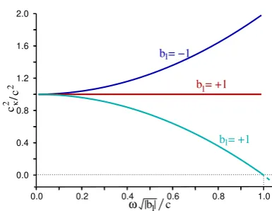
−1. The alternative case whereb1is positive is shown on
fig. 3, where the low-wavevector limit is simplyc2. In the
high-wavevector limitc2
Ωtends tob2/b1, meaning that for
σ <0 (the usual case) only low-k waves propagate. For the spatially propagated ERE wave, the refer-ence wave speed has a much simpler behaviour; although this simplicity is counteracted by the corresponding wave equations (e.g. eqns. (4.19) or (4.22)) being less straight-forward. The reference wave vectorκ2gives a wave speed
c2κ=ω2/κ2=c2 1−b1ω2/c2. (4.24)
In the low-frequency limit this is simplyc2, but that the other limit is more complicated. For a high enough fre-quency (or large enough b1, so that b1ω2 =c2) the
ref-erence wave speed vanishes. For higher frequencies, the wave becomes evanescent, sinceκ2is negative and hence
κis imaginary. These are shown on fig. 4.
Between the two choices of propagation direction (i.e. either of time or of space) we can see that the partitioning
c
2
cΩ
2
b1
k
b
1> 0
/
Stop band forσ = −10 Stop band forσ = −1
0 2 4 6 8 10
0.0 1.0 2.0 3.0 4.0
σ = +10
σ = +1
σ = −10 σ = −1
[image:8.595.342.539.51.190.2]0
FIG. 3: The temporally propagated ERE reference wave speed c2Ω, in theb1 >0 case, for selectedσ. Ifc2Ω <0, the
waves do not propagate, but instead decay (dashed lines).
c
2
cκ
2 /
b = +11 b = +1
1
b = −11
0.0 0.4 0.8 1.2 1.6 2.0
0.0 0.2 0.4 0.6 0.8 1.0
c
ω b1
FIG. 4: Thespatially propagated ERE reference wave speed c2κas a function of frequency for selected b1. Ifc2κ <0, the waves are evanescent (dashed line), and do not propagate; this occurs forω2b1/c2>1.
of terms leading to the reference frequency or wavevec-tor are not the same. Theb2 term only appears in the
reference behaviour for the choice of temporal propaga-tion, but theb1term appears in both. Lastly, despite the
differing sign of theb1 term (or rather, because of it), to
first order inkorω, either reference behaviour gives the same dispersion.
[image:8.595.340.533.270.419.2]V. THE STOKES’ AND THE VAN WIJNGAARDEN’S EQUATIONS
The propagation of an acoustic velocity field is com-monly described by the Stokes’ equation [3], which can even be be extended to describe propagation of acoustic waves in an isothermal, viscous, bubbly liquid [34]. This extension was first done for one dimension by van Wi-jngaarden [4], hence the “van WiWi-jngaarden’s equation” (VWE), but has also been generalized to three dimen-sions [35]. However, the 3D VWE differs from the com-mon form of the Stokes’ equation in that it has spatial operators of ∇∇ ·g and not ∇2g. Here, to allow for a
compact description that includes the 3D Stokes’ equa-tion, but remains compatible with the 1D VWE, a hybrid Stokes’/ VWE equation (S/VWE) for the velocity poten-tialg≡g(~r, t) is introduced. It is
∇2g− 1
c2∂ 2
tg+γ∂t∇2g+β2∂t2∇
2g=Q. (5.1)
Here Qis a source term, such as a driving term or some modification to the wave equation. One could even rec-oncile this equation perfectly with the 3D VWE form [35] if the differences from the ∇2 → ∇∇· substitution
were incorporated in Q, and any side effects properly considered. The equilibrium bubble radius scales as β, despite it having dimensions of time. With β = 0, this becomes the ordinary Stokes’ equation, where the full 3D behaviour of the wave equation is valid. The parameterγ
is proportional to the dynamic viscosity of the (bubbly) mixture. In wavevector-frequency space, withg≡g(~k, ω) andk2=~k·~k=k2
x+k2y+k2z, eqn. (5.1) becomes
k2g− 1 c2ω
2g
−ıγk2ωg−β2k2ω2g=−Q. (5.2)
A. Temporal propagation, spatial decomposition
To decompose the S/VWE into wave components evolving forwards or backwards in space, choose to prop-agating forwards in time. This relies on a suitable refer-ence frequency Ω(k), which results from a careful parti-tioning of the terms in the wave equation (5.2) to give an Ω with only ak dependence. The S/VWE forg(~k, ω) is now written as
c2k2g−ω2
1 +c2β2k2
g=−c2Q+ıc2γωk2g (5.3)
=−Q0, (5.4)
where Ω(k) and the new source termQ0 are defined as
Ω(k)2= c
2k2
1 +c2β2k2, (5.5)
Q0 =
Q/k2−ıγωg
Ω(k)2. (5.6)
Here Ω tends to 1/βin the high-wavevector limit – or is constant at c2k2 in the Stokes’ case where β = 0. Note
c / c
0.0 0.2 0.4 0.6 0.8 1.0
0.0 0.5 1.0 1.5 2.0 2.5 3.0 3.5 4.0
Ω
2
2
[image:9.595.342.537.52.188.2]kc
β
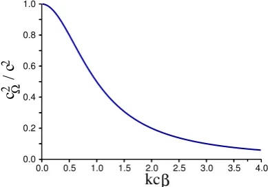
FIG. 5: The S/VWE reference wave speedcΩ = Ω/k as a
function of scaled wavevectorkcβ. In the bubble-free Stokes’ case,β2= 0 and the wave speed is a constant atcΩ/c= 1 for
allk.
that as can be seen on fig. 5 the reference wave speed
c2 Ω= Ω
2/k2 in the same high-wavevector limit decreases
towards zero as 1/kβ, and that the low-wavevector limit is simplyc. Thus all components of the wavevector spec-trum have an ordinary oscillatory (and non-lossy) refer-ence evolution.
Then, as for eqns. (2.5) to (2.7), decompose ginto ve-locity potentialsg+andg− that evolve forward or back-ward in space, withg =g++g−. The two coupled first order wave equations forg±(~k, t) are
ωg±=±Ωg±± 1 2ΩQ
0. (5.7)
Eqn. (5.7) can be transformed so as to apply tog±(~k, t), and becomes
∂tg±=∓ıΩg±∓
ı
2ΩQ
0 (5.8)
=∓ıΩg±∓
ıΩ 2k2Q∓
ıγΩ
2 ∂t(g++g−). (5.9) Here the directedg± evolves as specified by Ω, but that that reference evolution is modified and coupled byQand the dynamic viscosity γ. If the source terms are small, i.e.
Ω
k2Q
, |γΩ∂t(g++g−)| 2|Ωg±|, (5.10)
then the wave evolves slowly as it propagates, so a uni-directional approximation can be made, settingg− = 0. The forward wavesg+(~k, t) then follow
∂tg+=−ıΩg+−
ıΩ 2k2Q−
ıγΩ
B. Spatial propagation, temporal decomposition
To decompose the S/VWE into wave components evolving forwards or backwards in time, choose to prop-agate forwards in space. This uses a suitable reference reference wavevectorκ(ω), resulting from a careful par-titioning of the terms in the wave equation (5.2) to give anκwith only a ω dependence. The S/VWE eqn. (5.2) forg(~k, ω) is now written
c2
1−ıγω−β2ω2
k2g−ω2g=−c2Q (5.12)
k2g−κ0(ω)2g=−
c2κ 0(ω)2
ω2 Q, (5.13)
and if the propagation axis lies alongx, this becomes
k2xg−κ0(ω)2g=−
c2κ 0(ω)2
ω2 Q−k 2
Tg. (5.14) In both eqns. (5.13) and (5.14) the reference wavevector
κ0(ω) is defined as
κ0(ω)2=
ω2/c2
1−ıγω−β2ω2. (5.15)
The S/VWE eqn. (5.14) contains an imaginary part in its reference wavevectorκ0, which is not always desirable.
This can be circumvented by splitting κ20 into real and
imaginary parts using κ20=κ2R+ıκI, and moving κI to the RHS4:
κ0(ω)2=
1−β2ω2
ω2/c2
(1−β2ω2)2−γ2ω2 +
ıωγ ω2/c2
(1−β2ω2)2−γ2ω2
(5.16) =κR(ω)2+ıκI(ω), (5.17)
The S/VWE can then be re-expressed as
k2g−κ2Rg=−c
2κ2
R
ω2
1 + ıωγ 1−β2ω2
Q+ıκI(ω)g,
(5.18) although it will also be convenient to merge theκI term into theQterm as follows
k2g−κ2Rg=−c
2κ2
R
ω2 QR, (5.19)
QR=Q
1 + ıωγ 1−β2ω2
− ıω
3γ/c2
1−β2ω2g. (5.20)
If the propagation axis is alongx, the RHS of the wave equation (still forg(~k, ω)) can be written in either of two forms, namely
k2xg−κ2R(ω)g=−c
2κ
R(ω)2
ω2 QR−k 2
Tg (5.21)
=−c
2κR(ω)2
ω2 Q
1 + ıωγ 1−β2ω2
+ıκIg−k2Tg.
(5.22)
4 Note the imaginaryκ
I part isnot squared
Let us proceed without deciding yet whetherκ0andQ
(as in eqn. (5.14)) orκR and QR (as in eqn. (5.21)) is the best choice. To achieve this, a subscript-free κand
Q0 are used to stand in for whichever pair of{κ0, Q} or
{κR, QR}is convenient, noting that the RHS is given by either of
c2κ0(ω)2
ω2 Q
0= c2κ0(ω)2
ω2 Q+k 2
Tg, (5.23)
or c
2κ
R(ω)2
ω2 Q
0= c2κR(ω)2
ω2 Q−ıκI(ω)g+k 2
Tg (5.24)
= c
2κR(ω)2
ω2 QR+k 2
Tg. (5.25)
If a physical justification could be imagined, this spatial decomposition would allow the parametersc, β, γto have a dependence onω, although the appropriately matching time dependence would need to be present in eqn. (5.1). Now following the same steps as for eqns. (2.13) to (2.15), decomposeg into velocity potentials g+ and g− that evolve forward or backward in time, withg=g++
g−. The coupled wave equations forg±(~k, ω) are
kxg± =±κg±∓ 1 2
c2κ
ω2Q
0 (5.26)
Eqn. (5.26) can be transformed so as to apply to
g±(x, ky, kz, ω), and becomes
∂xg±=±ıκg±∓
ı
2
c2κ ω2 Q
0. (5.27)
The two possible choices of κ are now addressed sepa-rately.
1. The bareκ0 form
On the basis ofκ2
0, the reference wave speed in the
low-frequency limit is simply c, but the other limit is more complicated. For γ = 0, reference wave speed vanishes atω2= 1/β2, and above this the wave becomes
evanes-cent, since κ2
0 is negative and κ0 imaginary. Choosing
κ=κ0 and Q0 = Q+k2Tg, means that eqn. (5.27) for
g±(x, ky, kz, ω) becomes
∂xg±=±ıκ0g±∓
ıc2κ 0
2ω2 Q (5.28)
=±ıκ0g±∓
ıc2κ 0
2ω2 Q∓
k2
T 2κ0
g++g−. (5.29)
Again, the directedg±evolve as specified byκ0, but that
reference evolution is modified and coupled byQandk2
T. If the source terms are small, i.e.
c2κ 0
2ω2Q
,
k2
T 2κ0
g++g−
2κ0g±
, (5.30)
a unidirectional approximation [6] can be made, with
g− = 0; noting also that the k2
paraxial propagation. The forward wavesg+(x, ky, kz, ω) then follow
∂xg+= +ıκ0g+−
ıc2κ0
2ω2 Q−
k2T
2κ0
g+. (5.31)
2. The dressedκR form
On the basis ofκ2
R, the reference wave speed in the low-frequency limit is simply c, but the other limit is more complicated. For zero dynamic viscosity (i.e. γ = 0), it matches the bare behaviour, although for finite γ the zero-speed transition is brought down down to a lower frequency. Again, above this vanishing reference wave speed the wave becomes evanescent, since κ2
R is nega-tive and so κR imaginary. With κ = κR and Q0 =
QR+kT2g, eqn. (5.27) can be transformed to apply to
g±(x, ky, kz, ω), becoming
∂xg±=±ıκRg±∓
ıc2κ
R 2ω2
1 + ıωγ 1−β2ω2
Q∓ κI
2κR
g++g−
∓ k
2
T 2κR
g++g− (5.32)
=±ıκRg±∓
ıc2κ
R 2ω2
1 + ıωγ 1−β2ω2
Q
∓ γω κR/2
1−β2ω2 g
++g−
∓ k
2
T 2κR
g++g−
(5.33)
Here the directed g± evolve as specified by κ, but that that reference evolution is modified and coupled byQ,γ, andk2T. If the source terms are small, i.e.
c2
ω2
1 + ıωγ 1−β2ω2
Q
2g±
, (5.34)
γω (g++g−) 1−β2ω2
2g±
(5.35)
and
k2
T
κ2
R
g++g−
2g±
, (5.36)
then the wave evolves slowly as it propagates. Note that the constraint on the Q term in eqn. (5.34) will fail at low frequencies; also that for non-zeroγ, both theQand the dynamic viscosity (eqn. (5.35)) conditions will fail near ω2β2'1. Eqn. (5.36) is equivalent to demanding paraxial propagation. If these conditions, and hence the unidirectional approximation hold, it is reasonable to set
g−= 0. The forward wavesg+(x, k
y, kz, ω) then follow
∂xg+= +ıκRg+−
ıc2κ
R 2ω2
1 + ıωγ 1−β2ω2
Q
− γω κR/2
1−β2ω2g +− k
2
T 2κR
g+. (5.37)
Both here in eqn. (5.37) and in the bidirectional eqn. (5.33) there is a non-zeroγ-dependent source term.
0.0 0.2 0.4 0.6 0.8 1.0 −0.4
0.0 0.4 0.8 1.2
2 κ
c / c
2
2 κ
c R
βω
(evanescent) non−propagating waves
propagating waves Im(c )
κ20
γ = 0.10 γ = 0.01
[image:11.595.340.537.52.175.2]γ = 0.00
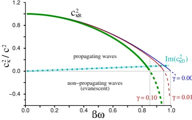
FIG. 6: A comparison of the VWE reference wave speed cκR=ω/κR as a function of frequency for different dynamic viscositiesγ using the continuous lines; note thatcκR=cκ0
ifγ= 0. Dashed lines indicate non propagating (evanescent) regimes. The imaginary part of the wave speed squaredc2
κ0is
indicated by the dash-double-dotted line, for the case where γ = 0.1. The VWE wave speed for γ = 0 andβ = βs is identical to a Stokes’ wave speedcκR ifγ is set equal toβs.
C. Discussion
For this combined S/VWE model, just as for the ERE in section IV, the wave equation is such that each choice of propagation direction results in reference evolutions that differ both conceptually and in practice. This is evident from the reference wave speeds, which are
cΩ(k)2= Ω(k)2/k2=c2/ 1 +c2β2k2
, (5.38)
cκ0(ω)2=ω2/κ0(ω)2=c2 1−ıγω−β2ω2
, (5.39)
cκR(ω)2=ω2/κR(ω)2=c2
1−β2ω22 −γ2ω2
1−β2ω2 . (5.40)
If γ = 0, all describe the same propagation and are in agreement, despite the difference between the high wavevector limit wherecΩ(k→ ∞)→0 and the
transi-tion from propagatransi-tion to evanescence incκ(ω) atβ2ω2= 1. The behaviour of the frequency-dependent forms cκ are shown in fig. 6.
Buckingham [5] takes issue with the physical proper-ties of analytic solutions of the VWE equation, notably its pressure Green’s function; this has non-physical high frequency response when β 6= 0. Since the β2 term in
the VWE has a counterpart in the ERE’s eqn. (4.1)) (i.e. theb1 term), the same remarks could also apply to
that model. However, if the (physically correct) tempo-ral propagation is chosen, and either eqns. (5.9), or eqn. (5.11) areintegrated forward in time – the solution has no choice but to be causal, as long as the loss term∝γ∂t is handled appropriately (or more simply, just neglected). The only spectral information available at a given timet
(e.g. one proportional to a delta function in time), does indeed force ontog(x, t) temporal frequency components above the maximum reference frequency Ωmax= 1/β,but the natural behaviour of the wave equation itself will not. It is then the spatial profile of the impulse that reveals how wave disturbances will evolve forward or backward in space, at finite & bounded speeds cΩ(k) ≤ c. The
step discontinuity reported by Buckingham [5] is not a problem with the wave equation, but an image of the impulsive source term driving the velocity potential.
Another issue relates to the case of non-zeroγ, where that loss has been incorporated in the reference be-haviour. In the discussion in subsection III.D of Bucking-ham [5], the frequency dependent phase speed diverged as cphase '2cβ2ω3/γ for large ω; here this feature can be recovered from the complexκ2
0(ω), since it is spatial
propagation which allows us access to frequency space properties. However, if loss is excluded from κ0 (and
hencecκ0), or is zero, or if the dressedκR(cκR) is used, then no divergence is seen. Instead the phase speed is pure imaginary, corresponding to evanescent (and not propagating) waves. Perhaps most importantly, the wave speedcΩ(k) relevant to temporal propagation exhibits no
such anomaly.
Indeed, given the difficulty of interpreting complvalued wave speeds, it can be helpful to explicitly ex-clude loss-like terms when evaluating phase and group velocities[30]; i.e. only ever calculate real valued wave ve-locities. Directional decompositions are then ideal, since they extract easily understood reference behaviors from complicated wave equations.
VI. CONCLUSION
Temporal and spatial propagation schemes for some typical acoustic wave equations have been compared and contrasted. The comparison enables a better judgment to be made as to which scheme is more practical in a given circumstance – e.g. if reflections are unimportant, a spatially propagated scheme is advantageous due to its more efficient handling of dispersion. Alternatively, for the ERE, temporal propagation incorporates two param-eters (b1,b2) into its reference Ω(k), but spatial
propaga-tion incorporates only one (b1) into κ(ω). This suggests
that for the ERE that temporal propagation is the nat-ural choice, although if material dispersion were present the judgment might well become less simple.
Factorization methods mean that such comparisons can be made in a very transparent way – structurally sim-ilar temporally and spatially propagated wave equations can be compared term by term; just as the exact cou-pled bidirectional wave equations can be compared with the approximate unidirectional form that results from the single (and physically motivated) “slow evolution” assumption. This enables both quantitative and qual-itative judgments to be made as to the significance of approximations, and/or the effect of any “source” terms that perturb or modify the free propagation. Thus these factorized wave equations have practical advantages for systems that are affected by driving terms, additional material dispersion, or nonlinearity – i.e. effects that make a numerical simulation the most practical way of finding a solution.
The potential for two competing ways of analyzing a situation can also add clarity to debate on specific prop-erties of particular acoustic wave equation. As an exam-ple, the apparently non-physical response function for the VWE equation [5] is revealed as an image of the driving impulse, and not of the evolving wave profile. That pro-file is primarily controlled bycΩ(k), and notcκ(ω), since
to be physically correct the waves must be propagated in time.
In summary, directional decompositions have been used to highlight the distinction between the physically accurate choice of temporal propagation and the often more convenient spatial propagation of waves. Some typ-ical wave equations, containing terms for loss and with high-order derivatives have been analyzed, and the han-dling and consequences of these discussed.
Acknowledgments
This work was predominantly done at Imperial Col-lege London, with support from the EPSRC (grant EP/E031463/1) and the Leverhulme Trust (a 2009 Em-bedding of Emerging Disciplines award).
[1] G. Arfken, Mathematical Methods for Physicists (Aca-demic Press Inc., San Diego, 1985), 3rd ed., ISBN 0-12-059820-5.
[2] V. Porubov,
Amplification of Nonlinear Strain Waves in Solids (World Scientific, Singapore, 2003).
[3] G. G. Stokes,
Trans. Cambridge Philos. Soc.8, 287 (1845), http://www.archive.org/
stream/transactionsofca08camb%23page/286/mode/2up. [4] L. van Wijngaarden,
Annu. Rev. Fluid Mech.4, 369 (1972), doi:10.1146/annurev.fl.04.010172.002101. [5] M. J. Buckingham,
J. Acoust. Soc. Am.124, 1909 (2008), doi:10.1121/1.2973231.
[6] P. Kinsler,
Phys. Rev. A81, 013819 (2010), arXiv:0810.5689,
doi:10.1103/PhysRevA.81.013819. [7] P. Kinsler,
arXiv:0909.3407,
doi:10.1103/PhysRevA.81.023808. [8] P. Kinsler (2014),
“What I talk about when I talk about propagation”, arXiv:1408.0128.
[9] V. Grulier, S. Paillasseur, J.-H. Thomas, J.-C. Pascal, and J.-C. L. Roux,
J. Acoust. Soc. Am.126, 2367 (2009), doi:10.1121/1.3216916.
[10] J. M. Mari, T. Blu, O. B. Matar, M. Unser, and C. Cachard,
J. Acoust. Soc. Am.125, 2413 (2009), doi:10.1121/1.3087427.
[11] J. A. Jensen,
J. Acoust. Soc. Am.89, 182 (1991), doi:10.1121/1.400497.
[12] P. M. Morse and K. U. Ingard, Theoretical Acoustics
(McGraw-Hill, New York, 1968).
[13] A. Ferrando, M. Zacares, P. F. de Cordoba, D. Binosi, and A. Montero,
Phys. Rev. E71, 016601 (2005), doi:10.1103/PhysRevE.71.016601. [14] L. Infeld and T. E. Hull,
Rev. Mod. Phys. 23, 21 (1951), doi:10.1103/RevModPhys.23.21. [15] D. V. J. Billger and P. D. Folkow,
Wave Motion37, 313 (2003), doi:10.1016/S0165-2125(02)00094-X. [16] S. Z. Peng and J. Pan,
J. Acoust. Soc. Am.115, 467 (2004), doi:10.1121/1.1639905.
[17] B. L. G. Jonsson and M. Norgren, Wave Motion47, 318 (2010), doi:10.1016/j.wavemoti.2009.11.005.
[18] G. Pinton, F. Coulouvrat, J.-L. Gennisson, M. Tanter, J. Acoust. Soc. Am.127, 683 (2010),
doi:10.1121/1.3277190. [19] S. J. Carter,
Phys. Rev. A51, 3274 (1995), doi:10.1103/PhysRevA.51.3274. [20] P. Kinsler,
J. Opt.20, (to appear) (2018), doi:10.1088/2040-8986/aaa0fc arXiv:1501.05569.
[21] P. Kinsler,
J. Opt. Soc. Am. B 24, 2363 (2007), doi:10.1364/JOSAB.24.002363;
the arXiv:0707.0986 version has an additional appendix..
[22] E. A. Zabolotskaya and R. V. Khokhlov, Sov. Phys. Acoust.15, 35 (1969). [23] V. P. Kuznetsov,
Sov. Phys. Acoust.16, 467 (1971). [24] B. Fornberg,
A Practical Guide to Pseudospectral Methods
(Cambridge University Press, Cambridge, 1996), ISBN 0-521-49582-2.
[25] J. C. A. Tyrrell, P. Kinsler, G. H. C. New, J. Mod. Opt.52, 973 (2005),
doi:10.1080/09500340512331334086.
[26] P. Kinsler, S. B. P. Radnor, J. C. A. Tyrrell, G. H. C. New,
Phys. Rev. E75, 066603 (2007), arXiv:0704.1212v1,
doi:10.1103/PhysRevE.75.066603. [27] P. R. Stepanishen and K. C. Benjamin,
J. Acoust. Soc. Am.71, 803 (1982), also erratum: doi:10.1121/1.388692, doi:10.1121/1.387606.
[28] E. G. Williams and J. D. Maynard, J. Acoust. Soc. Am.72, 2020 (1982), doi:10.1121/1.388633.
[29] P. Kinsler,
Eur. J. Phys.32, 1687 (2011), doi:10.1088/0143-0807/32/6/022;
the arXiv:1106.1792 version has additional appendices. [30] P. Kinsler,
Phys. Rev. A79, 023839 (2009), arXiv:0901.2466,
doi:10.1103/PhysRevA.79.023839.
[31] P. Kolat, B. T. Maruszewski, K. V. Tretiakov, and K. W. Wojciechowski,
Phys. Stat. Sol. B247, 148 (2010), doi:10.1002/pssb.201083983. [32] R. Lakes,
Science235, 1038 (1987),
doi:10.1126/science.235.4792.1038. [33] M. A. Ajaib (2013),
arXiv:1302.5601,
http://arxiv.org/abs/1302.5601. [34] P. M. Jordan and C. Feuillade,
Phys. Lett. A350, 56 (2006), doi:10.1016/j.physleta.2005.10.004. [35] A. C. Eringen,