Projection Results for the
k-Partition Problem
Jamie Fairbrother∗ Adam N. Letchford†
To Appear in Discrete Optimization
Abstract
Thek-partition problem is anN P-hard combinatorial optimisation problem with many applications. Chopra and Rao introduced two inte-ger programming formulations of this problem, one having both node and edge variables, and the other having only edge variables. We show that, if we take the polytopes associated with the ‘edge-only’ formulation, and project them into a suitable subspace, we obtain the polytopes associated with the ‘node-and-edge’ formulation. This result enables us to derive new valid inequalities and separation algorithms, and also to shed new light on certain SDP relaxations. Computational results are also presented.
Keywords: graph partitioning; polyhedral combinatorics; branch-and-cut; semidefinite programming.
1
Introduction
The k-partition problem (k-PP) is a strongly N P-hard combinatorial opti-misation problem, first defined in [5]. We are given an undirected graphG, with vertex setV and edge set E, a rational weightwefor each edge e∈E,
and an integerkwith 2≤k≤ |V|. The task is to partitionV intokor fewer subsets (called “clusters”), such that the sum of the weights of the edges that have both end-vertices in the same cluster is minimised. Thek-PP has applications in statistical clustering, numerical linear algebra, telecommu-nications, VLSI layout, sports team scheduling and statistical physics (see, e.g., [14, 18, 31]).
Note that thek-PP is equivalent to themax-k-cutproblem, in which one wishes to maximise the sum of the weights of the edges that haveexactly one
end-vertex in the same cluster (see [15]). In particular, whenk= 2, we have the well-known max-cut problem, which is known to be strongly N P-hard
∗
STOR-i Centre for Doctoral Training, Lancaster University, Lancaster LA1 4YF, United Kingdom. E-mail: [email protected]
†
(see [16]). Moreover, the problem of checking whetherGisk-colourable can be reduced to thek-PP. Thus, thek-PP is stronglyN P-hard for all fixedk, and this is so even when k= 3 and G is planar (see again [16]). Not only that, but the special case of the k-PP in whichG is a complete graph and k=|V|, called theclique partitioning problem (CPP), is stronglyN P-hard as well [21].
In their seminal paper [7], Chopra and Rao presented two different 0-1 linear programming (0-1 LP) formulations of the k-PP. One of these for-mulations has both node and edge variables, whereas the other has only edge variables. For each formulation, several families of strong valid linear inequalities (a.k.a. cutting planes) have been discovered (e.g., [7, 8, 11, 21]). For some of these families, we also have efficient separation algorithms (e.g., [3, 4, 12, 27]). There is also a parallel literature concerned withsemidefinite programming(SDP) relaxations of thek-PP (e.g., [14, 15, 18, 25, 31, 33, 34]). The main result in this paper is the following. If we take the polytopes associated with the ‘edge-only’ formulations, and project them into a suit-able subspace, we obtain the polytopes associated with the ‘node-and-edge’ formulations. Although this result is fairly easy to derive, it is very use-ful. Specifically, it leads to new valid inequalities and separation algorithms for the ‘node-and-edge’ formulations, and it sheds new light on the SDP relaxations given in [15, 25, 31].
The paper is structured as follows. A literature review is given in Section 2. The projection results are given in Section 3. The new inequalities and separation algorithms, along with our remarks on SDP relaxations, are presented in Section 4. Some computational results are given in Section 5. Finally, some concluding remarks are given in Section 6.
We use the following (standard) notation throughout the paper. The number of nodes and edges inG is denoted by n and m, respectively. For a given positive integerp, we letKp denote the complete graph onp nodes.
Its vertex set is {1, . . . , p}, which we denote by Vp. Its edge set is denoted
by Ep. We also let Ip, ep and Jp denote the identity matrix of order p,
the all-ones vector with p components, and the (square) all-ones matrix of orderp, respectively. Given a real symmetric matrixM, we writeM 0 to indicate thatM is positive semidefinite (psd).
We also use the following (again standard) terminology. Acliqueis a set of pairwise adjacent nodes. A setC⊆E is a cycle if it induces a connected subgraph ofGin which every node has degree 2. The nodes in the subgraph are denoted byV(C). Two disjoint setsR, S ⊂Eform awheel ifRis a cycle and there exists a node h ∈V \V(R) such that S ={v, h} :v ∈V(R) . (The setRis called therim, the edges inS are calledspokes, andhis called the hub.) Two disjoint sets R, S ⊂ E and an edge {h, h0} ∈ E\R form a
2
Literature Review
We now review the relevant literature. We cover the two 0-1 LP formulations in Subsections 2.1 and 2.2, separation algorithms in Subsection 2.3, and SDP relaxations in Subsection 2.4.
2.1 The node-and-edge formulation
Chopra & Rao [7] present the following 0-1 LP formulation of the k-PP, which has nk+m variables. For eachv∈V and forc= 1, . . . , k, letxvc be
a binary variable, indicating whether nodevlies in thecth cluster. Also, for eache∈E, letye be a binary variable, indicating whether the end-nodes of
elie in the same cluster. Then:
min P
e∈Eweye (1)
s.t. Pk
c=1xvc= 1 (v∈V) (2) yuv≥xuc+xvc−1 ({u, v} ∈E, c= 1, . . . , k) (3)
xuc≥xvc+yuv−1 ({u, v} ∈E, c= 1, . . . , k) (4)
xvc≥xuc+yuv−1 ({u, v} ∈E, c= 1, . . . , k) (5)
xvc∈ {0,1} (v∈V, c= 1, . . . , k) (6)
yuv∈ {0,1} ({u, v} ∈E). (7)
We will let Pxy(G, k) denote the associated polytope, i.e., the convex hull
inRnk+m of pairs (x, y) satisfying (2)–(7). We remark that the inequalities
(4) and (5) can be removed when all of the edge weights are non-negative, but this leads to a different polytope, which has not been studied.
Chopra and Rao show that the inequalities (3)–(5), together with non-negativity constraints, define facets of Pxy(G). They also show that the following inequalities define facets fork≥3:
• Clique inequalities, which take the form:
X
u,v∈C
yuv≥
t+ 1 2
r+
t 2
(k−r), (8)
for all C ⊆ V inducing a clique in G with t = b|C|/kc ≥ 1 and r=|C|modk6= 0.
• Cycle inequalities, which take the form:
yf ≥
X
e∈C\{f}
ye− |C|+ 2, (9)
• Odd wheel inequalities, which take the form:
X
e∈R
ye≥
X
e∈S
ye− b|R|/2c, (10)
for allR, S forming a wheel inG with|R| ≥3 and odd.
• Odd bicycle wheel inequalities, which take the form:
yhh0 +
X
e∈S
ye≥
X
e∈R
ye−(|R| −1), (11)
for allR, S,{h, h0} forming a bicycle wheel in Gwith|R|odd.
• Odd cycle inequalities:
X
e∈C
ye≥
X
v∈V(C)
xic− b|C|/2c, (12)
for all cyclesC ⊆E with |C|odd, and for c= 1, . . . , k.
2.2 The edge formulation
Chopra & Rao [7] also presented the following 0-1 LP formulation. Add dummy edges (of zero weight) so thatG becomesKn. Have oney variable
for each e∈En, but nox variables. Then:
min P
e∈Eweye (13)
s.t. yuv ≥yuw+yvw−1 ({u, v, w} ⊂Vn) (14)
P
u,v∈Cyuv≥1 (C⊂Vn: |C|=k+ 1) (15)
ye∈ {0,1} (e∈En). (16)
Note that the constraints (14) are equivalent to the inequalities (9) when G=Kn, and the constraints (15) are a special case of the inequalities (8).
We will letPy(Kn, k) denote the associated polytope.
By definition, any valid inequality for Pxy(Kn, k) that involves only y
variables is valid also forPy(Kn, k). This includes not only the inequalities
(14), (15), but also inequalities (8), (10) and (11). Still more inequalities for Py(Kn, k) are presented in [8, 11].
The polytopePy(Kn, n), called theclique partitioning polytope, has been
studied in depth [1, 11, 12, 20, 21, 22, 28, 29, 30, 32]. Among the many families of strong valid inequalities known for it are, e.g., the 2-partition
and2-chorded odd cycle inequalities [21] and theweighted (s,T)inequalities [30]. Note that any valid inequality forPy(Kn, n) is valid also forPy(Kn, k)
and Pxy(Kn, k) for all k≤n.
do not know of such a formulation for 2 < k < n. (When k = 2, one can use the standard formulation of the max-cut problem [2]. Whenk=n, the cycle inequalities are enough to get a formulation [6].) We return to this issue in Subsection 3.1.
2.3 Separation algorithms
For a given family of inequalities, a separation algorithm is a routine that takes a solution of an LP relaxation as input, and searches for violated in-equalities in that family [19]. Chopra and Rao [7] point out that separation can be done in polynomial time for the cycle inequalities (9) and odd cy-cle inequalities (12) using the approach in [2]. Separation is N P-hard for the clique inequalities (8), by a trivial reduction from the maximum clique problem [13]. Heuristics for clique separation are presented in [13, 24]. Deza
et al. [12] show that separation for the odd wheel inequalities (10) can be done in polynomial time, and point out that separation for the odd bicycle wheel inequalities (11) can also be done in polynomial time, by adapting the approach in [17].
The complexity of separation for the other known families of inequalities is unknown. Separation heuristics for 2-partition and weighted (s, T) in-equalities are given in [20] and [30], respectively. It is shown in [3, 4, 27, 29] that one can separate in polynomial time over various families of valid in-equalities that include all 2-chorded odd cycle inequalities.
2.4 SDP relaxations
Finally, we briefly review SDP relaxations of thek-PP. Freize & Jerrum [15] use the relaxation:
min k−1k P
e∈Ewe
Ye + k−11
s.t. diag(Y) =en
Ye≥ k−1−1 (e∈En)
Y 0.
The idea here is thatY represents a feasible solution ifYuv takes the value
1 when nodesu and v are in the same cluster, and −1/(k−1) otherwise. Observe that Y is related to the vector y in the edge formulation via the identities ye = k−1k Ye+k1 and Ye = k−1k ye− k−11 for all e∈En. Using
these mappings, valid inequalities for Py(Kn, k) can be used to strengthen
following equivalent, yet more natural SDP:
min P
e∈EweY˜e
s.t. diag( ˜Y) =en
˜
Yuv ≥0 ({u, v} ∈En)
kY˜ −Jn0.
Here, ˜Ye plays the same role asye in the edge formulation.
De Klerk et al. [25] consider an alternative approach. Let z ∈ {0,1}nk
be a vector such that, forv= 1, . . . , nandc= 1, . . . , k, nodenlies in cluster cif and only if the component of z in position n(c−1) +v takes the value 1. From a consideration of the matrix
1 z
1 z
T
=
1 zt z zzT
,
they derive an SDP relaxation in which the matrix variable is of ordernk+1. It is shown in [25] that this relaxation gives the same lower bound as the relaxations mentioned above, but provides extra information that can be exploited in an approximation algorithm.
Finally, we mention two recent papers. Van Dam & Sotirov [10] examine an SDP relaxation whose solution has a closed form (involving Eigenvalues). De Sousaet al. [34] show empirically that odd wheel and odd bicycle wheel inequalities can be useful for strengthening SDP relaxations.
3
The Projection Results
In this section, we present our projection results. We proceed in two steps, which are covered in the following two subsections.
3.1 From Pxy(G, k) and Py(K
n, k) to Py(G, k)
We start with the following definition.
Definition 1 Let G = (V, E) be an undirected graph with n nodes and m
edges. The projection ofPxy(G, k) intoy-space, which is also the projection of Py(K
n, k) into Rm, will be denoted by Py(G, k).
Finding valid and even facet-defining inequalities for Py(G, k) is rather easy, as shown by the following two lemmas.
Proof. These inequalities are valid forPxy(G, k) and have zero coefficients
for all xvariables.
Lemma 2 Any valid inequality for Py(Kn, k) is valid also for Py(G, k),
provided that the variables with non-zero coefficients correspond to edges in
E.
Proof. This follows directly from the fact that Py(G, k) is the projection
ofPy(Kn, k) intoRm.
So, for example, the 2-partition, 2-chorded odd cycle and weighted (s, T) inequalities are valid for Py(G, k) whenever G contains the corresponding graph as a subgraph.
The main reason that we are interested in Py(G, k) is that, as we will see in the next subsection, valid inequalities for Py(G0, k), where G0 is a suitable graph, can be used to derive new valid inequalities for Pxy(G). There is however another motivation for studying Py(G, k): it is possible to compute lower bounds for the k-PP with a cutting-plane algorithm that has only m variables, in which the cutting planes are valid inequalities for Py(G, k).
Now, recall from the end of Subsection 2.2 that, for 2< k < n, Chopra and Rao were unable to find a formulation of the k-PP that uses only m variables. In fact, a simple formulation is:
min P
e∈Eweye
s.t. yf ≥
P
e∈C\{f}ye− |C|+ 2 (C ∈ C, f ∈C)
P
e∈Fye≥1 (F ∈ F)
ye∈ {0,1} (e∈E),
where C contains all chordless cycles C ⊂ E, and F contains all minimal sets F ⊂ E that induce a subgraph of G that is not k-colourable. Unfor-tunately, this formulation seems to be of little practical use, since testing k-colourability isN P-hard.
To close this subsection, we remark that, when k = 2, the polytope Py(G, k) reduces to the cut polytope of G (or, more precisely, a reflection of the cut polytope, obtained by complementing all variables). In [2], it is shown how to obtain new facets of the cut polytope from old ones, by applying graph operations such as “edge subdivision” and “node splitting”. We suspect that one could obtain new facets of Py(G, k) in a similar way, but we do not explore this here, for brevity.
3.2 From Py(G, k) (almost) to Pxy(G, k)
Definition 2 Given a graph G = (V, E) and a positive integer k, the “k-augmented graph”, denoted by Gk, is a graph with node setV ∪ {d1, . . . , dk}
and edge set D∪E∪F, where D = {v, dc} : v ∈ V, c = 1, . . . , k and
F =
{dc, dc0}: 1≤c < c0 ≤k . The nodes d1, . . . , dk are called “dummy” nodes. The edges in D and F are called “dummy” edges and “forbidden” edges, respectively.
Lemma 3 Suppose thaty ∈ {0,1}|D|+|E|+|F|is an extreme point ofPy(Gk, k)
such that ye = 0 for all forbidden edges e∈F. Then, in the corresponding
k-PP solution, there are exactlykclusters, and exactly one dummy node lies in each cluster.
Proof. From the definition ofF, we haveye= 0 for every edge connecting
two dummy nodes. This means that no two dummy nodes can lie in the same cluster, which implies in turn that each dummy node lies in a separate cluster. The result then follows from the fact that there arekdummy nodes, and the fact that a feasiblek-PP solution has no more thank clusters.
The main result in this section is then the following.
Theorem 1 For a given G and k, let Gk be the corresponding augmented
graph. Suppose we takePy(Gk, k) and perform the following operations: 1. Take the face of Py(Gk, k) induced by the hyperplanes ye = 0 for all
e∈F.
2. Project the face into RD+E.
3. For each dummy edge e={v, dc}, change the name of the variable ye
toxvc.
The resulting polytope is Pxy(G, k).
Proof. From Lemma 3, every extreme point of Py(Gk, k) lying on the stated face corresponds to ak-partition in which exactly one dummy node lies in each cluster. For c= 1, . . . , k, let us call the cluster containing node dc “cluster c”. Then, for any given dummy edge e={v, dc} ∈D, ye= 1 if
and only if node v lies in cluster c, i.e., if and only if xvc = 1 in the node
and edge formulation. Moreover,|D|=nk, and therefore the projection lies inRnk+m, the same space in which Pxy(G, k) lies.
Theorem 1 has the following useful corollary:
Corollary 1 If the inequality αTy ≤ β is valid for Py(Gk, k), then the “projected” inequality
X
e={v,dc}∈D
αexvc +
X
e∈E
αeye ≤ β
Corollary 1 sheds light on the valid inequalities for Pxy(G, k) given in Chopra & Rao [7]. In particular:
• The inequalities (14) are valid for Py(Gk, k), provided that {u, v, w}
induces a triangle in Gk. If we assume that {u, v} ∈ E and identify nodew with the dummy nodedc, we obtain the inequalities (3).
• If instead we assume that {u, w} ∈ E and identify node v with the dummy nodedc, we obtain (up to a relabelling of the remaining nodes)
the inequalities (4) and (5).
• The odd wheel inequalities (10) are valid forPy(Gk, k), provided that Gk contains the odd wheel as a subgraph. If we assume that R ⊆ E and identify the hub h with the dummy node dc, we obtain the odd
cycle inequalities (12).
Further implications of Theorem 1 and Corollary 1 are given in the next section.
We remark that a necessary condition for a “projected” inequality to define a facet of Pxy(G, k) is that the original inequality defines a facet of Py(Gk, k). We do not know whether this condition is also sufficient.
4
Implications
In this section, we show how the results of the previous subsection lead to new valid inequalities and separation algorithms for the node-and-edge formulation. We also make some remarks about SDP relaxations.
4.1 New valid inequalities
One way to derive new valid inequalities forPxy(G, k) is to use Lemma 1 to project from Pxy(Gk, k) to Py(Gk, k), and then use Corollary 1 to project from Py(Gk, k) to Pxy(G, k). Here is an example. Let T ⊆V be a clique in G, let S be any subset of {1, . . . , k}, and let S0 = {dc : c ∈ T} be the
corresponding set of dummy nodes inGk. By construction,C =T∪S0forms a clique inGk. Then, provided thatt=b|C|/kc ≥1 andr=|C|modk6= 0, the clique inequality (8) defines a facet ofPxy(Gk, k). By Lemma 1, it also defines a facet of Py(Gk, k). Corollary 1 then yields the following valid inequality for Pxy(G, k):
X
v∈T
X
c∈S
xvc+
X
u,v∈T
yuv≥
t+ 1 2
r+
t 2
(k−r). (17)
We call inequalities of this typeprojected clique inequalities.
Lemma 4 IfS ={1, . . . , k}, then the projected inequality (17) is equivalent to the clique inequality onT.
Proof. Consider what would happen if we changed S from{1, . . . , k} to∅. The effect on the left-hand side of (17) is that the term involvingxvariables would disappear. Due to the equations (2), the net decrease in the left-hand side would be |S|. As for the right-hand side of (17), note that the stated change in S causes us to remove the elements of S0 from C, which in turn causes t to decrease by 1. As a result, the net decrease in the right-hand side istr+ (t−1)(k−r) = (tk+r)−k=|C| −k=|S|.
For 1≤ |S|< k, the projected clique inequalities are new. Moreover, we have the following result.
Theorem 2 Projected clique inequalities define facets of Pxy(G, k).
Proof. See A.
In a similar way, one can derive projected versions of the cycle, odd wheel and odd bicycle wheel inequalities. For the sake of brevity, we do not explore this in detail here. We note however that:
• The only projected cycle inequalities that define facets are the cycle inequalities themselves. (This is because a cycle that passes through a dummy node inGk can never be chordless.)
• The odd cycle inequalities (12) are an example of facet-defining pro-jected odd wheel inequalities. (This follows from the remark at the end of Section 3.)
Another way to derive new valid inequalities for Pxy(G, k) is to take a family of valid inequalities for the clique partitioning polytopePy(Kn+k, n),
note that they are valid also forPy(Kn+k, k), use Lemma 2 to find out when
they are valid also forPy(Gk, k), and finally use Corollary 1 to project them fromPy(Gk, k) toPxy(G, k). Here is an example. Oostenet al.[30] showed that, for any setT ⊂V with|T| ≥3, any nodes∈V \T, and any integer α between 1 and |T| −2, the following weighted (s, T) inequality defines a facet ofPy(Kn, n):
X
u,v∈T
yuv≥α
X
v∈T
ysv−
α+ 1 2
.
It is valid, though not necessarily facet-defining, also for Py(Kn+k, k). By
Now, if we identify s with a dummy node, say dc, Corollary 1 yields the
following valid inequality forPxy(G, k):
X
u,v∈T
yuv≥α
X
v∈T
xvc−
α+ 1 2
. (18)
We call inequalities of this typeweighted clique inequalities.
The weighted clique inequalities are valid for allk≥2, all cliquesT ⊆V with |T| ≥ 3, all cluster indices c ∈ {1, . . . , k}, and all α between 1 and
|T|−2. It turns out that they define facets ofPxy(G, k) whenαis sufficiently
large.
Theorem 3 Weighted clique inequalities define facets of Pxy(G, k) if and only ifk≥3 and |T| −k < α≤ |T| −2.
Proof. See B.
We remark that the inequalities (14) can be regarded as ‘degenerate’ weighted (s, T) inequalities with|T|= 2 andα= 1, and the inequalities (3) can be regarded as ‘degenerate’ weighted clique inequalities with |T| = 2 and α= 1.
4.2 New separation algorithms
In addition to new inequalities for the node-and-edge formulation, we obtain new separation algorithms. The key is the following proposition.
Proposition 1 Let F be a family of valid inequalities for Py(Gk, k), and let F0 be the corresponding family of projected inequalities for Pxy(G, k). Also let (x∗, y∗)∈[0,1]nk+m be a solution to an LP relaxation of the node-and-edge formulation. We construct a pointy˜∈[0,1]nk+m+(k2) by settingy∗ e
to:
• x∗vc if e={v, dc} for some v∈V and c∈ {1, . . . , k},
• y∗e if e∈E,
• 0 if e={dc, dc0} for some c, c0 with1≤c < c0 ≤k.
Theny˜violates an inequality inF if and only if(x∗, y∗)violates an inequality in F0.
Proof. This follows from Theorem 1 and the definition of “projected”
Example: Suppose that k = 3 and G = K3. Setting x∗12, x∗13, x∗22, x∗23, x∗32, x∗33 to 1/2 and all other variables to zero, we obtain a pair (x∗, y∗) that satisfies all of the inequalities mentioned in Subsection 2.1. Using the mapping in the proposition, we obtain a point ˜y with
˜
y1,d2 = ˜y1,d3 = ˜y2,d2 = ˜y2,d3 = ˜y3,d2 = ˜y3,d3 = 1/2
and all other variables equal to zero. This point violates the following clique inequality by 1:
y1,d1+y2,d1 +y3,d1 +y12+y13+y23≥1.
The corresponding projected clique inequality is
x11+x21+x31+y12+y13+y23≥1.
The point (x∗, y∗) violates it by 1.
We have the following corollary.
Corollary 2 There exist polynomial-time separation algorithms for pro-jected odd wheel and propro-jected odd bicycle wheel inequalities, and for a family of inequalities that includes all projected 2-chorded odd cycle inequalities.
Proof. This follows from Proposition 1 and the known results mentioned in Subsection 2.3. There is however one minor complication in the case of the third family of inequalities mentioned: the separation algorithms given in [3, 4, 27] assume that the underlying graph is complete, but the graph Gk need not be complete. Fortunately, the separation algorithm given in [29] works on general graphs, and the algorithms in [3, 4, 27] can be easily
adapted to the case of general graphs.
In a similar way, the heuristics for clique, 2-partition and weighted (s, T) separation, mentioned in Subsection 2.3, can be used to derive heuristics for the corresponding projected inequalities.
4.3 On SDP relaxations
We now present a modified SDP relaxation for thek-PP. Although we are not yet sure whether it is of any practical value in itself, we will see that it yields a new family of valid inequalities for Pxy(Kn, k), along with an
efficient separation algorithm for them. LetX ∈ {0,1}nk be a matrix in whichX
vc= 1 if and only if nodev lies
in cluster c. (Rendl [31] calls X a partition matrix.) Note that Xvc plays
the same role as xvk in the node-and-edge formulation, and thatXek=en.
Now consider the matrix:
Z =
Ik
X Ik
X
T
=
Ik XT
X XXT
By definition, this matrix is psd. Moreover, the submatrixXXT is nothing but the matrix ˜Y used in Rendl’s SDP relaxation. This leads naturally to the following SDP relaxation:
min P
e∈EweY˜e
s.t. diag( ˜Y) =en
˜
Yuv ≥0 ({u, v} ∈En)
Xek =en
Z =
Ik XT
X Y˜
0.
Note that this relaxation involves a matrix variable of orderk+n. We have the following proposition:
Proposition 2 The new SDP relaxation gives the same lower bound as the Freize–Jerrum SDP relaxation (and therefore also the Rendl and De Klerk
et al. relaxations).
Proof. As mentioned in Subsection 2.4, the Freize–Jerrum, Rendl and De Klerket al. relaxations all give the same bound. Now, let ˜Y∗ be a feasible solution to Rendl’s relaxation. Suppose we set Xvc∗ to 1/k for all v and c. Then our claim is that the pair (X∗,Y˜∗) is a feasible solution to the new relaxation. To see this, note that all linear constraints are satisfied. As for the psd constraint on Z, Schur complement implies that Z 0 if and only if ˜Y −XXT 0. But this latter constraint is satisfied by (X∗,Y˜∗), since kY˜∗−Jn0 and X∗(X∗)T =Jn/kby construction.
Now, let (X∗,Y˜∗) be a feasible solution to the new relaxation. Since the corresponding matrixZ∗ is psd, we have
a b
Ik (X∗)T
X∗ Y˜∗ a b
T
≥ 0 (19)
for all a∈ Rk and b ∈
Rn. Now consider what happens if we set ato ek
for some∈R. Since ekIkekT =kand X∗ek=en, the inequality (19) then
reduces to:
b
k en
en Y˜∗
b
T
≥ 0.
Since this true for alland allb, we have:
k en
en Y˜∗
0.
By Schur complement, this is equivalent to kY˜∗ −Jn 0. Thus, ˜Y∗ is
As mentioned above, it is not clear to us whether the new relaxation could be of practical use in itself. Although it gives the same bound as Rendl’s relaxation, the matrixX∗ gives additional information, which could perhaps be exploited in a randomised rounding heuristic for the k-PP. We leave this as a possible topic for future research. Our main interest in the new relaxation is that it leads to new valid inequalities forPxy(Kn, k), along
with an efficient separation algorithm for them.
Proposition 3 The following “psd” inequalities are valid for Pxy(Kn, k),
for alla∈Rk and b∈
Rn:
k
X
c=1
X
v∈V
acbvxvc+
X
{u,v}∈E
bubvyuv≥ − ||a||22+||b||22
/2.
Proof. This follows from the inequalities (19), the definition ofZ, the fact that X encodes the x variables, the fact that diag( ˜Y) = en, and the fact
that the off-diagonal elements of ˜Y encode they variables.
Proposition 4 The separation problem for the psd inequalities can be solved in polynomial time (to arbitrary precision).
Proof. Let (x∗, y∗) be the point to be separated, with x∗ ∈ [0,1]kn and
y∗ ∈ [0,1](n2). Construct the corresponding matrix Z∗, and compute its
minimum Eigenvalue to the desired precision. If the Eigenvalue is positive, Z∗ is psd, and therefore no psd inequality is violated. Otherwise, let ab be the associated Eigenvector, wherea∈ Rk and b ∈
Rn. The inequality (19)
is violated byZ∗, and therefore the corresponding psd inequality is violated
by (x∗, y∗).
We remark that a similar argument was used in [26] to derive valid inequal-ities for the cut polytope, or, equivalently, for Py(K
n,2), along with an
efficient separation algorithm for them.
We close this section with two further remarks. First, the psd inequalities are valid for Pxy(G, k) even whenG is not complete, as long as the nodes
with non-zerobv values form a clique inG. Second, if one takes the so-called
hypermetric inequalities for Py(Kn, k), presented in [8], and then applies
our projection procedure, the resulting projected hypermetric inequalities forPxy(Kn, k) dominate the psd inequalities. We skip the details, partly for
brevity, and partly because the complexity of separation for the hypermetric inequalities is unknown.
5
Computational Experiments
computer with a 4-core Intel Core i5-4690 CPU clocked at 3.50GHz and running under Linux with kernel version 4.4. We used the software package
igraph[9] to construct graphs and enumerate maximal cliques, andGurobi
version 7 [23] to solve all LPs and 0-1 LPs.
5.1 Test instances
Recall that the “node-and-edge” formulation is most suitable for k-PP in-stances in whichGis sparse. We therefore constructed ten sparse disk graphs as follows. We take the unit torus and place 50 nodes at random. We then include an edge between a given pair of nodes if and only if their Euclidean distance exceeds a constant r. (We chose r = 0.25, which led to graphs with average degree around 9.5.) Each edge in the resulting graph is given a random integer weight between 1 and 10. For each of the ten graphs, we then consideredk∈ {2,3,4}. This makes 30k-PP instances in total.
The motivation for restricting attention to k-PP instances with positive edge weights is that clique inequalities work well for such instances. For instances with a mixture of positive and negative weights, other families of inequalities (such as odd wheel inequalities) are more useful [34].
5.2 Experimental setup
For each instance, we compare three algorithmic settings:
1. Solve the 0-1 LP problem (1)–(7) by plain branch-and-bound.
2. Run a cutting plane algorithm, in which the separation problem for the clique inequalities (8) is solved by brute-force enumeration. At termination, delete all clique inequalities with slack larger than 0.1 and run branch-and-bound.
3. As in option 2, except that, between the termination of the cutting-plane algorithm and the start of branch-and-bound, we run a second cutting-plane algorithm, in which the separation problem for the pro-jected clique inequalities (17) is solved by enumeration.
For the instances considered, the time taken in the cutting-plane phases was negligible compared to the branch-and-bound time. (For larger instances and/or larger values of k, one would probably have to separate over the clique and projected clique inequalities heuristically, rather than exactly.)
5.3 Results
No Cuts Clique Gen. Clq.
k nodes time nodes time nodes time
[image:16.595.143.453.124.203.2]2 5410.10 15.10 17.30 0.19 15.60 0.20 3 38665.90 157.72 3117.70 3.68 4650.90 9.05 4 210040.60 183.78 3973.80 3.20 30665.40 33.60
Table 1: Branch-and-bound results for random k-PP instances.
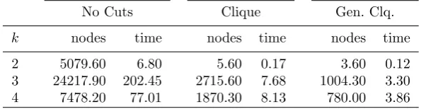
No Cuts Clique Gen. Clq.
k nodes time nodes time nodes time
2 5079.60 6.80 5.60 0.17 3.60 0.12 3 24217.90 202.45 2715.60 7.68 1004.30 3.30 4 7478.20 77.01 1870.30 8.13 780.00 3.86
Table 2: Branch-and-bound results for node-weighted variant.
in both measures. Surprisingly, however, the projected clique inequalities do not lead to any further reduction. In fact they sometimes make things worse.
Examination revealed that the addition of projected clique inequalities that are not ordinary clique inequalities led to no improvement in the lower bound from the LP relaxation. This may be because they involvexvariables, which do not appear in the objective function. To test this hypothesis, we modified the 30k-PP instances by giving eachx variable a random integer cost between 1 and 10. The results obtained are shown in Table 2. We see that, as expected, the projected clique inequalities now lead to a significant improvement.
6
Concluding Remarks
We have shown that known results for the “edge-only” formulation of the k-PP yield, via projection, both known and new results for the “node-and-edge” formulation. In particular, we have obtained several new families of valid inequalities for the latter, along with new separation algorithms. As a by-product, we have obtained a new variant of the SDP relaxations given in [15, 25, 31].
[image:16.595.148.446.248.325.2]perhaps form the basis for a new heuristic. Finally, we believe that more work is needed on valid inequalities and separation algorithms for problems related to thek-PP, such as the clique partitioning problem and other graph partitioning problems.
References
[1] H.-J. Bandelt, M. Oosten, J.H.G.C. Rutten & F.C.R. Spieksma (1999) Lifting theorems and facet characterization for a class of clique parti-tioning inequalities.Oper. Res. Lett., 24, 235–243.
[2] F. Barahona & A.R. Mahjoub (1986) On the cut polytope.Math. Pro-gram., 36, 157–173.
[3] R. Bornd¨orfer & R. Weismantel (2000) Set packing relaxations of inte-ger programs. Math. Program., 88, 425–450.
[4] A. Caprara & M. Fischetti (1996) {0,12}-Chv´atal-Gomory cuts. Math. Program., 74, 221–235.
[5] R. Carlson & G.L. Nemhauser (1966) Clustering to minimize interaction costs. Oper. Res., 14, 52–58.
[6] S. Chopra (1994) The graph partitioning polytope on series-parallel and 4-wheel free graphs. SIAM J. Discr. Math., 7, 16–31.
[7] S. Chopra & M.R. Rao (1993) The partition problem.Math. Program., 59, 87–115.
[8] S. Chopra & M.R. Rao (1995) Facets of thek-partition polytope.Discr. Appl. Math., 61, 27–48.
[9] G. Csardi & T. Nepusz (2006) The igraph software package for complex network research. InterJournal, Complex Systems, 1695, 1–7.
[10] E.R. van Dam & R. Sotirov (2016) New bounds for the max-k-cut and chromatic number of a graph. Lin. Alg. Appl., 488, 216–234.
[11] M. Deza, M. Gr¨otschel & M. Laurent (1991) Complete descriptions of small multicut polytopes. In P. Gritzmann & B. Sturmfels (eds)Applied Geometry and Discrete Mathematics. Providence, RI: AMS.
[12] M. Deza, M. Gr¨otschel & M. Laurent (1992) Clique-web facets for mul-ticut polytopes. Math. Oper. Res., 17, 981–1000.
[14] A. Eisenbl¨atter (2002) The semidefinite relaxation of the k-partition polytope is strong. In W.J. Cook & A.S. Schulz (eds.)Integer Program-ming and Combinatorial Optimization IX, pp. 273–290. Lecture Notes in Computer Science, vol. 2337. Berlin: Springer.
[15] A. Frieze & M. Jerrum (1997) Improved approximation algorithms for max-k-cut and max bisection. Algorithmica, 18, 67–81.
[16] M.R. Garey, D.S. Johnson & L.J. Stockmeyer (1976) Some simplified
N P-complete graph problems. Theoret. Comput. Sci., 1, 237–267.
[17] A.M.H. Gerards (1985) Testing the odd bicycle wheel inequalities for the bipartite subgraph polytope. Math. Oper. Res., 10, 359–360.
[18] B. Ghaddar, M.F. Anjos & F. Liers (2011) A branch-and-cut algorithm based on semidefinite programming for the minimumk-partition prob-lem. Ann. Oper. Res., 188, 155–174.
[19] M. Gr¨otschel, L. Lov´asz & A.J. Schrijver (1988) Geometric Algorithms and Combinatorial Optimization. New York: Wiley.
[20] M. Gr¨otschel & Y. Wakabayashi (1989) A cutting plane algorithm for a clustering problem. Math. Program., 45, 59–96.
[21] M. Gr¨otschel & Y. Wakabayashi (1990) Facets of the clique partitioning polytope. Math. Program., 47, 367–387.
[22] M. Gr¨otschel & Y. Wakabayashi (1990b) Composition of facets of the clique partitioning polytope. In R. Bodendieck & R. Henn (eds.)Topics in Combinatorics and Graph Theory, pp. 271–284. Heidelberg: Physica-Verlag.
[23] Gurobi Optimization, Inc. (2017)Gurobi Optimizer Reference Manual. Available at http://www.gurobi.com
[24] V. Kaibel, M. Peinhardt & M.E. Pfetsch (2011) Orbitopal fixing.Discr. Optim., 8, 595–610.
[25] E. de Klerk, D.V. Pasechnik & J.P. Warners (2004) On approximate graph colouring and max-k-cut algorithms based on the θ-function.J. Comb. Optim., 8, 267–294.
[26] M. Laurent & S. Poljak (1996) Gap inequalities for the cut polytope.
Eur. J. Combinatorics, 17, 233–254.
[28] A.N. Letchford & M.M. Sørensen (2012) Binary positive semidefinite matrices and associated integer polytopes. Math. Program., 131, 253– 271.
[29] R. M¨uller & A.S. Schulz (2002) Transitive packing: a unifying concept in combinatorial optimization. SIAM J. Optim., 13, 335–367.
[30] M. Oosten, J.H.G.C. Rutten & F.C.R. Spieksma (2001) The clique partitioning problem: facets and patching facets. Networks, 38, 209– 226.
[31] F. Rendl (2012) Semidefinite relaxations for partitioning, assignment and ordering problems. 4OR, 10, 321–346.
[32] M.M. Sørensen (2002) A note on clique-web facets for multicut poly-topes. Math. Oper. Res., 27, 740–742.
[33] R. Sotirov (2014) An efficient semidefinite programming relaxation for the graph partition problem.INFORMS J. Comput., 26, 16–30.
[34] V.J.R. de Sousa, M.F. Anjos & S. Le Digabel (2016) Computational study of valid inequalities for the maximumk-cut problem.Ann. Oper. Res., to appear.
A
Proof of Theorem 2
In [7], it is pointed out that a (standard) clique inequality is satisfied at equality by an extreme point ofPxy(G, k) if and only if, in the corresponding k-PP solution, each cluster contains either tort+ 1 nodes fromC. Due to the structure of the augmented graphGk, this implies that aprojectedclique inequality (17) is satisfied at equality by an extreme point of Pxy(G, k) if
and only if the following two conditions hold:
• For allc∈S, thecth cluster contains eithert−1 or tnodes from T.
• For allc∈ {1, . . . , k} \S, thecth cluster contains eithertort+ 1 nodes fromT.
We will call such extreme pointsroots. By abuse of terminology, the corre-spondingk-PP solutions will also be called roots.
Now suppose that all roots satisfy an equation of the formαTx+βTy =γ. We will perform a series of exchange arguments to show that the equation is equivalent to a projected clique inequality (in equation form). Throughout, we assume that 1 ≤ |S| < k, since, if |S| ∈ {0, k}, we obtain a standard clique inequality (see Lemma 4).
(i)|W ∩T|is equal to tifc∈S, and equal to t+ 1 otherwise, (ii) |W0∩T|
is equal tot−1 if c0 ∈ S, and equal to t otherwise. Let u be any node in W. One can check that, if u is any node inW, we can obtain another root by movingu fromW toW0. This yields the equation
αuc+
X
v∈W\{u}:{u,v}∈E
βuv=αuc0+
X
v∈W0:{u,v}∈E
βuv. (20)
Now letu0 be any node inW0\T. If we moveu0 fromW0toW, the equation (20) becomes:
αuc+
X
v∈(W\{u})∪{u0}:{u,v}∈E
βuv=αuc0+
X
v∈W0\{u0}:{u,v}∈E
βuv.
Together with (20), this implies that βuu0 = 0. Applying this argument
repeatedly, we see that βuu0 = 0 for all u ∈ V and all u0 ∈ V \T. This in
turn implies that αuc =αuc0 for all pairs c, c0 and for all u ∈V \T. Thus,
for any u ∈ V \T, the coefficients αuc must take a constant value for all
c ∈ {1, . . . , k}. Since all feasible k-PP solutions satisfy the equations (2), we can assume that this constant is zero for all u∈V \T. In this way, the nodes inV \T can be removed from consideration.
Now let c, c0 be cluster indices with c ∈ S and c0 ∈/ S, and let W and W0 be the corresponding clusters. Consider any root such that |W ∩T|=
|W0∩T|=t. We can obtain another root by taking any node u ∈W ∩T and moving it fromW toW0. This shows that
αuc+
X
v∈(W∩T)\{u}
βuv=αuc0+
X
v∈W0∩T
βuv.
Observe that the right-hand side of this equation contains one moreβ term than the left-hand side. By symmetry, we haveβuv=αuc−αuc0 for allc∈S,
c /∈S and {u, v} ⊂T. This implies in turn thatβuv takes a constant value
for all{u, v} ⊂ T, that αuc takes a constant value for all u∈T and c∈S,
and that αuc0 takes a constant value for all c0 ∈/ S. Since all feasible k-PP
solutions satisfy the equations (2), we can assume that the αuc0 are zero,
which then implies that theαuc are equal to theβuv. Finally, by scaling, we
can assume that theαuc and βuv are equal to one.
B
Proof of Theorem 3
As in the proof of Theorem 2, we call a k-PP solution a root if the corre-sponding extreme point ofPxy(G, k) satisfies the weighted clique inequality (18) at equality.
Consider a feasible k-PP solution such that cluster ccontains exactly t nodes from T. This solution must use at least 2t
both end-nodes inT, and it will use exactly 2t
of those edges if and only if each of the other nodes inT lies in a unique cluster. From this it follows that ak-PP solution is a root if and only if (i) clusterccontains eitherαorα+ 1 nodes fromT, and (ii) each of the other nodes inT lies in a different cluster. This can only happen if there are at least|T| −αclusters, i.e., ifk≥ |T| −α. Moreover, if there wereexactly |T| −αclusters, then all roots would satisfy the equation P
v∈Txvc = α+ 1, and the weighted clique inequality could
not define a facet. This showsα must lie between|T| −k+ 1 and|T| −2 if we want to obtain a facet. This in turn implies that k must be at least 3. So, we have proved necessity.
The proof of sufficiency is similar to that of Theorem 2. For brevity, we only give a sketch. We suppose that all roots satisfy an equation of the form βTx+γTy=δ. An exchange argument, in which nodes inV \T are either included in or excluded from clusterc, enables us to show thatγuv=βvc= 0
whenever v ∈ V \T. Another exchange argument, in which a node u ∈ T is moved between clusters, enables us to show that βuc0 = 0 for all u ∈ T
and for all c0 ∈ {1, . . . , k} \ {c}, and that βuc = −αγuv for all {u, v} ⊂T.
Finally, by scaling, we can assume thatγuv = 1 for all{u, v} ⊂T and that