The Asymptotic Study of Smooth Entropy Support Vector Regression

The Asymptotic Study of Smooth Entropy Support

Vector Regression

Guo-Sheng Hu, Jian-Hua Zhang Shanghai Technical Institute of Electronics and

Information, School of Electronics and Information, Shanghai, China Email: [email protected]

Received December 4, 2011; revised February 22, 2012; accepted February 28, 2012

ABSTRACT

In this paper, a novel formulation, smooth entropy support vector regression (SESVR), is proposed, which is a smooth unconstrained optimization reformulation of the traditional linear programming associated with a ε-insensitive support vector regression. An entropy penalty function is substituted for the plus function to make the objective function con- tinuous, and a new algorithm involving the Newton-Armijo algorithm proposed to solve the SESVR converge globally to the solution. Theoretically, we give a brief convergence proof to our algorithm. The advantages of our presented al-gorithm are that we only need to solve a system of linear equations iteratively instead of solving a convex quadratic program, as is the case with a conventional SVR, and lessen the influence of the penalty parameter C in our model. In order to show the efficiency of our algorithm, we employ it to forecast an actual electricity power short-term load. The experimental results show that the presented algorithm, SESVR, plays better precisely and effectively than SVMlight and LIBSVR in stochastic time series forecasting.

Keywords: Support Vector Machine; SSVR; Entropy Function; Asymptotic Solution; Forecasting

1. Introduction

Support vector machines (SVMs), based on statistical learning theory, are powerful tools for pattern classifica- tions and regression problems [1,2] and have been em- ployed in engineering practices [3,4]. The basic SVM model, maximal margin classifier, needs to solve a con- strained optimization mathematical programming, i.e., seek for the hyperplane to realizes the maximal margin hyperplane with geometric margin [2]:



,

w b



 _,  1

1 min

2

n

w b R  w w (1)

subject to yi



w x, i b



1, i1, 2, , l. For a given linearly separable training sample



 









1, 1 , 2, 2 , l, l



S x y x y  x y . Generally, a simple and direct method to solve the above SVM model is to trans- form this optimization problem into its corresponding dual model with some constraint relations as a Lagran- gian problem. Traditionally, the researchers usually trans- fer a constraint optimization problem into unconstrained problems to deal with SVM problems. However, after transformation, the corresponding unconstrained problem with an important plus function x is not differentiable,

so we can not use the traditional fast Newton method to directly solve. Fortunately, smoothing methods have been

gramming problems [5-8]. So, it is natural that we used the smoothing method to deal with SVM problems. The nature of the smoothing method is to construct a continue polynomial to substitute the plus function

extensively used for solving important mathematical pro-

x [9-15].

Chen and Mangasarian applied the pena function tlty

g m

ndard

o so

ESVR model has stron athematical pr

Sta SVM and SS

lve the SVM [16]. It is well known that the exact pen- alty function is better than inexact penalty function for the constrained optimization problems [17]. Meanwhile, Smooth support vector regression (SSVR) is seldom re- searched except Lee and Wang [18]. So, in this paper, we propose a new smooth entropy support vector regression (SESVR) model using an exact penalty function which is different from the approximating function in [16], and study its asymptotic solution approaching the solution of primal problem.

The proposed S

operties, such as strong convexity and infinitely often differentiability. To demonstrate the proposed SESVR’s capability in solving regression problems, we employ SESVR to forecast on power short-term load forecasting from the actual electric network. We also compared our SESVR model with SVMlight [19] and LIBSVM [20] in the aspect of forecast accuracies.

This paper is organized as follows.

ana-lyze the asymptotic solution of SESVR. We use the syn- thetic data and actual electric power load to test the pro- posed SESVR and give a brief analysis in Section 5. Fi- nally, some conclusions are drawn in Section 6.

2. A Brief Review of SSVM

e set 2.1. Standard SVM

Given a training sampl





x yi, i



,i1, 2, , l



or, yi 1. The lea

e to co

with

th two diff

SVM is mainly used to construct a classification hy- pe

size of l, xi is a column vect rning objective is to construct a hyperplan rrectly classify the test samples. wx b  1 represents the classifica- tion hyperplane wi erent data classes, the sign of data is determined by the following equations:

1

i

wx   b , yi1; wxi  b 1, yi  1

rplane to separate two different kind samples and ma- ximize the separation margin. For the nonlinear problem, it is necessary to introduce penalty parameter C and non- negative slack variable , The larger C is, the more se- vere penalty is. Theref re, the quadratic optimization problem can be obtained as following:

o

 _,  1

1

1 l

min ,

2

n i

w b R  w w C



_i  (2)

subject to





1

i i i

y w x b   , i1, 2, , l.

0

i

  , i1, 2,,l.

2.2. Smooth Support Vector Machine (SSVM) Given a database consisting of m points in the n -dimen-sional real space _Rn_{, which are represented by a m n} matrix, where the row of the matrix A corres to the _ith _{data point. Two class data}

th

i ponds

A_ and A_ be- long to sitive (+1) and negative (−1) spectively. A

m n diagonal matrix D with ones or negative ones along gonal can be used to specify the membership of eachpoint. In other words, Dii 1depending on whe-

ther the label of _ith _{data poi –1.} Combining the two constraint conditions

po , re

its dia

nt is +1 or o (2

f problem ), we obtain















max 0,1

1

i i i

i i



y w x b

y w x b





   

    (3)

where is a plus function defined as follows

We substitute Equation (3) into Equation (2), and con- ve

unconstrained optimization problem.

 





, 0

x x 

0, 0

x

x

   _

 .

rt Equation (2) into an equivalent SVM (4) which is an

  1













2 2

, ₁

1

min 1

2

n

l

i

w b R  w C



_i y w x i b  (4)

The above function (4) has a unique solution. Function

 





can tion

is not differentiable and unsmooth, therefore, it not be solved using conventional Newton optimiza- method, because it always requires the objective function’s gradient and Hessian matrix exist. Lee and Mangasarian modified the second part of function (4) and made it smooth to build a smooth unconstrained problem similar to unsmooth unconstrained problem. To do that, Lee introduced an approximation of an unsmooth function

 



_, which is the integral function of Sigmoid function[9,16]:





1



x



p x_{, x log 1 e} _{, 0}



    (5)

Obviously, p x



,



approach the plus function x_

as  tend erefore, the unconstrained

m lem (4) ng

o

s to infinity, th opti- ization prob is equivalent to the followi smo th support vector machine (SSVM) optimization problem (6):

  1













2 ,

1 min

2

n

l

w b R  w2C



_i1p 1yi w x i b , (6)

The simple lemma that bounds the square dif between the plus function

ference

x

ation

and its smooth approxi- m p x



,



.

Lemma 2.1[9] For x R and x ,





2 ₂ 2 2

, ln 2

x x 

 



 _{  }

  , w

log

 2

p   here p



x,



is p

function of (5) with smoothing parameter  0. As the smoothing parameter α approaches infinity, the

using ewton- A

unique solution of our smooth problem (6) N rmijo Algorithm approaches the unique solution of the equivalent SVM problem (2).

Theorem 2.2:[9] Let





_{w b}i, i





_{be a sequence} gener-ated by Newton-Armijo A orith and lg m

 

w b, be the uni- que solution of problem (

1) The sequence 6).



_{w b}i, i



_{converg the unique}

solution (

es to ,

w b) from any initial point (w0_{, b}0_{) in R}n1_. 2) For any initial point



0_,b0



_{, there exists an inte-}

ger

w

i such that the stepsize _i of Newton-Arm ijo Algorithm equals 1 for ii and the sequence







_{w b}i_, i



_{converges to}

 

_{w b, .}

Recently, some smooth functions are constructe plus function

d to re- place the x_, for ample, tangent circular ar

Model

Given a data set S which consists of l points in n-di- ex

c smooth piecewise function in [11], cubic spline in- terpolation function and Hermite interpolation polyno- mial in [12], two piecewise smooth functions (1PSSVM, 2PSSVM) in [13] and so on.

mensional real space _Rn _{and l observations of real va-}

nlinear regression function,

lue associated with each point, that is,







, , n, , 1, 2, ,



i i i i

S x y x R y R i l

We would like to find a linear or no

 

f x , tolerating a small error in fitting this given data set. This can be achieved by utilizing the - insensitive loss function that sets an -insensitive “tube” around the data, within which errors are discarded. Also, applying the idea of support vector machines (SVMs) [2]. The function f x

 

is made as flat as possible in fitting the training data set. The idea of representing the solution by means of a sm l subset of training points has enor- mous computational advantages. The

al

-insensitive loss function maintains that advantages, while still ensuring the existence of a global minimum and the optimization of a reliable generalization bound.

This linear regression problem can be formulated as an unconstrained minimization problem given as follows:

  1

2 2 ,

1

min 1

2

n

T

w b R  w  C  (7)

where,

 

_{ i} max 0,



w x  i b yi 



, _Rl. That represents the fitting errors and the positive

con-meter C here weights the tradeo etween fit

trol para ff b the

ting errors and the flatness of the linear regression function f x

 

. To deal with the -insensitive loss function in the objective function of the above minimiza-tion problem onvenminimiza-tionally, it is reformulated as a con-strained minimization problem defined as follows:





, c





* 1 2

, , , 1

1 _ˆ

min ,

2

n l

l

i i

w b R i

w w C

  _    









Subject to









ˆ

ˆ

, 0, 1, 2, ,

i i

i i

i i

w x b y

y w x b

i l

i

i      

    

    

  

(8)

This formulation (8), which is equival

lation (7), is a convex quadratic minimization problem with

ent to the formu-

1

n free variables, 2 l nonnegative variables, and 2 l inequality constraints. However, more variables and constraints in the formulation enlarges the problem size and could increase computational complexity for solving the regression problem.

We denote







xi b



yi ,yi



w xi b







max 0, w

,

i w b



 

       







w b,





1



w b, ,



2



w b, , ,



2l



w b

 _    _  _,





and . Adopting Fletcher’s nonlinearly

un-differentiable precise penalty method [21], we obtai the equivalent unconstraint optimization problem:

1, 2, , 2

i  l

n

 _, 1









1

1

min , , ,

2

n

w b R w b w w C  w b



   (9)



w b, 



Lemma 3.1 [22] is an arbitrary point in 1

n

R  ,  is a Lagrang lier vector. If p

C

e multip arameter satisfies 1

2

C  _ 



w b,



0. Then the rd optimal sufficient condition is equivalent

and 2nd _{o er}

timization (9) and pro

  

tween the op problem blem (8) in the point



w,b



_{. where}



 is a dual norm of ₁. In term of Lemma 3.1, inter-dual norm _and ₁, when the trade-off penalty factor C satisfying

1

C  , we can solve the following optimal problem:

 

















1

,minn , : 2 ,

w b R  w b  w w ₎

1

1 2

max 0, , , l ,

C  w b  w b

  

(10

and obtain a feasible solution of the optimizat lem (9). However, maximum function

ion prob-











1 2



max 0, w b, ,_l w b, is not smooth and undif- y the following smooth entropy function

ferentiable, so that, we can not directly utilize Newton gradient descent method. We emplo





2









1 2

1

, ln 1 l exp ,

r l i

i

p   r  w b r



 

   







 and substi-

tute it for approximating maximum function











1 2



max 0, w b, ,_l w b, .

Lemma 3.2: limp_r



₁, ,_{2 2l}



max 0, , ,



_{1 2 2l}



0

r       

fo

r arbitrary  1, ,22l.

in the sm Then, we obta

tion model (1

ooth d differentiable optimi-za 1) which is equivalent to problem (9):

an

 













2

2 2 ,

2

min , :

2

n r

w b R

l

w b w





 

1

1

ln 1 exp i ,

i

C r  w b r



 

  _  _







1)

We call the above problem (11) a smooth support vector regression (SESVR).

4.

s an infinitely diffe- d using

roblem (1

entropy

The Asymptotic Analysis of SESVR

The proposed SESVR problem (11) i

rentiable optimization issue, and can be solve Newton iterating algorithm. We hope solve the p (11) instead of the problem (9), however, so far, we don’t know the solution relations between the problem (11) and the primal SVR problem (8). In fact, when

1

C_  _,

the convergence bound between the solution of the prob- lem (11) and the solution of the problem (9) is controlled by smoothing parameter r i.e:

Theorem 4.1: Suppose that



w b, 



is a optimal solu-tion of problem (9), and  is Lagrange multiplier vector, if

1

C_  _{, then for an arbitrary point}



_{w b,}



_Rn1

and a given small r0, we have









mal solution d





, , ln 2 1

r w b r w b C r l

   _ _{   (12)}

Proof:Because point



w b, 



_{is the opti}

of problem (9), an  _{is Lagrang}

-Kuhn-Tu

e multiplier vector, we obtain the Ka cher complem

co

ma 3.1, we know is the optimal solution of problem (10), so, we equality

rush entarity

nditions:









* _{, 0, 0, , 0}

1, 2, , .

i i w b i i w b

i m

    _    _

  (13)

From Lem





w b, 



obtain in (14)





















2





*

1 2

1

max 0, , , , l , l i i , i

C  w b   w b    w b 

    

































2 * 1 2 1 * * , , ,

max 0, , , , , ,

, l

i l

i

w b w b

w b

w b w b w b

w b                        



 i



(14) On the other hand, for any given point



_{w b,}



_Rn1_,

all constant penalty parameter , and arbitrary sm

, we have



1

 (15

we ge



1  ns (14), 1 

Then, the theorem 4.1 is correct. Theorem 4.2:Suppose that

0

C

0

r



w b,



r



w b,





w b,



C rln



     )

Considering



w,



being a feasible solution, then t

2l

b



,

 

,



ln 2



r w b w b C r l

   _   _{  (16)}

From Equatio (15), and (16), we know



,

 

,



ln 2



, ln 2 1

, ln 2

r

r

w b w b C r l

w b C r l

w b C r l

      _   _{ }        

















1





w b, 



is an optimal so-lution of problem (9),  _{is Lagrange multiplier vector,}

and

 

w b, is the optimal solution of problem (11), if

1

C  , then







  

ln 2 1 , ,

C r l  w b   w b

   





3C rln 2l 1

   (1 

7)

The pr rem 3.4 in [22], so we ab- andon the redundant proof.

Theorem 4.2 shows that the solution of SE

approaches the solution of primal problem (8) as the sm

oof is similar to Theo

SVR (11)

oothing parameter r0. By making use of this re- sults and taking advantage of the twice differentiability of the objective function, we prescribe a globally conver- gent algorithm 4.3 based on Newton-Armijo algorithm for solving (11) as follows.

Algorithm 4.3: Start with any choice of initial point





1

0, 0

n

w b R  , and stop if



w bi, i



satisfy

1

i i

w w  and bi1bi  for a given suffici- ently small constant  .

Step 1: Initialize C01, r01.

1, 2,

k

Step 2: For  , using Newton-Armijo algori- thm [9,16], we solve the unconstraint optimization prob- lem:



w bk, k



arg min_{w b R, } n1r_k



w b,



Step 3: Let rk1:rk 2. If



w bk, k



is a feasible so- lution of (11), then Ck1:Ck, otherwise, Ck1: 2 Ck.

From Algorithm lowing facts.

nd

4.3, we can easily validate the fol-

1) rk 0 a



1, , 2



max 0,



1



,



, 2



,





k

r l l

p     w b  w b as k.

2) C rk k 1 and for an arbitrary

 

w b, ,









 





1, k

r  2

2

1

,

ln 1 exp , 0.

k l

l

k k i k

i

C r  w b r

       



  

f the seque

C p

3) I nces





w bk, k





co non nce, then .

ntain a -feasible infinite sub-seque

With finitely iterating, thek

r  

sequence





w b_k, _k





of Al- gorithm 4.3 globally converge to the unique solution based on the following Lemma 4.4 - 4.5 and Theorem 4.6.

Lemma 4.4: The sequence





w b,





p k k

d all the correspondin oints are feasible points of problem (9).

is boundary

an g cluster

uence

Lemma 4.5: Any cluster point of seq





k,bk





is the optimal solution of problem (9).

Theorem 4.6: Let {(wk, bk)} be a sequence generated

w

by Algorithm 4.3 and ( ,w b) be ue solution of problem (9).

1) The sequen

the uniq

ces





w b_k, _k





tion

converge to unique so- lu

 

w b, from any initial point



w b0, 0



1

n

R 



2) For any initial point

.



w b0, 0



, th

r

ere exists an inte- ge k such that the stepsize _i of Newton-Armijo Al- gorithm equals 1 for k k and the sequence {(wk, bk)} converges to

 

w b, .

Lemma 4.5, Lemm Theorem 4.6 can be in- ferred fr 9,18]. In the above discussio str

a 4.6 a

om [ n, we con uct

th r

nd

linear regression function in tting the given training data points under the c on that minimizes the squares of the

fi riteri

-insensitive ss function. That is approximating lo 2l

y R by a linear function of the form:

1

T T

y w x   b (18) where _{w R} n _{and b R are parameters to be deter-} mined by minimizing the objective function in (11). Ap- plying the duality theorem in convex minimization prob- lem [23], w can be represented by _{A u}T _{for some}

. Hence, we have

2 u R l

1

T T

y AA u b (19) This motivated the nonlinear support vector regression model. In order to generalize our results from the linear case to nonlinear case, we employ the kernel technique

s been used exten



that ha sively in kernel-based learning algorithms [1,2].

We simply replace the _AAT _{in (1} ke

9) by a nonlinear rnel matrix K(A, AT_{), where}









,

, T , T

i j

i j

K A A K A A

and _{K x z}



T,



_{is a nonlinear kernel function. Using the} same loss criterion with the linear case, this will give us the nonlinear support vector regression formulation as follows:

 _,  1

 





ˆ

, ,

n

w b R   u b  u b (20

2 1

min _{u AA u}T T _C



l ₎

1

2 2 i i

i

where

 

, max 0,





, T





i u b K A A u b yi i

     ,

 







ˆ _{, max 0, ,} T

i u b yi K A A u bi



     ,



i 1, 2, ,l

  .



, T

i

K A A

1 2l_{. We solve} rithm 4.3, and obtain

is a kernel map from l _to the optimal solution (2 go- parameters and the regression function is



(

esults and Analysis

In order to test the efficiency of our proposed smooth entropy support vector regressions, we utilize S

forecast electricity power short term load and compared the results with the conventional SVMlight _{[19] and LIB-}

mputer,

tion problem, our stop criterion for the proposed model 1n n 2

R R 

0) using Al

b. Then

R

u



T, T



T



,



yK x A u b u K A x  b

 2







1

, l

i i

i

u K A x b





21)

5. Experimental R

ESVR to

SVM [20].

All experiments were run on a personal co

which consisted of a 1.9 GHz AMD dual core processor and 960 megabytes of memory. Based on the first order optimality conditions of unconstrained convex minimiza-

was satisfied when the gradient of the objective function is less than ₁₀5 _{and select . We implemented}

SE

4

10

 _ 

SVR in C++ programming. In the experiments, 2- norm relative error was chosen to evaluate the tolerance between the predicted values and the actual values. For an actual value y and the predicted vector ˆy, the 1- norm relative error of two vectors y and ˆy was de- fined as follows:

2

1

1

100% 2

l

i i

i i

y y

E

l  y





 (22)

Aim to evaluate how well each method generalized to unseen data, we split the entire data set into two arts, the training set and testing set. The traini g data was used to generate the regr

ˆ



p n

ession function that is learning from training data; the testing set, which is not in

training procedure, was used to evaluate t

ability of the resulting regression function. A smaller te

th

see that the relative er

volved in the he prediction

sting error indicates a better prediction ability. We per- formed tenfold cross-validation on each data set and re- ported the average testing error in our numerical results.

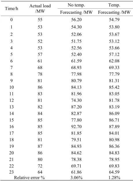
Our actual power load data and its corresponding wea- ther data come from HuaiNan electric network from April 2004 to August 2004, sampling frequency is one times each hour, sampling days is 120, so we gain 2880 (120 × 24) training data. We use trained SESVR model to forecast the load of August 10 2005. It is know that summer season influence power load more drastically an other three seasons, it is why we sample load from summer season, meanwhile, we can study whether or not weather influence and how to influence electricity load. The numerical results of short-term load forecasting were also included in following Table 1.

From Table 1 and Figure 1, we can find out our pro-

posed SESVR model is a feasible forecasting method for electric power short-term load, If we generated the train- ing samples for SESVR including the weather tempera- tures, the relative error is 1.28%, otherwise the error is 3.06%. So, the weather temperatures can upgrade fore- casting accuracies, moreover, we can

rors of night time is bigger than that of daytime. On the other hand, we find out the penalty parameter C in Algo- rithm 4.3 increases monotonously, so Algorithm 4.3 is stable, however, SVMlight _{and LIBSVM are influenced by}

penalty parameter C. In order to gain the optimal solu-tions of SVMlight _{and LIBSVM, we must tune C carefully.}

This increases the computational complexity. With re-gard to this point, Algorithm 4.3 is superior to SVMlight

and LIBSVM.

Figure 2 illustrates the tenfold numerical results and

[image:6.595.122.476.87.203.2] [image:6.595.118.482.248.358.2]

Figure 1. The electricity load forecasting results using our proposed SESVR model. Blue line, red line, and green line show the actual load, forecasting load with no temperature, and forecasting load with temperature, respectively.

Figure 2. The electricity load forecasting comparison of SESVR, SVMlight, LIBSVM. Blue line shows the actual load, read line represents the forecasting load using our proposed regression model SESVR, yellow line and green line illustrate the fore-casting loads using SVMlight and LIBSVM model, respectively.

than LIBSVM and SVMlight _model.

Table 1. The load forecasting result on 10 August 2005.

No temp. Temp.

Time/h Actual load _/MW

orecasting /MW Forecasting /MW

6. Conclusions

We opos a novel for on, SESV ich is a s oth unco ained opti on reform n of the itional linear programm ssociated n ε-I nse ive supp vector regr . We have oyed titute it f plus nuous. We have pro- rithm involving a very fast New- m to solve the SESVR that has been

lving a

F

have pr ed mulati R, wh

mo nstr mizati ulatio

trad ing a with a

nsit ort ession empl

0 55 56.20 54.79 1 53 54.30 53.80

3

o 3.

2 53 52.06 53.67 52 51.75 53.12 4 53 52.56 53.66 5 57 52.40 57.12 6 61 61.59 62.08 7 68 68.93 69.33 8 78 77.98 77.79 9 81 80.79 81.31 10 86 84.13 85.42 11 83 81.96 83.05 12 81 74.30 81.78 13 82 87.20 83.19 14 84 82.87 86.09 15 85 77.80 86.71 16 85 92.70 87.89 17 85 81.85 84.01 18 81 79.51 80.98 19 87 84.93 86.36 20 86 84.62 84.83 21 80 78.38 78.95 22 72 69.71 69.83 23

Relative err

64 r %

61.86 06%

64.59 1.28%

an en nction

function to avoid objective disconti

tropy penalty fu to subs or the

posed a new algo ton-Armijo algorith

shown convergent globally to the solution. In our algo- rithm, the penalty parameter C is creasing monotonously, the influence to SESVR performance is smaller than foregoing SVMlight _{and LIBSVM. Theoretically, we have}

given a brief convergence proof to our algorithm. In order to show the efficiency of our algorithm, we employ it to forecast an actual electricity power short- term load. The experimental results show that the pro- posed SESVR is effective and precise, and plays better performances than SVMlight _{and LIBSVR in stochastic}

time series forecasting. Moreover, an advantage of our proposed SESVR algorithm is that we only need to solve a system of linear equations iteratively instead of so

[image:6.595.56.286.421.734.2]

REFERENCES

[1] C. V. Gustavo, G. Juan and G. P. Gabriel, “On the Suitable Domain for SVM Training in Image Coding,” Journal of Machine Learning Research, Vol. 9, No. 1, 2008, pp. 49- 66.

[2] F. Chang, C. Y. Guo and X. R. Lin, “Tree Decomposition for Large-Scale SVM Problems,” Journal of Machine Learning Research, Vol. 11, No. 10, 2010, pp. 2935-2972.

[3] Y. H. Kong, W. C. Wei and W. He, “Power Quality turbance Signal Classification Using Support Vector

chine Based o ” Journal of North

Dis- Ma- n Feature Combination,

China Electric Power University, Vol. 37, No. 4, 2010, pp. 72-77.

[4] J. Zhe, “Research on Power Load Forecasting Base on Sup- port Vector Machines,” Computer Simulation, No. 8, 2010, pp. 282-285.

[5] B. Chen and P. T. Harker, “Smooth Approximations to Non- linear Complementarity Problems,” SIAM Journal of Opti- mization, Vol. 7, No. 2, 1997, pp. 403-420.

doi:10.1137/S1052623495280615

[6] C. H. Chen and O. L. Mangasarian, “Smoothing Methods for Convex Inequalities and Linear Complementarity Prob- lems,” Mathematical Programming, Vol. 71, No. 1, 1995, pp. 51-69. doi:10.1007/BF01592244

[7] C. H. Chen and O. L. Mangasarian, “A Class of Smoothing Functions for Nonlinear and Mixed Complementarity Prob- lems,” Computational Optimization and Applications, Vol. 5, No. 2, 1996, pp. 97-138. doi:10.1007/BF00249052 [8] X. Chen, L. Qi and D. Sun, “Global and Superlinear Con-

vergence of the Smoothing Newton Method and Its Appli- cation to General Box Constrained Variational Inequali- ties,” Mathematics of Computation, Vol. 67, No. 222, 1998, pp. 519-540. doi:10.1090/S0025-5718-98-00932-6 [9] Y. J. Lee and O. L. Mangasarin, “SSVM: A Smooth Support

Vector Machine for Classification,” Computational Optimi-zation and Applications, Vol. 20, No. 1, 2010, pp. 5-22. doi:10.1023/A:1011215321374

[10] Z. Q. Meng, G. G. Zhou and Y. H. Zhu, “A Smoothing Support Vector Machine Based on Exact Penalty Func-tion,” Lecture Notes in Artificial Intelligence, Vol. 3801, 2005, pp. 568-573.

[11] Y. F. Fan, D. X. Zhang and H. C. He, “Tangent Circular Arc Smooth SVM（TCA-SSVM） Research,” 2008 Congress on Image and Signal Processing, Sanya, 27-30 May 2008, pp. 646-648. doi:10.1109/CISP.2008.112

[12] Y. F. Fan, D. X. Zhang and H. C. He, “Smooth SVM

Re-“A Study on Piece-

eorgios and B. Giannakis, “Consensus-

ing Methods for search: A Polynomial-Based Approach,” The 9th Interna-tional Conference on Information and Communications Security, Singapore, 10-13 December 2007, pp. 983-988. [13] L. K. Lao, C. D. Lin, H. Peng, et al.,

wise Polynomial Smooth Approximation to the Plus Func- tion,”The 9th International Conference on Control, Auto- mation, Robotics and Vision, Singapore, 5-8 December 2006, pp. 342-347.

[14] J. Z. Xiong, T. M. Hu and G. G. Li, “A Comparative Study of Three Smooth SVM Classifiers,” Proceedings of the 6th World Congress on Intelligent Control and Automation, Dalian, 21-23 June 2006, pp. 5962-5966.

[15] P. A. Forero, A. C. G

Based Distributed Support Vector Machines,” Journal of Machine Learning Research, Vol. 11, No. 5, 2010, pp. 1663- 1707.

[16] C. H. Chen and O. L. Mangasarian, “Smooth

Convex Inequalities and Linear Complementarity Problems,” Mathematical Programming, Vol. 71, No. 1, 1995, pp. 51-69. doi:10.1007/BF01592244

[17] S. H. Peng and X. S. Li, “The Asymptotic Analysis of

chine for ε-Insensitive Regres- Quasi-Exact Penalty Function Method,” Journal of Compu- tational Mathematics, Vol. 29, No. 1, 2007, pp. 47-56. [18] Y. J. Lee, W. F. Hsieh and C. M. Huang, “ε-SSVR: A

Smooth Support Vector Ma

sion,” Knowledge and Data Engineering, Vol. 17, No. 5, 2005, pp. 678-695. doi:10.1109/TKDE.2005.77

[19] T. Joachims, “SVMlight_{,” 2010.}

http://svmlight. joachims .org

[20] C.-C. Chang and C.-J. Lin, “LIBSVM: A Library for Support Vector Machines,” 2010.

http://www.csie.ntu. edu.tw/~cjlin/libsvm [21] R. Fletcher, “Practical Method

Wiley & Sons, New York, 198

s of Optimization,” John 1.

hines,” IEEE Transac- 010, pp. 1032- [22] O. L. Mangasarian and D. R. Musicant, “Successive Over-

relaxation for Support Vector Mac tions on Neural Networks, Vol. 10, No. 5, 2 1037. doi:10.1109/72.788643

ftp://ftp.cs.wisc.edu/math-prog/tech-reports/98-18.ps [23] Y. W. Chang, C. J. Hsieh and K. W. Chang, “Training