Pricing Callable Bonds Based on Monte Carlo
Simulation Techniques
Deng Ding1, Qi Fu2*, Jacky So2 1
Faculty of Science and Technology, University of Macau, Macao, China
2
Faculty of Business Administration, University of Macau, Macao, China Email: {dding, jackyso}@umac.mo, *[email protected] Received March 20,2012; revised April 23, 2012; accepted April 30, 2012
ABSTRACT
In this paper, a Monte Carlo method, which is based on some new simulation techniques proposed recently, is presented to numerically price the callable bond with several call dates and notice under the Cox-Ingersoll-Ross (CIR) interest rate model. The corresponding algorithms are also presented to practical callable bond pricing. The numerical experi-ments show that this method works very well for callable bond under the CIR interest rate model.
Keywords: Callable Bond; Monte Carlo Simulation; CIR Model; Embedded Option Pricing
1. Introduction
A callable bond is a bond that allows the issuer to buy back the bonds from the bond holders at pre-specified prices on the pre-specified call dates. Therefore, a call-able bond is a straight bond embedded with a call of Eu-ropean option (a single call date) or Bermudan option (several call dates). However, this option is an integral part of a bond, and cannot be traded alone, and hence, its prices cannot be observed. Thus, the callable bond pric-ing must be involved in the pricpric-ing problem of the cor-responding option.
There are some different approaches for pricing call-able bonds. The first approach is based on the Black- Derman-Toy model, which was presented in [1] (2006), with the discrete simulation of binary tree. With the help of the risk-neutral valuation, the second approach is to obtain a partial differential equation (PDE) subject to appropriate boundary conditions based on the equilib-rium interest rate model. Since it is very difficult to ana-lytically solve this PDE, some different discretizations and different numerical methods have been proposed. Büttler in [2] (1995) applied finite difference method to find the evaluation of callable bonds. Büttler and Wald-vogel in [3] (1996) derived an analytic expression for the Green's function of the corresponding PDE for certain specific interest rate models, and developed a semi-ana- lytic method for pricing callable bonds with notice. As the further development, the finite volume method was used by D’Halluim et al. in [4] (2001), and the finite ele-ment method was considered by Farto and Vázquez in [5]
(2005) for the numerically pricing callable bonds with notice. Recently, a dynamic programming approach was proposed by Ben-Ameur et al. in [6] (2007) for numeri-cally pricing options embedded in bonds. In this dynamic programming approach they used finite difference method and solved the Green’s function by conditional distribu-tions and expectadistribu-tions with piecewise-linear approxima-tion.
Meanwhile, in the last decade, many new numerical schemes for simulations of interest rate models, espe-cially, the Cox-Ingersoll-Ross (CIR) interest rate model, have been proposed. For instance, the balanced implicit method (BIM) was proposed by Milstein et al. in [7] (1998), the balanced Milstein method (BMM) was de-veloped by Kahl and Schurz in [8] (2006). Also, the ex-act transition distribution method (ETD) is considered to simulate the square-root diffusions (e.g. see [9]). Re-cently, a new splitting-step scheme was presented by Ding and Chao in [10] (2009). In this paper, based on these new simulation techniques we present a Monte Carlo method to numerically price the Bermudan-type callable bond with notice.
This paper is structured as follows. After this introduc-tion, the interest rate models are reviewed, and several numerical simulation techniques are surveyed in Section 2. Then, based on these simulation techniques, an effi-cient Monte Carlo method is presented to price the call-able bond with several call dates and notice under the CIR interest rate model in Section 3. The corresponding algorithms are presented in this section. Finally, numeri-cal experiments for a practinumeri-cal numeri-callable bond with 10 numeri-call dates and 2 months notice are provided in Section 4. The
*
numerical results of these experiments are also presented in this section, as well as some useful conclusions.
2. Simulations of Interest Rate Models
Pricing financial derivatives depends on the description of the dynamic process of underlying assets. Since the underlying asset of callable bond is the interest rate, we focus on the mathematical models for the interest rate. These models can be divided as single factor models and multiple factor models by the number of status variables.
The first well-known single factor model was pro-posed by Vasicek in [11] (1977). In this model, the in-terest rate is give by the stochastic differential equation (SDE):
r t
dr t r t dtdW t ,
where , and are all strictly positive constants, and W t
is a standard Brownian motion. In detail, represents the speed at which r t
reverts back to the long-term mean , while is the local volatility of short-term interest rates. The Ornstein-Uhlenbeck pro- cess is employed in this model for its key feature as the mean-reverting structure.The Vasicek’s model has two significant failings. First, the interest rate can become negative; Second, empirical evidence suggests that the volatility of is not con-stant as
r t , but is an increasing function of r t
in-stead. The first single factor model that possesses non- negative interest rate is the CIR model, which was pro-posed by Cox, Ingersoll and Ross in [12] (1985). In this CIR model the interest rate r t
follows the following SDE:
dr t r t dt r t dW t . (1) This model embodies the feature that the volatility is an increasing function of r t
. In this paper we focus on this model.Although the application of the Yamada’s condition reveals that the SDE (1) has a unique non-negative solu-tion r t
for any given initial value r
0 0 is dif-ficult to find an explicit formula for this solution. Thus, many practical applications lead to the numerical simula-tion of the CIR model. However, this involves two pro- blems: The first one is that the numerical simulation would yield negative value in the general discretization of SDE (1); The second one is that, since the diffusion coefficient is not globally Lipschizian, the convergence of the general discretization for SDE (1) is not guaran-teed.
, itments in Section 4.
be a positive integer. In the fo
In the last decade, many efficient new numerical schemes have been proposed for the CIR model (1) with positivity preservation. In the following, we survey these schemes, which are employed in the numerical
experi-Let T > 0 and let N
llowing we denote T N, and set t00 and k
t k for each k1,,N , i.e. t0 1 tN is
of
t a
partition
0,T . We enote eachk. We assum at 1, ,
also d rk r t
k fore th N are N dent ran-
m variables having on standard normal distri-bution.
The b
indepen
do a comm
alanced implicit method (BIM) was proposed by Milstein et al. in [7]. The discretisation of the CIR model (1) by the BIM is given by
1 1 1
1 1
,
k k k k
k k k
k
r
r r r
r r r
(2)
for each k1,,N, where
xy
is called the control function, and here it is given b
rk 1 k C (3)
with C rk1 for rk1 ; and C else-
where. Here is ossible bu
ein method (BMM) was developed by
selecte all as p t
halt-ing the computation. The balanced Milst
d as sm
Kahl and Schurz in [8]. For CIR model (1) the BMM scheme is given by
2 2
1 1
1
1
1 4
,
k k k k k
k k
r r r
r r
(4) for each k1,,N
for the CIR
. BIM and BMM schemes preserve IR m
positivity model (1) as tends to zero. In the book [9], an algorithm for simulation of the C odel (1) by the exact transition distribution (ETD) me-thod is given in the following.
The CIR model (1) with d 4 2: Case 1:
for
1
d
0, , 1
k N
1
2 1 tk tk 4
c e
tk1 tk
k
r e c
generate Z N
0,12
X
generate d1
21 k
r c Z X
end
Case 2: d 1 for k0,,N1
1
2 1 tk tk 4
c e
tk1 tk
k
r e c
generate N Positon
2
2
generate X d2N
X
1 k
r c
The adv e o vation
antag f this algorithm is the strict positivity p , comparing the conditional preservations of the two methods above. Howeve ETD method suf-fers so great cost of computational time, and it also seems to be relatively unsuitable in our numerical ex-periments.
Recently, an efficient splitting-step scheme for the CIR ) was pro ed by Ding and Chao in [10]. This new scheme, which is called the DC scheme here, is given as
reser
r, the
model (1 pos
2
2
1
1 1
1
2 k 4
r r e
(5) for each . This scheme preserves the posi-
tivity fo the case: , and it
take al time in p BIM and
BM s.
3. The Monte Carlo Method
W
1
e
k k
1, ,
k N
r the simulatio putation
n in 4 2
arison to
s less com com
M scheme
e consider a Bermudan callable bond which has mn
pre-specified coupon dates:
0 1 m J n J 1 J
t t t t t t ,
where the bond may be redeemed at the last n dates (call dates): J n , , J1
d between each notice date and corresponding call date is denoted as
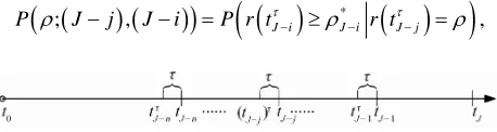
t t . As in Figure 1, the notice pe-rio
. For convenience, tJ j tJ j
is denoted the (n – j + 1)th notice date for each
, ,1
jn . In general, tes is one year,
the time period and the annual
betw n two coupon yment
ee pa coupon da
is denoted as . At the call date tJj, the call (o strike) r
price is defined as XJj, jn,,1.
Let E and P
denote the conditionalwhen
ex- pectation and conditional probability under the risk-neu- tral probability measure P. For two dates
0 i j J
t t t t , we define the discount factor over the time period t ti, j r t
i :
; ,
exp
j
d
i i
t
E i j E t r s s r t
,where r t
is the instantan
eous interest rate with the initial value r t
0 r0. For two notice dates tJ j tJ i
,
we also denote:
*
; , J i J i J j
[image:3.595.58.287.649.710.2]P Jj Ji P r t r t ,
Figure 1. The call dates and the corresponding notice dates of Bermuda ca ble bond.
where *
lla
J i
is the break ven (or critical) interest rate at -e the notice date tJ i
. If the interest rate r t
J i at the
notice date tJ i
is less than the break-even interest rate *
J i
the issuer should call the bond at the call date tJ i ,
otherwise the debt (the callable bond in aspect of the be hold.
issuer) should
callabl embedded a Bermudan op-tion, its value is computed recursively by the backward induction. At the first notice date
Since the e bond is
1
J
t , under the condi-tion: r t
J 1
, if the bond is not called, its value is
given b
1 ; 1 1 ; 1
y
uncall
, ,
; 1 , 1 ,
K J J E J J
E J J
where
J1
represents the date tJ 1
; if the bond is
called, the value is given by
; 1 , ; 1 , 1
K J J X E J J
1 1
call J
The issuer of the bon
. d should minimizes his out-standing debt. If the price of the callable bo greater than the time value of the call price including the coupon payment, he will call the bond to meet the requirement of the optimal call policy. That means he will choose the minimum value between uncall and call values, i.e., the value of the bond at the
nd is
date tJ 1
should be given by
1
; 1 ,
min 1 , , ; 1 , .
K J J
K J J K J J
1
1
uncall call
;
To solve this optimal problem, we can consider the following equation for the variable :
1 ; 1 , 1 ; 1 ,
K J J K J J
uncall call
Then, the root of this equa *
. (6) tion is the break-even in- terest rate J1. There are some different methods to find this ro the CIR model (1), the paper [3] giv a formula for the root:
ot. For es
1
* 1
1 1
1
ln 1
J J
X f
g g f
, (7)
where 1 tJ tJ1, and functions f and g are
de-fined by
2
2
2
2
2 1
t
t
e f t
e
,
2 1
2 1
t
t
e g t
e
with 222 and the sum of the risk premium
, which is a parameter. Also, we can approximate the ot
ro *J1 rent val
by computing uncall and call values for the
ffe ues of
di via the Monte Carlo simula
Now, the value of the bond at the notice date tion.
1
J
t is
gi 1 , (8)
sets and respectively.
We then consider the bond value at the se notice date . Under the condition:
ven by
1
K ; J 1 , J
* 1 1 uncall * 1 call; 1 , 1
; 1 , 1
J
J
K J J
K J J
where 1
and 1
*J1 are indictors of * 1 J
*
1 : J
: *J1
cond 2
J
t r t
J 2
, if the bond
is uncalled, its value is give by
1 1 1 2; 1 ,
exp J d
J
t
J t
J J
r s s r t
2 uncall; 2 ,
; 2 , 2 .
K J J
E K r t
E J J
2 J
Combining the expression (9) we have
(9)
2 uncall 1; 2 , 1 ; 2 ,
; 2 , 1 ; 2 , 1
2 , 1
1 ; 1
J
; 2 ,
; 2 , 2 .
K J J E J
E J J P J J
X E J
P J J J J (10)
E J J
On the other hand, if the bond
is called, under the giv-en condition: r t
J 2
, the value is given by
(11) Therefore, the bond value at the second no
is given by
2 2 , (12) where
2 2 call; 2 , J ; 2 , 2
K J J X E J J ,
tice date 2
J
t
2 * * 2 call; 2 ,
; 2 , 1
J
J
K J J
K J J
2 uncall; 2 , 1
K J J
* 2
J
ce date t
is the break-even interest rate at the second
noti J 2
, which can be found as the first break-
even interest rate *J1. ly, we can
Con obtain the values of callable
bond at the jth notice date tinuous
J j
t
as
j
(13)
where
*
uncall
; ,
; , 1
j
j J
K J j J
K J j J
*
call; , 1 ,
j J j
K J j J
* J j
ce date
is the break-even interest rate at the jth noti tJ 1
.
tly,
Con we get the price of the callable b the prese
sequen ond at
nt date t00 with the initial interest rate
t0 r0r :
0 0 0 0 0 1 ; 0, ; ,; 0, ; 0, .
n J n
m
i
K r J
E K r t J n J r t r
E r J n E r i
(14) by apNow, plying the simulation technique to the in-terest rate r t
and using the Monte Carlo method to approximate the corresponding integrals E
; ,i j
and the corresponding probabilities P
;
Jj
, Ji
, we can obtain a numerical approximation of the price
0; 0,
K r J .
4. Numerical Experiments
In this section, we do numerical experiments vi
thods to price a callable bond issued by the Swiss Con-federation with an annual coupon of 4.25%. Here is
er 2
a our
me-0
t
Decemb 3, 1991, and tJ is December 31, 2012. The
protection p riod is 10 years until year 2002. The notice pe
e
riod is two months. And the call prices are
1 5 1
J J
X X , XJ61.005, XJ71.01,
1.015
8 J
X , XJ91.02 and XJ101.025, resp ec-From [3], the model parameters for the CIR model are tively.
0.54958046
, 0.38757496, 0.0348468515.
80589
The initial interest rate r00.07522 , and th
k-even interest rates
0.0179273733,
8817260, e price of straight bond i
are *J10.03 * 3 0.009978 J [3]
s 0.8114. The brea
71564, J*2
92562, *J4 0.004
388
*
5 0.0015784739
J and
* *
6 10 0
tion (6 fore we use the res -even interest rates
J J
, which
Table 1. Numerical results for four methodsa.
DC ETD
Nb = 240 BIM BMM
Callable bondc 0.8814 0.7967 0.8089 0.8575
Call optiond –0.07 0.0147 0.0025 –0.0461
[image:5.595.56.287.197.256.2]Errore 8.33E–2 1.40E–3 1.08E–2 5.94E–2
Table 2. Numerical results for different Ns via BMM me- thoda.
40 0 0
Nb 2 48 96
Callable bond 0.c 7967 0.8009 0.7974
Call option 0.0147 0.0105 0.014
e 40E E–03
d
[image:5.595.55.288.284.344.2]Error 1. –03 2.80 7.00E–04
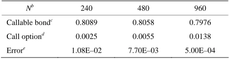
Table 3. Numerical results for different Ns via DC methoda.
0
Nb 240 480 96
Callable bondc 0.8089 0.8058 0.7976
Call optiond 0.0025 0.0055 0.0138
Errore 1.08E–02 7.70E–03 5.00E–04
a
All prices of callable bond are computed by the ave- rage over 50,000 simulating
b
paths.
N i he
si-mula nterest rate.
c
es for allab d are ed
s its e 1 resu
s of be ll all e
v
Error is the absolute difference between callable bond s 1-3 give the price of this callable bond via dif-ferent simulation methods. All results in the num experi s show t MM and schemes are more
e the Mo rlo met rks
v r prici ble bon
5. Acknowledgements
of Macau for supporting their work G136(Y1-L2)-
FST1 D, SRF02 10S/11T/ /FBA).
REFERENCES
s the number of time-discretized points in t tion of i
All figur the c le bon round to four ignificant dig from th 5-digit lts.
d
All price the em dded ca option per fac alue.
e
price and 0.7981, which is given in [3]. Table
erical
ment hat B DC
fficient than others. And nte Ca hod wo ery well fo ng calla ds.
The authors thank the Research Committee of University (MYR
SYC
1-D
3/09-[1] Z. L. Zheng and C. F. Kang, “Pricing and Hedging of Chinese Interest Rate Derivatives,” Peking University Press, Beijing, 2006.
[2] H.-J. Buttler, “Evaluation of Callable Bonds: Finite Dif-ference Methods, Stability and Accuracy,” The Economic Journal, Vol. 105, No. 429, 1995, pp. 374-384.
doi:10.2307/2235497
[3] H.-J. Buttler and J. Waldvogel, “Pricing Callable Bonds ction,” Mathematical Finance,
. 8, No. 1, 2001, pp. 49-77. doi:10.1080/13504860110046885
by Means of Green’s Fun Vol. 6, No. 1, 1996, pp. 53-88.
[4] Y. D’Halluin, P. A. Forsyth, K. R. Vetzal and G. Labahn, “A Numerical PDE Approach for Pricing Callable Bonds,” Applied Mathematical Finance, Vol
[5] J. Farto and al Techniques for
Pricing Callab Applied Mathema- C. V’azquez, “Numeric
le Bonds with Notice,”
tics and Computation, Vol. 161, No. 3, 2005, pp. 989- 1013. doi:10.1016/j.amc.2003.12.079
[6] H. Ben-Ameur, M. Breton, L. Karoui and P. L’Ecuyer,
.
6.06.007
“A Dynamic Programming Approach for Pricing Options Embedded in Bonds,” Journal of Economic Dynamics and Control, Vol. 31, No. 7, 2007, pp. 2212-2233
doi:10.1016/j.jedc.200
ol. 35, No. 3, 1998, pp. [7] G. N. Milstein, E. Platen and H. Schurz, “Balanced
Im-plicit Methods for Stiff Stochastic Systems,” SIAM Jour-nal on Numerical AJour-nalysis, V
1010-1019. doi:10.1137/S0036142994273525
[8] C. Kahl and H. Schurz, “Balanced Milstein Methods for Ordinary SDEs,” Monte Carlo Methods and Applications, Vol. 12, No. 2, 2006, pp. 143-170.
doi:10.1515/156939606777488842
[9] P. Glasserman, “Monte Carlo Methods in Financial En-gineering,” 2nd Edition, Springer, New York, 2004. [10] D. Ding and C. I. Chao, “An Efficient Numerical Scheme
Term Economices, Vol. 5, No. for Simulation of Mean-Reverting Square-Root Diffu-sions,” Journal of Numerical Mathematics and Stochas-tics, Vol. 1, No. 1, 2009, pp. 45-55.
[11] O. Vasicek, “An Equilibrium Characteriaztion of the Structure,” Journal of Financial
2, 1977, pp. 177-188.
doi:10.1016/0304-405X(77)90016-2