Evaluation of Atmospheric Correction Algorithms for Landsat 8 OLI and MODIS Aqua to Study Sediment Dynamics in the Northern Gulf of Mexico

ISSN Online: 2169-2688 ISSN Print: 2169-267X

DOI: 10.4236/ars.2018.72008 Jun. 22, 2018 101 Advances in Remote Sensing

Evaluation of Atmospheric Correction

Algorithms for Landsat-8 OLI and

MODIS-Aqua to Study Sediment Dynamics

in the Northern Gulf of Mexico

Nazanin Chaichitehrani

_{, Erin Lee Hestir}

_{, Chunyan Li}

1_{Department of Oceanography & Coastal Sciences, Louisiana State University, Baton Rouge, USA} 2_{School of Engineering, University of California, Merced, USA}

Abstract

Suspended particulate matter (SPM) is regarded as an energy source and a water quality indicator in coastal and marine ecosystems. To estimate SPM from ocean color sensors and land observing satellites, an accurate and robust atmospheric correction must be done. We evaluated the capabilities of ocean color and land observing satellite for estimation of SPM concentrations over Louisiana continental shelf in the northern Gulf of Mexico, using the Opera-tional Land Imager (OLI) on Landsat-8, and Moderate Resolution Imaging Spectroradiometer (MODIS) on Aqua. In high turbidity waters, the traditional atmospheric correction algorithms based on near-infrared (NIR) bands unde-restimate SPM concentrations due to the inaccurate removal of the aerosol contribution to the top of atmosphere signals. Therefore, atmospheric correc-tion in high turbidity waters is a challenge. Four atmospheric correccorrec-tion algo-rithms were implemented on remote sensing reflectance (Rrs) values to select suitable atmospheric correction algorithms for each sensor in our study area. We evaluated short-wave infrared (SWIR) and NIR atmospheric correction algorithms on Rrs products from Landsat-8 OLI and Management Unit of the North Sea Mathematical Models (MUMM) and SWIR.NIR atmospheric cor-rection algorithms on Rrs products from MODIS-Aqua. SPM was retrieved from a band-ratio SPM-retrieval algorithm for each sensor. Our results indi-cated that SWIR atmospheric correction algorithm was the suitable algorithm for Landsat-8 OLI and SWIR.NIR atmospheric correction algorithm outper-formed MUMM algorithm for MODIS.

Keywords

Suspended Particulate Matter, Remote Sensing, Atmospheric Correction

How to cite this paper: Chaichitehrani, N., Hestir, E.L. and Li, C.Y. (2018) Evaluation of Atmospheric Correction Algorithms for Landsat-8 OLI and MODIS-Aqua to Study Sediment Dynamics in the Northern Gulf of Mexico. Advances in Remote Sensing, 7, 101-124.

https://doi.org/10.4236/ars.2018.72008

Received: April 21, 2018 Accepted: June 19, 2018 Published: June 22, 2018

Copyright © 2018 by authors and Scientific Research Publishing Inc. This work is licensed under the Creative Commons Attribution International License (CC BY 4.0).

http://creativecommons.org/licenses/by/4.0/

DOI: 10.4236/ars.2018.72008 102 Advances in Remote Sensing Algorithms, River Plume

1. Introduction

Suspended particulate matter (SPM) plays a major role in the biological and ecological status of inland, coastal, and shelf waters, and can cause detrimental effects on marine ecosystems [1] [2] [3] and has a strong influence on the phy-toplankton productivity and abundance by changing photosynthetically active radiation (PAR) and euphotic depth [4]. To understand the influence of SPM on water quality impairment and nutrient availability in coastal waters and river plumes, it is imperative to study the temporal and spatial dynamics of SPM. The traditional method of monitoring SPM using ship and platform measurements is limited in spatial coverage, and it can be difficult to maintain regular monitoring programs for time-series assessments. However, with the advent of satellite-based sensors and computer simulation packages, some studies on SPM dynamics with a high spatial and temporal resolution have been done [5] [6] [7]. A well-cali- brated and validated sediment transport model along with a reliable satel-lite-derived SPM data can provide spatially continuous near-surface maps of SPM. Among ocean color sensors and land imagers, the capability of Landsat-8, Operational Land Imager (OLI) and Aqua, Moderate Resolution Imaging Spec-troradiometer (MODIS) to estimate SPM in coastal waters have been proven [8] [9] [10]. Landsat-8 was launched on February 11, 2013 and started operating on May 30, 2013. It has 11 spectral bands (433 - 12,500 nm), spatial resolutions of 30 m and 15 m in the panchromatic band, and a revisit time of 16 days. The high signal-to-noise ratio (SNR), the 12-bit quantization combined with 30 m spatial resolution of the Landsat-8 OLI enhance our ability to monitor SPM dynamics in coastal waters [11] [12]. Landsat-8 OLI spatial resolution is sufficient to re-solve SPM plume and to provide a map of the well-defined turbidity plume from the Mississippi River (Figure 1). However, with a designed revisit time of 16-days and an effective revisit time of c.a. seasonal when cloud cover is taken into account [13], Landsat’s temporal resolution is highly limited for studying the SPM dynamics over regions with the high sediment dynamics regime.

DOI: 10.4236/ars.2018.72008 103 Advances in Remote Sensing Figure 1. Rayleigh-corrected Landsat-8 OLI image over the Mississippi River plume, coastal water and Lousiana continental shelf waters on 23 April 2016 representing high turbidity waters around the Mississippi River’ passes and coastal waters as well as the dispersion of sediment-rich water to offshore waters. Box 1, box 2 and box 3 represent high, moderate and low turbidity water.

Mississippi River plume. Thus, to study sediment dynamics Landsat-8 OLI and MODIS-Aqua should be used in tandem in our study region partiality during extreme meteorological events. SPM is retrieved from satellite data by relating its concentration to apparent optical properties (AOPs) (e.g., empirical algorithms) and inherent optical properties (IOPs) (e.g., semi-analytical and analytical algo-rithms) in high and in low to moderate turbid waters (Case-II and Case-I, re-spectively) [8] [21] [22] [23] [24].

DOI: 10.4236/ars.2018.72008 104 Advances in Remote Sensing negligible, and any measured signal is due to aerosol scattering [30] [31]. Hence, NIR atmospheric correction algorithms for SPM retrieval in high turbidity wa-ters can lead to an overestimation of aerosol reflectance and an underestimation of SPM concentration [32]. While it has been shown that short-wave infrared (SWIR) atmospheric correction algorithms can perform well in high turbid coastal waters [33] [34]. In recognition of difficulties for selecting the most effec-tive atmospheric correction methods in high turbidity water, developing of at-mospheric correction models based on the combination of NIR and SWIR bands or two SWIR bands has gained increased attention [12] [34] [35] [36] [37]. Ody

et al. [10] evaluated NIR and SWIR atmospheric correction for Landsat-8 and

Management Unit of the North Sea Mathematical Models (MUMM) and NIR-SWIR for MODIS attempting to study the sediment dynamics in Rhone River plume.

The main objective of this paper is to evaluate different atmospheric correc-tion methods for three study areas covering high to low turbidity waters in the northern Gulf of Mexico and an aim to develop SPM maps that can be used to evaluate sediment transport models was made. Accurate maps of SPM can also be used as indicators of coastal dynamics to improve our understanding of coastal zone hydrodynamics and to help prioritize sampling locations and field surveying times. Furthermore, daily MODIS-derived SPM can be used as an ini-tial condition input in sediment transport and ecosystem models.

To the best of our knowledge, no study has yet been undertaken to test or evaluate atmospheric correction algorithms performance using Landsat-8 OLI and MODIS-Aqua for retrieval of SPM in the northern Gulf of Mexico coastal and shelf waters.

2. Methods

The overarching goal of this study is to estimate SPM concentration using Landsat-8 OLI and MODIS-Aqua. To achieve this goal, the following steps should be performed:

1) Identify the most appropriate and suitable atmospheric correction methods across high- to low-turbidity waters.

2) Apply a standard SPM retrieval algorithm [23] across all corrected datasets. 3) Compare retrieved SPM concentration with in situ-measured SPM concen-tration.

2.1. Study Area

DOI: 10.4236/ars.2018.72008 105 Advances in Remote Sensing primary productivity and fishery activities in the northern Gulf of Mexico [14] [42] [43] [44].

The SPM dynamics around the Mississippi River delta is optically complex and variable in time and space. Sediment resuspension as a geomorphic response to extreme weather events (e.g., hurricanes and cold fronts) contributes to the turbidity and the complexity of the Mississippi River delta and coastal waters in the northern Gulf of Mexico. Figure 1 presents a Rayleigh-corrected RGB Landsat-8 OLI image over the Mississippi River plume on 23 April 2016 showing turbid coastal waters with high sediment concentration (yellow-brown) around the Mississippi River passes, as well as the extension of sediment-laden waters to the Lousiana continental shelf.

This true color satellite image shows a distinct dispersal pattern of turbidity into the Gulf of Mexico and coastal areas around the Mississippi River passes. The Mississippi River tends to direct the plume to the northwest during fall and winter and to the east during spring and summer [5] [7] [45] [46] [47] [48] [49]. Wind-generated currents and waves are the most important geological agents controlling sediment dynamics over the Louisiana continental shelf [5].

To investigate the performance of atmospheric correction algorithms and to select the most appropriate approaches in our study area, our study area was di-vided into three regions ranging from high-to-low turbidity (Figure 1).

These three regions were selected based on the distance from the Mississippi River passes (e.g., Southwest Pass) as well as assessing true color images obtained from different time periods. Box 1 is in the vicinity of the Mississippi River passes and encompasses the high turbidity water. This region is highly influ-enced by the Mississippi River sediment plume. Box 2 encloses the moderate turbid water, and this region is relatively far from the Mississippi River passes. This region is influenced by tidal-induced transport of suspended sediment from the Barataria Bay (see Figure 2 for location). Box 3 surrounds the low turbid water, which is far from the Mississippi River plume (Figure 1).

2.2. Landsat-8 OLI Data Collection and Atmospheric Correction

In this study, the remote sensing reflectance (Rrs) at 443 nm (coastal/aerosol), 483 nm (blue), 560 nm (green), 655 nm (red), 864 nm (NIR) and two SWIR bands at 1601 nm and 2380 nm were used in atmospheric correction algorithms and the subsequent SPM retrieval algorithm. Two atmospheric correction approaches were applied to the Landsat-8 OLI data, ACOLITE-NIR and ACOLITE-SWIR.

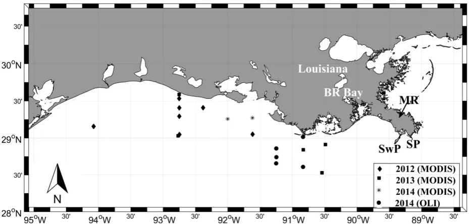
DOI: 10.4236/ars.2018.72008 106 Advances in Remote Sensing Figure 2. Map of our study area and the location of stations used to perform the match-ups between Landsat-8 OLI-, MODIS-derived SPM concentrations and in situ SPM concentrations (see Table 1 for detail). The geographic location of the Barataria Bay, the Mississippi River, Southwest Pass, and South Pass labeled as BR Bay, MR, SwP, and SP, respectively.

Table 1. Summary of data sets used in match-up comparisons between in situ and OLI-, MODIS-derived SPM.

Date Satellite Reference

25-27 July 2012 MODIS-Aqua [54]

8 March 2013 MODIS-Aqua [55]

13 June 2013 MODIS-Aqua [55]

23 July 2013 MODIS-Aqua [55]

13-14 September 2013 MODIS-Aqua [53]

30 July 2014 MODIS-Aqua and Landsat-8 OLI [50]

data was obtained on 30 July 2014 (Table 1). Table 2 provides Landsat-8 OLI spectral bands, SNR and corresponding spatial resolution used in this study.

The ACOLITE (version 20170718.0) software package

(https://odnature.naturalsciences.be/remsem/software-and-data/acolite) was used to obtain atmospherically corrected remote sensing reflectance products [9] [12]. ACOLITE is an atmospheric correction and processor for the Landsat-8, and Sentinel-2A (S2A) MultiSpectral Imager (MSI) developed at the Royal Belgian Institute of Natural Science (RBINS).

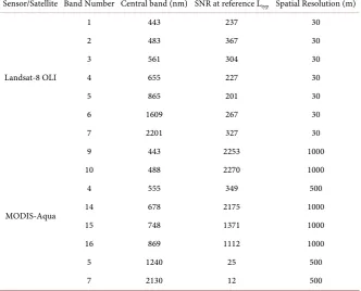
DOI: 10.4236/ars.2018.72008 107 Advances in Remote Sensing Table 2. Landsat-8 OLI and MODIS-Aqua’s band specifications used in this study.

Sensor/Satellite Band Number Central band (nm) SNR at reference Ltyp Spatial Resolution (m)

Landsat-8 OLI

1 443 237 30

2 483 367 30

3 561 304 30

4 655 227 30

5 865 201 30

6 1609 267 30

7 2201 327 30

MODIS-Aqua

9 443 2253 1000

10 488 2270 1000

4 555 349 500

14 678 2175 1000

15 748 1371 1000

16 869 1112 1000

5 1240 25 500

7 2130 12 500

2.3. MODIS-Aqua Data Collection and Atmospheric Correction

MODIS-Aqua Level-1A data were downloaded from NASA Ocean Color website (https://oceancolor.gsfc.nasa.gov) (Table 1). The Level-1 A data were processed and was upgraded to Level 1B using SeaDAS (version 7.4.). The SeaDAS package has been developed and distributed by NASA’s Ocean Biology Processing Group. Level-2 remote sensing reflectance at 443, 488, 555, and 678 nm were generated by applying MUMM [32] and SWIR.NIR atmospheric correction al-gorithms (Wang and Shi 2007; Wang, Son, and Shi 2009) [34] [37] using the l2gen function.

The MUMM correction used two MODIS NIR bands at 748 nm and 869 nm. The SWIR.NIR correction was applied using two MODIS NIR bands at 748 nm and 869 nm and two SWIR bands at 1240 nm and 2130 nm. All Rrs products were generated at a resolution of 1 km. Table 2 summarises the MODIS-Aqua bands used in this study.

2.4. SPM Retrieval Algorithm

al-DOI: 10.4236/ars.2018.72008 108 Advances in Remote Sensing gorithm performed better, and the errors were minimized compared to the pre-vious single-band SPM retrieval algorithm in the northern Gulf of Mexico [8].

In addition, the use of band (670 nm) closest to NIR bands makes this algo-rithm more robust than other visible single-band algoalgo-rithms [8]. This algorithm is the only available band-ratio algorithm designed to estimate SPM concentra-tion (mg.l−1_{) from SeaWIFS in the northern Gulf of Mexico, but in this study the} lack of in situ Rrs led us to adjust and modify this algorithm based on closest available bands in Landsat-8 OLI and MODIS-Aqua. Remote sensing reflectance products were replaced with the closest available wavelengths in Landsat-8 OLI (560 nm and 655 nm) and MODIS-Aqua (555 nm and 678 nm). The algorithm was applied to the atmospherically corrected remote sensing reflectance prod-ucts from Landsat-8 OLI and MODIS-Aqua.

1.11

670 17.783

555

Rrs SPM

Rrs

 

= _{ }

 

2.5.

In Situ

SPM Measurements

To validate Landsat-8 OLI-derived SPM concentrations, in situ SPM concentra-tions (Figure 2, Table 1) measured on 30 July 2014 were used [50]. The time difference of ±3 hr between SPM measurements and Landsat-8 OLI overpass was considered [52]. MODIS-estimated SPM concentrations were validated us-ing the SPM concentrations measurements provided by NASA SeaWiFS Bio- optical Archive and Storage System (SeaBASS) [53] and by NOAA National Centers for Environmental Information (NCEI) [50] [54] [55]. The in situ SPM dataset collected in July 2012, March, June, July, September 2013, and July 2014 matched-up with MODIS-derived SPM concentrations (Figure 2, Table 1). The time difference between SPM measurements and MODIS-Aqua overpasses used in the validation was constrained to ±3 hr [52].

3. Results and Discussion

3.1. Landsat-8 OLI

3.1.1. Comparison of Atmospheric Correction Approaches

DOI: 10.4236/ars.2018.72008 109 Advances in Remote Sensing

100 2

SWIR NIR SWIR NIR

− ×

+ (2)

3 1

2

Q Q

SIRQ= −

where Q1 is the 25th percentile and Q3 is the 75th percentile.

The 5th _{percentile of the SWIR- and NIR-corrected Rrs at 483 nm were} respec-tively ~0.0110 sr−1 _{and ~0.010 sr}−1 _{and the 95}th _{percentile of the SWIR- and} NIR-corrected Rrs were respectively ~0.0171 sr−1 _{and ~0.0140 sr}−1 _{in high-turbidity} waters (box 1) followed by 20.5% difference (Table 3).

The percentage difference decreased to 16.6 in box 3 at 483 nm. In the red band (655 nm), the percentage difference between Rrs corrected by SWIR and NIR approaches was 33.18% in high turbidity waters and 15.0% in moderately turbid waters. In box 1, The NIR atmospheric correction algorithm retrieved negative or NAN Rrs values that were not included in match-ups.

The SWIR-corrected Rrs products had higher values compared to the NIR-corrected Rrs products. The maximum percentage difference (33.18%) was observed in box 1 (high turbid waters) at 655 nm. The computed percentage dif-ferences suggested that the difference between the SWIR- and NIR-corrected Rrs at each wavelength increased as the turbidity increased.

The observed percentage difference between SWIR-and NIR-corrected Rrs values in high turbidity water could be due to the fact that the NIR-correction is only adapted to low to moderately turbid waters. The atmospherically corrected Rrs products using SWIR and NIR approaches were plotted and color-coded based on the distance (km) from the Southwest Pass (see Figure 2 for location)

Table 3. 5th _{and 95}th _{percentile for Landsat-8 OLI-retrieved Rrs (sr}−1_{) products on 23 April 2016 processed by NIR and SWIR} at-mospheric correction algorithms, the percentage difference, median NIR to SWIR ratio, and SIQR in box 1, 2 and 3.

Band Box _{SWIR approach} 5th percentile _{SWIR approach} 95th percentile _{NIR approach} 5th percentile 95_{NIR approach} th percentile Percentage _{Difference Ratio (SIQR)} Median

443 nm

1 0.0066 0.0117 0.0052 0.0097 14.50 0.930 (±0.110) 2 0.0035 0.0058 0.0032 0.0056 12.80 0.928 (±0.102) 3 0.0024 0.0039 0.0019 0.0033 9.09 0.917 (±0.058)

483 nm

1 0.0110 0.0171 0.0100 0.0140 20.49 0.959 (±0.067) 2 0.0047 0.0072 0.0046 0.0071 17.28 0.953 (±0.069) 3 0.0034 0.0048 0.0031 0.0043 16.60 0.945 (±0.041)

561 nm

1 0.0185 0.0265 0.0184 0.0240 14.73 0.978 (±0.039) 2 0.0046 0.0079 0.0044 0.0076 14.06 0.969 (±0.057) 3 0.0026 0.0040 0.0024 0.0036 13.20 0.934 (±0.057)

655 nm

DOI: 10.4236/ars.2018.72008 110 Advances in Remote Sensing (28˚54'18"N 89˚25'42"W) (Figure 3, left panel) and SPM concentrations (mg∙l−1₎ (Figure 3, right panel). The hydrodynamics around the Mississippi River plume is very complex, and sediment flux from the River is not restricted to any specif-ic outlet. Figure 3 left panel shows the Rrs signal increased as the distance from the Southwest Pass decreased and the SPM concentrations increased. The linear relationship between corrected Rrs products was observed in band 1 through 4, while as the turbidity started increasing (moving toward box 1) the linear rela-tionship failed as the data deviated from 1:1. Figures 3(a)-(d) shows that remote sensing reflectance values at 443 nm and 483 nm increased as the water became more turbid and the data were strikingly pulled down from 1:1. Furthermore, Figures 3(a)-(d) depicts that the short wavelengths (443 nm: aerosol band and 483 nm: blue bands) are highly sensitive to increase in SPM concentration (mg∙l−1_{) compared to green (561 nm) and red (655 nm) bands.}

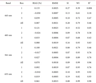
The best agreement was obtained between SWIR-and NIR-corrected Rrs at 655 nm (slope = 0.92, R2 _{= 0.98), and the lowest agreement was observed at} be-tween SWIR and NIR corrected Rrs at 443 nm (slope = 0.53 and R2 _{= 0.46) for} all data points located in three boxes (Figure 3(a) and Figure 3(c)). Table 4 presents computed statistical parameters including BIAS, root mean square er-ror (RMSE), scatter index (SI), Willmott Index (WI) (Equation (4)) and the coefficient of determination (R2_{) for Landsat-8 OLI Rrs products processed by} NIR and SWIR atmospheric correction algorithms. The Willmott Index pre-sented by [56] as:

( ) ( )

( )

( )

y j x j

d

y j y x j x

= = −     = −  − + −   

∑

∑

where x(j) are measured values, y(j) are simulated values, and x and y

represent the mean values of measurement and simulation, respectively. Index values vary between 0 for poor agreement and 1 for a perfect match. As turbidity increases, the agreement between corrected Rrs products using NIR and SWIR algorithms decreased (Table 4). The non-linear relationship was pronounced for Rrs values larger than 0.009 sr−1 _{at 443 nm and greater than 0.015 sr}−1 _{at 483 nm} where the NIR algorithm retrieved lower Rrs values than the SWIR algorithm (Figures 3(a)-(d)). The linear relationship between SWIR and NIR corrected Rrs at 655 nm observed for the values of Rrs smaller than ~0.027 sr−1 _{and the} SPM concentrations lower than ~20 mg∙l−1 _{in low and moderate turbid water} (located at a distance greater than 25 km from the Southwest Pass) (Figure 3(g) and Figure 3(h)). At 561 nm and 655 nm, nonlinearity was observed for values larger than 0.025 sr−1 _{and 0.028 sr}−1_{, respectively.}

The observed non-linearity with increasing SPM concentration emphasized that the NIR atmospheric correction was more likely to overestimate the aerosol reflectance and underestimate of water remote sensing reflectance in visible bands and SPM concentrations.

DOI: 10.4236/ars.2018.72008 112 Advances in Remote Sensing Table 4. Statistics for estimated Landsat-8 OLI Rrs (sr−1_{) products processed by NIR and} SWIR atmospheric correction algorithms in box 1, 2, 3, and all data points.

Band Box BIAS (%) RMSE SI WI R2

443 nm

1 0.133 0.0025 0.27 0.39 0.008 2 −0.030 0.0007 0.13 0.61 0.18 3 0.039 0.0005 0.10 0.72 0.47 All 0.087 0.0021 0.28 0.79 0.46

483 nm

1 0.121 0.0023 0.15 0.52 0.05 2 −0.024 0.0006 0.09 0.78 0.38 3 0.033 0.0004 0.07 0.68 0.43 All 0.080 0.0019 0.16 0.93 0.83

561 nm

1 0.100 0.0021 0.08 0.79 0.46 2 −0.017 0.0005 0.07 0.93 0.76 3 0.027 0.0004 0.09 0.89 0.78 All 0.070 0.0018 0.09 0.99 0.96

655 nm

1 0.092 0.0019 0.07 0.93 0.76 2 −0.010 0.0003 0.10 0.95 0.92 3 0.019 0.0003 0.19 0.82 0.93 All 0.061 0.0015 0.08 0.99 0.98

SWIR atmospheric correction algorithms for bands 561 nm and 655 nm in low to moderate turbid waters (box 2 and box 3 (Figure 4)).

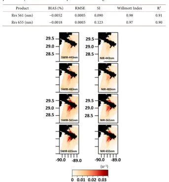
The NIR and SWIR atmospheric correction algorithms showed consistent re-sults at 561 nm (slope = 1.04; R2 _{= 0.91) and 655 nm (slope = 1.02; R}2 _{= 0.90)} (Table 5) in low and moderate turbid water (box 2 and 3). The Rrs (sr−1₎ prod-ucts at 443 nm, 481 nm, 561 nm, and 651 nm from ACOLITE NIR and SWIR atmospheric correction were also compared visually (Figure 5). The left panel presents corrected Rrs products using SWIR approach, and the right panel shows the corrected Rrs product using the NIR approach.

Figure 5 enhances our understanding of the performance of each approach and delivers the knowledge of which approach tends to overestimate and unde-restimate the remote sensing products.

As expected, the NIR correction tended to underestimate Rrs products due to overestimation of the aerosols reflectance. Generally, the highest Rrs values were found in the vicinity of the Mississippi River passes and in shallow coastal waters where significantly influenced by the Mississippi River plume and wave activi-ties. Figure 5 shows that the SWIR approach (right) tended to estimate the higher value of Rrs than NIR approach (left).

3.1.2. Evaluation of Retrieval SPM from Landsat-8 OLI

DOI: 10.4236/ars.2018.72008 113 Advances in Remote Sensing Figure 4. Scatter plots presenting the comparison of Landsat-8 OLI Rrs at (a) 561 nm and (b) 655 nm derived from the Landsat-8 OLI image on 23 April 2016 over the Mississippi River plume using NIR (y-axis) and SWIR (x-axis) atmospheric correction algo-rithms for low and moderate turbid water. The black dashed line is 1:1 and the regression line is drawn in red.

Table 5. Statistics for estimated Landsat-8 OLI Rrs (sr−1_{) products at 561 nm and 655 nm} processed by NIR and SWIR atmospheric correction algorithms in box 2 and 3.

Product BIAS (%) RMSE SI Willmott Index R2

Rrs 561 (nm) −0.0052 0.0005 0.090 0.98 0.91 Rrs 655 (nm) −0.0018 0.0003 0.123 0.97 0.90

DOI: 10.4236/ars.2018.72008 114 Advances in Remote Sensing products corrected by SWIR atmospheric correction algorithm resulted in high-er SPM values compared to the SPM values obtained from Rrs products cor-rected by NIR method.

To validate the SWIR and NIR atmospheric correction approaches and SPM retrieval algorithm using Landsat-8 OLI data, the in situ-measured SPM obtained on 30 July 2014 [50] were compared with Landsat-8 OLI-retrieved SPM concen-tration (Table 6). Only SPM data pairs with a time difference of ±3 hr between in situ and Landsat-8 OLI were used.

The retrieved SPM concentrations using SWIR-corrected Rrs products (at 561 nm and 655 nm) agreed with in situ-measured SPM with an average percentage difference of 10.18%.

Figure 6. Comparison between retrieved SPM concentration (mg.l−1_{) (a) using Landsat-8} OLI SWIR-corrected Rrs (561 nm and 655 nm), and (b) using Landsat-8 OLI NIR-corrected Rrs (561 nm and 655 nm).

Table 6.In situ and OLI-retrieved SPM concentration (mg.l−1_{) using SWIR and NIR}

cor-rected Rrs products on 30 July 2014. The computed percentage difference between in situ and OLI-retrieved SPM using SWIR and NIR atmospheric correction methods.

in situ SPM

(mg∙l−1₎ OLI SPM (mg∙ −1₎

(SWIR method)

OLI SPM (mg∙l−1₎

(NIR method)

Percent Difference Between in situ & OLI

SPM (SWIR method)

Percent Difference Between in situ & OLI

SPM (NIR method)

15.0 14.10 12.62 6.12 17.2

5.0 5.47 5.97 8.97 17.68

16.8 13.62 12.41 20.90 30.05 10.4 11.82 8.86 12.78 15.99

DOI: 10.4236/ars.2018.72008 115 Advances in Remote Sensing Whereas, an average percentage difference of 18.26% was observed be-tween the retrieved SPM concentration using NIR-corrected Rrs products

and in situ-measured SPM. Our results indicated that SWIR atmospheric

cor-rection algorithm was the most appropriated approach to measure SPM concen-trations from Landsat-8 OLI in our study area. The observed discrepancies be-tween Landsat-8 OLI-derived and in situ-measured SPM were likely due to the error associated with field measurements, uncertainties related to the SPM re-trieval algorithms and atmospheric correction algorithms, and the spatial dif-ferences between Landsat-8 OLI pixel location and the sampling locations.

3.2. MODIS Aqua

3.2.1. Comparison of Atmospheric Correction Approaches

The remote sensing reflectance products at 443, 488, 555, and 678 nm from SeaDAS SWIR.NIR algorithm were compared against the SeaDAS MUMM re-sults. Table 7 provides the computed 5th _{and 95}th _{percentile, percentage} differ-ence (Equation (5)), the median ratio (SWIR.NIR to MUMM) and SIQR (Equa-tion (3)) for Rrs products in each type of water.

MUMM SWIR.NIR 100 MUMM SWIR.NIR

2

−

×

+ (5)

Table 7 suggests as the turbidity increased (i.e., influenced by sediment dis-charge from the Mississippi River), the percentage difference increased as well. The MODIS-Aqua SWIR.NIR- and MUMM-corrected remote sensing reflec-tance products were plotted against each other and color-coded based on SPM

Table 7. 5th _{and 95}th _{percentile for MODIS-retrieved Rrs (sr}−1_{) processed by SWIR.NIR and MUMM atmospheric correction} algo-rithms, the percentage difference, median SWIR.NIR to MUMM ratio, and SIQR in box 1, 2 and 3 on 13 September 2013.

Band Box _{SWIR.NIR approach} 5th percentile _{SWIR.NIR approach} 95th percentile _{MUMM approach} 5th percentile _{MUMM approach} 95th percentile Percentage _{Difference Ratio (SIQR)} Median

443 nm

1 0.0008 0.0050 0.0031 0.0060 42.26 0.503 (±0.072) 2 0.0016 0.0023 0.0034 0.0055 38.81 0.443 (±0.024) 3 0.0013 0.0032 0.0027 0.0046 26.16 0.434 (±0.058)

488 nm

1 0.0014 0.0074 0.0042 0.0089 30.02 0.653 (±0.068) 2 0.0025 0.0031 0.0040 0.0057 29.68 0.583 (±0.023) 3 0.0023 0.0035 0.0033 0.0048 27.50 0.568 (±0.036)

555 nm

1 0.0049 0.0128 0.0062 0.0138 30.42 0.837 (±0.034) 2 0.0019 0.0054 0.0049 0.0069 28.38 0.746 (±0.025) 3 0.0015 0.0019 0.0023 0.0029 25.56 0.653 (±0.019)

678 nm

DOI: 10.4236/ars.2018.72008 116 Advances in Remote Sensing concentrations in low to high turbidity waters (Figure 7).

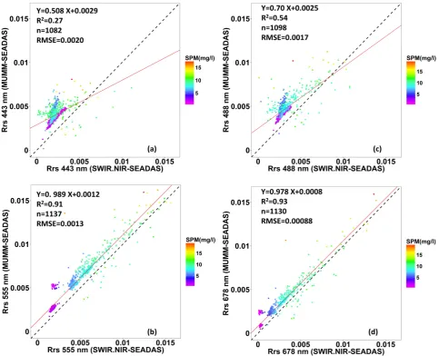
The best agreement was observed between atmospherically corrected Rrs at 678 nm (R2 _{= 0.93, slope = 0.98) followed by Rrs at 555 nm (R}2 _{= 0.91, slope =} 0.99). The low R2 _{was obtained for the shorter wavelengths at 488 nm and 443} nm (0.54 and 0.27). Figures 7(a)-(d) shows that the estimated Rrs resided above 1:1, which implies that the MUMM algorithm tended to estimate the higher val-ue of Rrs than SWIR.NIR. A comparison of atmospheric correction approaches for MODIS-Aqua indicates that SWIR.NIR algorithm estimated the lower value of Rrs than the MUMM algorithm.

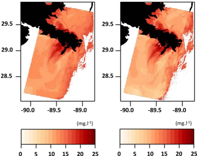
Figure 8 presents the visual comparison of the corrected remote sensing ref-lectance products using SWIR.NIR (left panel) and MUMM (right panel) at-mospheric correction algorithms from SeaDAS in the northern Gulf of Mexico on 13 September 2013. Table 8 presents the statistical parameters for MODIS-Aqua

DOI: 10.4236/ars.2018.72008 117 Advances in Remote Sensing Figure 8. The atmospherically corrected Remote sensing reflectance (Rrs, sr−1_{) at 443 nm,} 488 nm, 555 nm and 678 nm using SWIR.NIR-SeaDAS (right panel), MUMM-SeaDAS (left panel) on 13 September 2013.

Table 8. Statistics for estimated MODIS Rrs (sr−1_{) products processed by SWIR.NIR and} MUMM atmospheric correction algorithms in box 1, 2, 3, and all data points.

Band Box BIAS (%) RMSE SI WI R2

443 nm

1 −0.161 0.0019 0.24 0.43 0.28 2 −0.238 0.0024 0.10 0.26 0.52 3 −0.150 0.0015 0.08 0.42 0.78 All 0.190 0.0020 0.20 0.42 0.27

488 nm

1 −0.190 0.0019 0.07 0.21 0.44 2 −0.160 0.0018 0.17 0.70 0.64 3 −0.120 0.0012 0.06 0.42 0.75 All 0.160 0.0017 0.16 0.58 0.54

555 nm

1 −0.089 0.0009 0.06 0.24 0.30 2 −0.151 0.0016 0.09 0.35 0.48 3 −0.120 0.0014 0.10 0.90 0.87 All 0.110 0.0013 0.41 0.92 0.92

678 nm

DOI: 10.4236/ars.2018.72008 118 Advances in Remote Sensing Rrs products corrected using SWIR.NIR and MUMM atmospheric correction algorithm. The results indicate that the agreement between the Rrs products processed by SWIR.NIR and MUMM decreased as the turbidity increased. For example, at 678 nm the R2 _{value decreased from 0.87 (in box 3; low turbid) to} 0.38 (in box 1; high turbid) as the distance from the Mississippi River which supplies sediment decreased.

Figure 9 presents the MODIS-derived SPM concentration maps using cor-rected Rrs (555 nm and 678 nm) by SWIR.NIR (Figure 6(a)) and MUMM (Figure 6(b)) approaches on 13 September 2013. In general, SPM concentration values from corrected Rrs by MUMM approach were higher than SPM concen-tration values retrieved from SWIR.NIR-corrected Rrs. Converse to the cor-rected Landsat-8 OLI Rrs products, the point cloud feature dipping below 1:1 (Figure 3) was not observed in Figure 7. The lower radiometric sensitivity of MODIS may explain why this feature was not observed for MODIS-Aqua. The MODIS data from September 2013 were collected when the Mississippi River exhibited a much lower discharge (~6698.4 m3_∙s−1 _{at Belle Chasse station)} compared to the discharge of the Mississippi River at Belle Chasse during the Landsat-8 OLI overpass (~22,115 m3_∙s−1_{) in April 2016, which could lead to} sub-stantially more turbid waters, and thus brighter red reflectance. The maximum value of ~0.0155 sr−1 _{was observed in high turbidity at Rrs (655 nm) retrieved} from MODIS (Figure 7(b)), whereas the maximum value of Landsat-8 OLI Rrs at 655 nm on 23 April 2016 was 0.035 sr−1 _{(Figure 3(g)). In addition, the use} of high-quality SWIR bands of Landsat-8 OLI leads to an accurate quantification

DOI: 10.4236/ars.2018.72008 119 Advances in Remote Sensing of the aerosol contribution to the top of the atmosphere and Rrs products. Whe-reas, MODIS SWIR bands (1240 nm and 2130 nm) are quite noisy due to the low SNR, which is considered as a shortcoming of the sensor in terms of atmos-pheric correction approach [57].

3.2.2. Evaluation of Retrieved SPM from MODIS-Aqua

Figure 10 shows the match-ups between MODIS-derived SPM concentration and in situ-measured SPM concentration. We observed a relatively high agree-ment (Figure 10(a)) between MODIS-derived SPM concentration processed with SWIR.NIR atmosphere correction algorithm (R2 _{= 0.79, bias = 0.63), while} retrieved SPM concentration processed with MUMM algorithm suggested a lower agreement (Figure 10(b)) with field data (R2 _{= 0.76, bias = 1.23), see} Ta-ble 1 and Figure 2 for data points used in the comparison. Note that to perfume the match-up comparison, the time difference of ±3 hr between in situ-measured SPM and MODIS-Aqua overpasses was considered.

The performance of each atmospheric correction algorithms in retrieving SPM was assessed using BIAS, RMSE, SI, and R2 _{(Table 9). The comparison} be-tween in situ SPM and MODIS-derived SPM suggested that the SWIR.NIR at-mosphere correction algorithm was the most appropriate algorithm in our study area (Figure 10 and Table 9). The observed disagreement between MODIS-derived and in situ-measured SPM was attributable to the low spatial resolution (1 km) of MODIS, low SNR values of MODIS-Aqua SWIR bands. In addition, errors

Figure 10. Comparison of in situ-measured SPM concentration (mg.l−1_{) with MODIS Aqua-retrieved SPM concentration} processed using (a) SWIR.NIR and (b) MUMM.

Table 9. Statistics for SPM concentration obtained from MODIS-Aqua Rrs products cor-rected by SWIR.NIR and MUMM atmospheric correction methods.

Product BIAS RMSE SI R2

DOI: 10.4236/ars.2018.72008 120 Advances in Remote Sensing associated with the atmospheric correction processes and SPM retrieval algo-rithm would exacerbate the disagreement between satellite-derived and field SPM concentration.

4. Summary and Conclusions

To monitor SPM dynamics using satellite data in Louisiana coastal and shelf wa-ters, appropriate atmospheric correction algorithms and robust SPM retrieval al-gorithms are required. The performance of the four atmospheric correction algo-rithms was evaluated: the SWIR and NIR atmospheric correction algoalgo-rithms for Landsat-8 OLI and the MUMM along with the SWIR.NIR atmospheric correction algorithm for MODIS-Aqua. The results suggested that the NIR algorithm re-trieved lower values of Rrs products from Landsat-8 OLI in high turbidity waters. The SPM retrieval algorithm was applied to the corrected Rrs products from Landsat-8 OLI and MODIS-Aqua to estimate SPM concentrations. The Land-sat-8 OLI Rrs products corrected atmospherically by the SWIR algorithm, re-trieved more accurate SPM concentrations in our study area. In addition, a good agreement was found between MODIS-derived SPM processed with SWIR.NIR algorithm and field data. However, more in situ SPM data are needed to stress the robustness of these algorithms in our study area. In addition, it is strongly suggested to evaluate the performance of the revised Rrs (NIR) model [58] in the northern Gulf of Mexico. This model has been implemented by the NASA Ocean Biology Processing Group (OBPG) in the operational processing of satel-lite ocean color sensor data.

The observed imperfections between satellite-derived and in situ-measured SPM concentrations could be due to several factors related to the satellite’s cha-racteristics and errors and assumptions in the SPM retrieval algorithm used in this study [59]. The results underline the necessity of in situ measurements of Rrs products and SPM data to validate SPM retrieval algorithms. Furthermore, our findings highlight that multi-conditional SPM retrieval algorithms based on turbidity level must be considered in our study region. The use of mul-ti-conditional SPM retrieval algorithms switching from red-NIR algorithms to visible band ratio algorithms would improve the accuracy of retrieved SPM. Hence, hyperspectral reflectance measurements must be carried out over low- to high turbidity waters.

SPM concentrations maps derived from satellites can be used to validate se-diment transport and ecological models. The results of the present study are be-ing used in an ongobe-ing study for the numerical simulation of sediment transport in Gulf of Mexico, over the Louisiana shelf.

References

DOI: 10.4236/ars.2018.72008 121 Advances in Remote Sensing https://doi.org/10.1016/j.rse.2017.01.039

[2] Ma, G., Han, Y., Niroomandi, A., Lou, S. and Liu, S. (2015) Numerical Study of Se-diment Transport on a Tidal Flat with a Patch of Vegetation. Ocean Dynamics, 65, 203-222.https://doi.org/10.1007/s10236-014-0804-8

[3] Niroomandi, A., Ma, G., Su, S.-F., Gu, F. and Qi, D. (2017) Sediment Flux and Se-diment-Induced Stratification in the Changjiang Estuary. Journal of Marine Science and Technology, 1-15.

[4] Kirk, J.T. (1994) Light and Photosynthesis in Aquatic Ecosystems. 3rd Edition, Cambridge University Press, Cambridge.

[5] Allahdadi, M.N, Felix, J., Stone, W.G. and D’Sa., E.J. (2011) The Fate of Sediment Plumes Discharged from the Mississippi and Atchafalaya Rivers: An Integrated Ob-servation and Modeling Study for the Louisiana Shelf, USA. Proceedings of the Coastal Sediments, Miami, 2-6 May 2011, 2212-2225.

https://doi.org/10.1142/9789814355537_0166

[6] Blaas, M., El Serafy, G.Y.H., van Kessel, T., de Boer, G.J., Eleveld, M.A. and Van der Woerd, H.J. (2007) Data Model Integration of SPM Transport in the Dutch Coastal Zone. Proceedings of the Joint 2007 EUMETSAT/AMS Conference, Darmstadt. [7] D’Sa, E.J., Roberts, H. and Allahdadi, M.N. (2011) Suspended Particulate Matter

Dynamics along the Louisiana-Texas Coast from Satellite Observations. Proceed-ings of the Coastal Sediments, Miami, 2-6 May 2011, 2390-2402.

https://doi.org/10.1142/9789814355537_0179

[8] Miller, R.L. and McKee, B.A. (2004) Using MODIS Terra 250 m Imagery to Map Concentrations of Total Suspended Matter in Coastal Waters. Remote Sensing of Environment, 93, 259-266. https://doi.org/10.1016/j.rse.2004.07.012

[9] Vanhellemont, Q. and Ruddick, K. (2014) Turbid Wakes Associated with Offshore Wind Turbines Observed with Landsat 8. Remote Sensing of Environment, 145, 105-115. https://doi.org/10.1016/j.rse.2014.01.009

[10] Ody, A., Doxaran, D., Vanhellemont, Q., Nechad, B., Novoa, S., Many, G., et al. (2016) Potential of High Spatial and Temporal Ocean Color Satellite Data to Study the Dynamics of Suspended Particles in a Micro-Tidal River Plume. Remote Sens-ing, 8, 245. https://doi.org/10.3390/rs8030245

[11] Novoa, S., Doxaran, D., Ody, A., Vanhellemont, Q., Lafon, V., Lubac, B., et al. (2017) Atmospheric Corrections and Multi-Conditional Algorithm for Mul-ti-Sensor Remote Sensing of Suspended Particulate Matter in Low-to-High Turbid-ity Levels Coastal Waters. Remote Sensing, 9, 61. https://doi.org/10.3390/rs9010061 [12] Vanhellemont, Q. and Ruddick, K. (2015) Advantages of High Quality SWIR Bands

for Ocean Colour Processing: Examples from Landsat-8. Remote Sensing of Envi-ronment, 161, 89-106. https://doi.org/10.1016/j.rse.2015.02.007

[13] Hestir, E.L., Brando, V.E., Bresciani, M., Giardino, C., Matta, E., Villa, P., et al. (2015) Measuring Freshwater Aquatic Ecosystems: The Need for a Hyperspectral Global Mapping Satellite Mission. Remote Sensing of Environment, 167, 181-195. https://doi.org/10.1016/j.rse.2015.05.023

[14] Allahdadi, M.N., Jose, F., D’Sa, E.J. and Ko, D.S. (2017) Effect of Wind, River Dis-charge, and Outer-Shelf Phenomena on Circulation Dynamics of the Atchafalaya Bay and Shelf. Ocean Engineering, 129, 567-580.

https://doi.org/10.1016/j.oceaneng.2016.10.035

[15] Allahdadi, M.N. and Li, C. (2017) Numerical Simulation of Louisiana Shelf Circula-tion under Hurricane Katrina. Journal of Coastal Research, 34, 67-80.

DOI: 10.4236/ars.2018.72008 122 Advances in Remote Sensing MSc Theses, Louisiana State University, Baton Rouge.

[17] Georgiou, I.Y., FitzGerald, D.M. and Stone, G.W. (2005) The Impact of Physical Processes along the Louisiana Coast. Journal of Coastal Research, 44, 72-89. [18] Roberts, H.H., Huh, O.K., Hsu, S.A., Rouse, L.J. and Rickman, D. (1987) Impact of

Coldfront Passages on Geomorphic Evolution and Sediment Dynamics of the Com-plex Louisiana Coast. Proceedings of a Specialty Conference, New Orleans.

[19] Li, C., Roberts, H., Stone, G.W., Weeks, E. and Luo, Y. (2011) Wind Surge and Saltwater Intrusion in Atchafalaya Bay during Onshore Winds Prior to Cold Front Passage. Hydrobiologia, 658, 27-39. https://doi.org/10.1007/s10750-010-0467-5 [20] Walker, N.D. and Hammack, A.B. (2000) Impacts of Winter Storms on Circulation

and Sediment Transport: Atchafalaya-Vermilion Bay Region, Louisiana, U.S.A. Journal of Coastal Research, 16, 996-1010.

[21] Chen, J., D’Sa, E., Cui, T. and Zhang, X. (2013) A Semi-Analytical Total Suspended Sediment Retrieval Model in Turbid Coastal Waters: A Case Study in Changjiang River Estuary. Optics Express, 21, 13018-13031.

https://doi.org/10.1364/OE.21.013018

[22] Dogliotti, A.I., Ruddick, K.G., Nechad, B., Doxaran, D. and Knaeps, E. (2015) A Single Algorithm to Retrieve Turbidity from Remotely-Sensed Data in All Coastal and Estuarine Waters. Remote Sensing of Environment, 156, 157-168.

https://doi.org/10.1016/j.rse.2014.09.020

[23] D’Sa, E.J., Miller, R.L. and McKee, B.A. (2007) Suspended Particulate Matter Dy-namics in Coastal Waters from Ocean Color: Application to the Northern Gulf of Mexico. Geophysical Research Letters, 34, L23611.

[24] Nechad, B., Ruddick, K.G. and Park, Y. (2010) Calibration and Validation of a Ge-neric Multisensor Algorithm for Mapping of Total Suspended Matter in Turbid Waters. Remote Sensing of Environment, 114, 854-866.

https://doi.org/10.1016/j.rse.2009.11.022

[25] Nechad, B., Alvera-Azcaràte, A., Ruddick, K. and Greenwood, N. (2011) Recon-struction of MODIS Total Suspended Matter Time Series Maps by DINEOF and Validation with Autonomous Platform Data. Ocean Dynamics, 61, 1205-1214. https://doi.org/10.1007/s10236-011-0425-4

[26] Van der Woerd, H. and Pasterkamp, R. (2004) Mapping of the North Sea Turbid Coastal Waters Using SeaWiFS Data. Canadian Journal of Remote Sensing, 30, 44-53.https://doi.org/10.5589/m03-051

[27] Doxaran, D., Froidefond, J.-M., Lavender, S. and Castaing, P. (2002) Spectral Sig-nature of Highly Turbid Waters: Application with SPOT Data to Quantify Sus-pended Particulate Matter Concentrations. Remote Sensing of Environment, 81, 149-161.https://doi.org/10.1016/S0034-4257(01)00341-8

[28] Shen, F., Verhoef, W., Zhou, Y., Salama, M.S. and Liu, X. (2010) Satellite Estimates of Wide-Range Suspended Sediment Concentrations in Changjiang (Yangtze) Est-uary Using MERIS Data. Estuaries and Coasts, 33, 1420-1429.

https://doi.org/10.1007/s12237-010-9313-2

[29] Doxaran, D., Froidefond, J.-M., Castaing, P. and Babin, M. (2009) Dynamics of the Turbidity Maximum Zone in a Macrotidal Estuary (the Gironde, France): Observa-tions from Field and MODIS Satellite Data. Estuarine, Coastal and Shelf Science, 81, 321-332. https://doi.org/10.1016/j.ecss.2008.11.013

DOI: 10.4236/ars.2018.72008 123 Advances in Remote Sensing [31] Gordon, H.R. and Wang, M. (1994) Retrieval of Water-Leaving Radiance and

Aerosol Optical Thickness over the Oceans with SeaWiFS: A Preliminary Algo-rithm. Applied Optics, 33, 443-452.https://doi.org/10.1364/AO.33.000443

[32] Ruddick, K.G., Ovidio, F. and Rijkeboer, M. (2000) Atmospheric Correction of SeaWiFS Imagery for Turbid Coastal and Inland Waters. Applied Optics, 39, 897-912.https://doi.org/10.1364/AO.39.000897

[33] Dogliotti, A., Ruddick, K., Nechad, B. and Lasta, C. (2011) Improving Water Ref-lectance Retrieval from MODIS Imagery in the Highly Turbid Waters of La Plata River. Proceedings of the 6th International Conference Current Problems in Optics of Natural Waters, St. Petersburg, 6-9 September 2011, 1-8.

[34] Wang, M. and Shi, W. (2007) The NIR-SWIR Combined Atmospheric Correction Approach for MODIS Ocean Color Data Processing. Optics Express, 15, 15722- 15733.https://doi.org/10.1364/OE.15.015722

[35] Vanhellemont, Q., Neukermans, G. and Ruddick, K. (2014) Synergy between Po-lar-Orbiting and Geostationary Sensors: Remote Sensing of the Ocean at High Spa-tial and High Temporal Resolution. Remote Sensing of Environment, 146, 49-62. https://doi.org/10.1016/j.rse.2013.03.035

[36] Wang, M. (2007) Remote Sensing of the Ocean Contributions from Ultraviolet to Near-Infrared Using the Shortwave Infrared Bands: Simulations. Applied Optics, 46, 1535-1547.https://doi.org/10.1364/AO.46.001535

[37] Wang, M., Son, S. and Shi, W. (2009) Evaluation of MODIS SWIR and NIR-SWIR Atmospheric Correction Algorithms Using SeaBASS Data. Remote Sensing of En-vironment, 113, 635-644.https://doi.org/10.1016/j.rse.2008.11.005

[38] Milliman, J.D. and Farnsworth, K.L. (2012) River Discharge to the Coastal Ocean: A Global Synthesis. Cambridge University Press, Cambridge.

[39] Twilley, R.R., Bentley, S.J., Chen, Q., Edmonds, D.A., Hagen, S.C., Lam, N.S.-N., et al. (2016) Co-Evolution of Wetland Landscapes, Flooding, and Human Settlement in the Mississippi River Delta Plain. Sustainability Science, 11, 711-731.

https://doi.org/10.1007/s11625-016-0374-4

[40] Hu, C., Nelson, J.R., Johns, E., Chen, Z., Weisberg, R.H. and Müller-Karger, F.E. (2005) Mississippi River Water in the Florida Straits and in the Gulf Stream off Georgia in Summer 2004. Geophysical Research Letters, 32, L14606.

https://doi.org/10.1029/2005GL022942

[41] Meade, R.H. and Parker, R.S. (1984) Sediment in Rivers of the United States Na-tional Water Summary, 1984 Water Supply Paper. US Geological Survey 1985, Res-ton VA, 40-60.

[42] Dinnel, S.P. and Wiseman, W.J. (1986) Fresh Water on the Louisiana and Texas Shelf. Continental Shelf Research, 6, 765-784.

https://doi.org/10.1016/0278-4343(86)90036-1

[43] Lohrenz, S.E., Fahnenstiel, G.L., Redalje, D.G., Lang, G.A., Dagg, M.J., Whitledge, T.E., et al. (1999) Nutrients, Irradiance, and Mixing as Factors Regulating Primary Production in Coastal Waters Impacted by the Mississippi River Plume. Continen-tal Shelf Research, 19, 1113-1141.https://doi.org/10.1016/S0278-4343(99)00012-6 [44] Rabalais, N.N., Turner, R.E., JustiĆ, D., Dortch, Q., Wiseman, W.J. and Gupta, B.K.S.

(1996) Nutrient Changes in the Mississippi River and System Responses on the Ad-jacent Continental Shelf. Estuaries, 19, 386-407.https://doi.org/10.2307/1352458 [45] Tehrani, N.C., D’Sa, E.J., Osburn, C.L., Bianchi, T.S. and Schaeffer, B.A. (2013)

DOI: 10.4236/ars.2018.72008 124 Advances in Remote Sensing Spectroradiometer (MODIS) and MERIS Sensors: Case Study for the Northern Gulf of Mexico. Remote Sensing, 5, 1439-1464. https://doi.org/10.3390/rs5031439 [46] Cochrane, J.D. and Kelly, F.J. (1986) Low-Frequency Circulation on the Texas-

Louisiana Continental Shelf. Journal of Geophysical Research: Oceans, 91, 10645- 10659. https://doi.org/10.1029/JC091iC09p10645

[47] Chaichitehrani, N., D’Sa, E.J., Ko, D.S., Walker, N.D., Osburn, C.L. and Chen, R.F. (2013) Colored Dissolved Organic Matter Dynamics in the Northern Gulf of Mex-ico from Ocean Color and Numerical Model Results. Journal of Coastal Research, 30, 800-814.

[48] Hitchcock, G.L., Wiseman, W.J., Boicourt, W.C., Mariano, A.J., Walker, N., Nelsen, T.A., et al. (1997) Property Fields in an Effluent Plume of the Mississippi River. Journal of Marine Systems, 12, 109-126.

https://doi.org/10.1016/S0924-7963(96)00092-9

[49] Salisbury, J.E., Campbell, J.W., Linder, E., David Meeker, L., Müller-Karger, F.E. and Vörösmarty, C.J. (2004) On the Seasonal Correlation of Surface Particle Fields with Wind Stress and Mississippi Discharge in the Northern Gulf of Mexico. Deep Sea Research Part II: Topical Studies in Oceanography, 51, 1187-1203.

https://doi.org/10.1016/S0967-0645(04)00107-9

[50] Rabalais, N.N. (2014) Physical (Hydrography), Chemical (CTD), and Biological (Water Quality) Processes of the Texas-Louisiana Continental Shelf (NCEI Acces-sion 0161219) VerAcces-sion 1.1. NOAA National Centers for Environmental Informa-tion. https://ftp.nodc.noaa.gov/nodc/archive/arc0106/0161219/

[51] Pahlevan, N., Lee, Z., Wei, J., Schaaf, C.B., Schott, J.R. and Berk, A. (2014) On-Orbit Radiometric Characterization of OLI (Landsat-8) for Applications in Aquatic Re-mote Sensing. Remote Sensing of Environment, 154, 272-284.

https://doi.org/10.1016/j.rse.2014.08.001

[52] Bailey, S.W. and Werdell, P.J. (2006) A Multi-Sensor Approach for the On-Orbit Validation of Ocean Color Satellite Data Products. Remote Sensing of Environment, 102, 12-23.https://doi.org/10.1016/j.rse.2006.01.015

[53] Lee, Z., Mannino, A., Muller-Karger, F.E., Ondrusek, M. and Salisbury, J. (2013) GEO-CAPE, GOMEX 2013. SeaWiFS Bio-Optical Archive and Storage System (SeaBASS). NASA. https://seabass.gsfc.nasa.gov/cruise/gomex_2013

[54] Rabalais, N.N. (2012) Physical (Hydrography), Chemical (CTD), and Biological (Water Quality) Processes of the Texas-Louisiana Continental Shelf (NCEI Acces-sion 0162101) VerAcces-sion 1.1. NOAA National Centers for Environmental Informa-tion. http://ftp.nodc.noaa.gov/nodc/archive/arc0106/0162101/

[55] Rabalais, N.N. (2013) Physical (Hydrography), Chemical (CTD), and Biological (Water Quality) Processes of the Texas-Louisiana Continental Shelf, 2013 (NCEI Accession 0162440) Version 1.1. NOAA National Centers for Environmental In-formation. http://ftp.nodc.noaa.gov/nodc/archive/arc0107/0162440/

[56] Willmott, C.J. (1981) On the Validation of Models. Physical Geography, 2, 184-194. [57] Wang, M. and Shi, W. (2012) Sensor Noise Effects of the SWIR Bands on MODIS-

Derived Ocean Color Products. IEEE Transactions on Geoscience and Remote Sensing, 50, 3280-3292. https://doi.org/10.1109/TGRS.2012.2183376

[58] Bailey, S.W., Franz, B.A. and Werdell, P.J. (2010) Estimation of Near-Infrared Wa-ter-Leaving Reflectance for Satellite Ocean Color Data Processing. Optics Express, 18, 7521-7527. https://doi.org/10.1364/OE.18.007521