Language Modeling for Code Mixing: The Role of Linguistic Theory based Synthetic Data

1543

Language Modeling for Code-Mixing:

The Role of Linguistic Theory based Synthetic Data

Adithya Pratapa1 Gayatri Bhat2∗ Monojit Choudhury1 Sunayana Sitaram1 Sandipan Dandapat3 _{Kalika Bali}1

1_{Microsoft Research, Bangalore, India}

2_{Language Technology Institute, Carnegie Mellon University} 3_{Microsoft R&D, Hyderabad, India}

1_{{t-pradi, monojitc, sunayana.sitaram, kalikab}@microsoft.com,} 2_{[email protected],}3_{[email protected]}

Abstract

Training language models for Code-mixed (CM) language is known to be a diffi-cult problem because of lack of data com-pounded by the increased confusability due to the presence of more than one lan-guage. We present a computational tech-nique for creation of grammatically valid artificial CM data based on the Equiva-lence Constraint Theory. We show that when training examples are sampled ap-propriately from this synthetic data and presented in certain order (aka training curriculum) along with monolingual and real CM data, it can significantly reduce the perplexity of an RNN-based language model. We also show that randomly gener-ated CM data does not help in decreasing the perplexity of the LMs.

1 Introduction

Code-switchingorcode-mixing(CM) refers to the juxtaposition of linguistic units from two or more languages in a single conversation or sometimes even a single utterance.1 It is quite commonly ob-served in speech conversations of multilingual so-cieties across the world. Although, traditionally, CM has been associated with informal or casual speech, there is evidence that in several societies, such as urban India and Mexico, CM has become the default code of communication (Parshad et al., 2016), and it has also pervaded written text, espe-cially in computer-mediated communication and social media (Rijhwani et al.,2017).

∗

Work done during author’s internship at Microsoft Re-search

1_{According to some linguists, code-switching refers to}

inter-sentential mixing of languages, whereas code-mixing refers to intra-sentential mixing. Since the latter is more gen-eral, we will use code-mixing in this paper to mean both.

It is, therefore, imperative to build NLP tech-nology for CM text and speech. There have been some efforts towards building of Automatic Speech Recognition Systems and TTS for CM speech (Li and Fung,2013,2014;Gebhardt,2011; Sitaram et al., 2016), and tasks like language identification (Solorio et al., 2014;Barman et al., 2014), POS tagging (Vyas et al., 2014; Solorio and Liu, 2008), parsing and sentiment analy-sis (Sharma et al.,2016;Prabhu et al.,2016;Rudra et al.,2016) for CM text. Nevertheless, the accura-cies of all these systems are much lower than their monolingual counterparts, primarily due to lack of enough data.

Intuitively, since CM happens between two (or more languages), one would typically need twice as much, if not more, data to train a CM sys-tem. Furthermore, any CM corpus will contain large chunks of monolingual fragments, and rel-atively far fewer code-switching points, which are extremely important to learn patterns of CM from data. This implies that the amount of data required would not just be twice, but probably 10 or 100 times more than that for training a monolingual system with similar accuracy. On the other hand, apart from user-generated content on the Web and social media, it is extremely difficult to gather large volumes of CM data because (a) CM is rare in formal text, and (b) speech data is hard to gather and even harder to transcribe.

amount of real CM data to train a CMLanguage Model (LM). Our experiments show that, when trained following certain sampling strategies and training curriculum, the synthetic CM sentences are indeed able to improve the perplexity of the trained LM over a baseline model that uses only monolingual and real CM data.

LM is useful for a variety of downstream NLP tasks such as Speech Recognition and Machine Translation. By definition, it is a discriminator be-tween natural and unnatural language data. The fact that linguistically constrained synthetic data can be used to develop better LM for CM text is, on one hand an indirect statistical and task-based validation of the linguistic theory used to generate the data, and on the other hand an indication that the approach in general is promising and can help solve the issue of data scarcity for a variety of NLP tasks for CM text and speech.

2 Generating Synthetic Code-mixed Data

There is a large and growing body of linguis-tic research regarding the occurrence, syntac-tic structure and pragmasyntac-tic functions of code-mixing in multilingual communities across the world. This includes many attempts to explain the grammatical constraints on CM, with three of the most widely-accepted being the Embedded-Matrix(Joshi,1985;Myers-Scotton,1993,1995), theEquivalence Constraint(EC) (Poplack,1980; Sankoff, 1998) and the Functional Head Con-straint(DiSciullo et al.,1986;Belazi et al.,1994) theories.

For our experiments, we generate CM sentences as per the EC theory, since it explains a range of interesting CM patterns beyond lexical substitu-tion and is also suitable for computasubstitu-tional model-ing. Further, in a brief human-evaluation we con-ducted, we found that it is representative of real CM usage. In this section, we list the assumptions made by the EC theory, briefly explain the theory, and then describe how we generate CM sentences as per this theory.

2.1 Assumptions of the EC Theory

Consider two languages L1 and L2 that are be-ing mixed. The EC Theory assumes that both languages are defined by context-free grammars G1 and G2. It also assumes that every non-terminal category X1 in G1 has a corresponding non-terminal category X2in G2and that every

ter-minal symbol (or word) w1 in G1 has a corre-sponding terminal symbol w2 in G2. Finally, it assumes that every production rule in L1has a cor-respondingrule in L2 - i.e, the non-terminal cate-gories on the left-hand side of the two rules cor-respond to each other, and every category/symbol on the right-hand side of one rule corresponds to a category/symbol on the right-hand side of the other rule.

All these correspondences must also hold vice-versa (between languages L2 and L1), which im-plies that the two grammars can only differ in the ordering of categories/symbols on the right-hand side of any production rule. As a result, any sen-tence in L1has a corresponding translation in L2, with their parse trees being equivalent except for the ordering of sibling nodes. Fig.1(a) and (b) illustrate one such sentence pair in English and Spanish and their parse-trees. The EC Theory de-scribes a CM sentence as a constrained combina-tion of two such equivalent sentences.

While the assumptions listed above are quite strong, they do not prevent the EC Theory from being applied to two natural languages whose grammars do not correspond as described above. We apply a simple but effective strategy to recon-cile the structures of a sentence and its translation - if any corresponding subtrees of the two parse trees do not have equivalent structures, we col-lapse each of these subtrees to a single node. Ac-counting for the actual asymmetry between a pair of languages will certainly allow for the genera-tion of more CM variants of any L1-L2 sentence pair. However, in our experiments, this strategy retains most of the structural information in the parse trees, and allows for the generation of up to thousands of CM variants of a single sentence pair.

2.2 The Equivalence Constraint Theory

(a) SE VPE PPE NPE NNE house JJE white DTE a INE in VBZE lives NPE PRPE She

(b) SS

VPS PPS NPS JJS blanca NNS casa DTS una INS en VBZS vive NPS PRPS Elle (c) S VP PP NP JJ* white NNS casa DTS una INS en VBZE lives NPS PRPS Elle (d) S VP PP NPS JJS blanca NNS casa DTS una INE in VBZE lives NPS PRPS Elle

Figure 1: Parse trees of a pair of equivalent (a) English and (b) Spanish sentences, with corresponding hierarchical structure (due to production rules), internal nodes (non-terminal categories) and leaf nodes (terminal symbols), and parse trees of (c) incorrectly code-mixed and (d) correctly code-mixed variants of these sentences (as per the EC theory).

constituent. (Sankoff,1998) This guarantees that the parse tree of a sentence so produced will have the same hierarchical structure as the two mono-lingual parse trees (Fig.1(c) and (d)).

The EC theory also requires that any mono-lingual fragment that occurs in the CM sentence must occur in one of the monolingual sentences (in the running example, the fragmentuna blanca would be disallowed since it does not appear in the Spanish sentence).

Switch-point identification. To ensure that the CM sentence does not at any point deviate from both monolingual grammars, the EC theory im-poses certain constraints on its parse tree. To this end and in order to identify the code-switching points in a generated sentence, nodes in its parse tree are assigned language labels according to the following rules: All leaf nodes are labeled by the languages of their symbols. If all the children of any internal node share a common label, the inter-nal node is also labeled with that language. Any node that is out of rank-order among its siblings according to one language is labeled with the other language. (See labeling in Fig.1(c) and (d)) If any node acquires labels of both languages during this process (such as the node marked with an asterisk in Fig.1(c)), the sentence is disallowed as per the EC theory. In the labeled tree, any pair of adjacent sibling nodes with contrasting labels are said to be at aswitch-point(SP).

Equivalence constraint. Every switch-point identified in the generated sentence must abide by the EC. LetU → U1U2...UnandV →V1V2...Vn

be corresponding rules applied in the two mono-lingual parse trees, and nodesUi andVi+1 be ad-jacent in the CM parse tree. This pair of nodes is a switch-point, and it only abides by the EC if every node in U1...Ui has a corresponding node

in V1...Vi. This is true for the switch-point in

Fig.1(d), and indicates that the two grammars are ‘equivalent’ at the code-switch point. More im-portantly, it shows that switching languages at this point does not require another switch later in the sentence. If every switch-point in the generated sentence abides by the EC, the generated sentence is allowed by the EC theory.

2.3 System Description

We assume that the input to the generation model is a pair of parallel sentences in L1 and L2, along with word level alignments. For our experiments, L1 and L2 are English and Spanish, and Sec 3.2 describes how we create the input set. We use the Stanford Parser (Klein and Manning,2003) to parse the English sentence.

Projecting parses. We use the alignments to project the English parse tree onto the Spanish sentence in two steps: (1) We first replace every word in the English parse tree with its Spanish equivalent (2) We re-order the child nodes of each internal node in the tree such that their left-to-right order is as in the Spanish sentence. For instance, after replacing every English word in Fig.1(a) with its corresponding Spanish word, we interchange the positions ofcasaandblancato arrive Fig.1(b). For a pair of parallel sentences that follow all the assumptions of the EC theory, these steps can be performed without exception and result in the cre-ation of a Spanish parse tree with the same hierar-chical structure as the English parse.

(a) SE

VPE

VPE

NPE

PRPE

it VBE

do MDE

will NPE

NNPE

She

(b) SE

VPE

NPE

PRPE

it MD+VBE

do will NPE

NNPE

She

(c) SS

VPS

MD+VBS

har´a NPS

PRPS

lo NPS

NNPS

<>

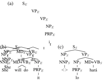
Figure 2: (a) The parse of an English sentence as per Stanford CoreNLP. This parse is projected onto the parallel Spanish sentence Lo har´a and modified during this process, to produce corre-sponding (b) English and (c) Spanish parse trees.

same word(s) in the other language are collapsed into a single multi-word node, and the entire sub-tree between these collapsed nodes and their clos-est common ancclos-estor is flattened to accommo-date this change (example in Fig.2). While these changes do result in slightly unnatural or simpli-fied parse trees, they are used very sparingly since English and Spanish have very compatible gram-mars.

Generating CS sentences. The number of CS sentences that can be produced by combining a corresponding pair of English and Spanish sen-tences increases exponentially with the length of the sentences. Instead of generating these sen-tences exhaustively, we use the parses to construct a finite-state automaton that succinctly captures the acceptable CS sentences. Since the CS sen-tence must have the same hierarchical structure as the monolingual sentences, we construct the au-tomaton during a post-order traversal of the mono-lingual parses. An automaton is constructed at each node by (1) concatenating the automatons constructed at its child nodes, (2) splitting states and removing transitions to ensure that the EC the-ory is not violated. The last automaton to be con-structed, which is associated with the root node, accepts all the CS sentences that can be generated using the monolingual parses. We do not provide the exact details of automaton construction here, but we plan to release our code in the near future.

3 Datasets

In this work, we use three types of language data: monolingual data in English and Spanish (Mono), real code-mixed data (rCM), and artificial or gen-erated code-mixed data (gCM). In this section, we describe these datasets and their CM properties. We begin with description of some metrics that we shall use for quantification of the complexity of a CM dataset.

3.1 Measuring CM Complexity

The CM data, both real and artificial, can vary in the their relative usage and ordering of L1 and L2 words, and thereby, significantly affect down-stream applications like language modeling. We use the following metrics to estimate the amount and complexity of code-mixing in the datasets.

Switch-point (SP): As defined in the last sec-tion, switch-points are points within a sentence where the languages of the words on the two sides are different. Intuitively, sentences that have more number of SPs are inherently more complex. We also define the metric SP Fraction (SPF) as the number of SP in a sentence divided by the total number of word boundaries in the sentence.

Code mixing index (CMI):Proposed by Gam-back and Das (2014, 2016), CMI quantifies the amount of code mixing in a corpus by accounting for the language distribution as well as the switch-ing between them. LetN be the number of lan-guage tokens,xan utterance; lettLi be the tokens

in languageLi,P be the number of code

switch-ing points in x. Then, the Code mixed index per utterance,Cu(x)forxcomputed as follows,

Cu(x) =

(N(x)−maxLi∈L{tLi}(x)) +P(x)

N(x) (1)

Note that all the metrics can be computed at the sentence level as well as at the corpus level by av-eraging the values for all the sentences in a corpus.

3.2 Real Datasets

Dataset # Tweets # Words CMI SPF Mono

English 100K 850K (48K) 0 0

Spanish 100K 860K (61K) 0 0

rCM

Train 100K 1.4M (91K) 0.31 0.105

Validation 100K 1.4M (91K) 0.31 0.106 Test-17 83K 1.1M (82K) 0.31 0.104 Test-14 13K 138K (16K) 0.12 0.06

gCM 31M 463M (79K) 0.75 0.35

Table 1: Size of the datasets. Numbers in paren-thesis show the vocabulary size, i.e., the no. of unique words.

For our experiments, we use a subset of the tweets collected by Rijhwani et al. (2017) that were automatically identified as English, Span-ish or EnglSpan-ish-SpanSpan-ish CM. The authors provided us around 4.5M monolingual tweets per language, and 283K CM tweets. These were already dedu-plicated and tagged for hashtags, URLs, emoti-cons and language labels automatically through the method proposed in the paper. Table1shows the sizes of the various datasets, which are also de-scribed below.

Mono: 50K tweets were sampled for Spanish and English from the entire collection of monolin-gual tweets. The Spanish tweets were translated to English and vice versa, which gives us a total of 100K monolingual tweets in each language. We shall refer to this dataset asMono. The sampling strategy and reason for generating translations will become apparent in Sec.3.3.

rCM: We use two real CM datasets in our ex-periment. The 283K real CM tweets provided by Rijhwani et al.(2017) were randomly divided into training, validation and test sets of nearly equal sizes. Note that for most of our experiments, we will use a very small subset of the training set con-sisting of 5000 tweets as train data, because the fundamental assumption of this work is that very little amount of CM data is available for most lan-guage pairs (which is in fact true for most pairs beyond some very popularly mixed languages like English-Spanish). Nevertheless, the much larger training set is required for studying the effect of varying the amount of real CM data on our mod-els. We shall refer to this training dataset as rCM. The test set with 83K tweets will be re-ferred to asTest-17. We also use another dataset of

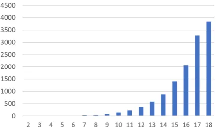
Figure 3: Average number of gCM sentences (y-axis) vs mean input sentence length (x-(y-axis)

English-Spanish CM tweets for testing our mod-els which was released during the language la-beling shared task at the Workshop on “Compu-tational Approaches to Code-switching, EMNLP 2014” (Solorio et al.,2014). We mixed the train-ing, validation and test datasets released during this shared task to construct a set of 13K tweets, which we shall refer to as Test-14. The two test datasets are tweets that were collected three years apart, and therefore, will help us estimate the ro-bustness of the language models. As shown in Ta-ble 1, these datasets are quite different in terms of CMI and average number of SP per tweet. For computing the CMI and SP, we used a English-Spanish LID to language tag the words. In fact, 9500 tweets in the Test-14 dataset are monolin-gual, but we chose to retain them because it re-flects the real distribution of CM data. Further, Test-14 also has manually annotated language la-bels, which will be helpful while conducting an in-depth analysis of the models.

3.3 Synthetic Code-Mixed Data

As described in the previous section, we use par-allel monolingual sentences to generate grammat-ically valid code mixed sentences. The entire pro-cess involves the following four steps.

Step 1: We created the parallel corpus by gen-erating translations for all the monolingual En-glish and Spanish tweets (4.5M each) using the Bing Translator API.2 We have found, that the translation quality varies widely across different sentences. Thus, we rank the translated sen-tences using Pseudo Fuzzy-match Score (PFS)

2

(He et al., 2010). First, the forward translation engine (eg. English-to-Spanish) translates mono-lingual source sentences into targett. Then the reverse translation system (eg. Spanish-English) translates target t into pseudo source s0. Equa-tion2computes the PFS betweensands0.

P F S= EditDistance(s, s 0₎

max(|s|,|s0_|) (2)

After manual inspection, we decided to select translation pairs whoseP F S ≤0.7. The edit dis-tance is based onWagner and Fischer(1974).

Step 2: We used the fast align toolkit3 (Dyer et al., 2013), to generate the word align-ments from these parallel sentences.

Step 3: The constituency parses for all the English tweets were obtained using the Stanford PCFG parser (Klein and Manning,2003).

Step 4:Using the parallel sentences, alignments and parse trees, we apply the Equivalent constraint theory (Sec2.2) to generate all syntactically valid CM sentences while allowing for lexical substitu-tion.

We randomly selected 50K monolingual Span-ish and EnglSpan-ish tweets whose PFS ≤ 0.7. This gave us 200K monolingual tweets in all (Mono dataset) and the total amount of generated CM sentences from these 100K translation pairs was 31M, which we shall refer to as gCM. Note that even though we consider the Mono and gCM as two separate sets, in reality the EC model also generates the monolingual sentences; further, existence of gCM presumes existence of Mono. Hence, we also use Mono as part of all training experiments which usegCM.

We would also like to point out that the choice of experimenting with a much smaller set of tweets, only 50K per language, was made because the number of generated tweets even from this small set of monolingual tweet pairs is almost pro-hibitively large to allow experimentation with sev-eral models and their respective configurations.

4 Approach

Language modeling is a very widely researched topic (Rosenfeld,2000;Bengio et al.,2003; Sun-dermeyer et al.,2015). In recent times, deep learn-ing has been successfully employed to build ef-ficient LMs (Mikolov et al., 2010;Sundermeyer et al.,2012;Arisoy et al.,2012;Che et al.,2017).

3_{https://github.com/clab/fast align}

Baheti et al.(2017) recently showed that there is significant effect of the training curriculum, that is the order in which data is presented to an RNN-based LM, on the perplexity of the learnt English-Spanish CM language model on tweets. Along similar lines, in this study we focus our experi-ments on training curriculum, especially regarding the use of gCM data during training, which is the primary contribution of this paper.

We do not attempt to innovate in terms of the architecture or computational structure of the LM, and use a standard LSTM-based RNN LM ( Sun-dermeyer et al.,2012) for all our experiments. In-deed, there are enough reasons to believe that CM language is not fundamentally different from non-CM language, and therefore, should not require an altogether different LM architecture. Rather, the difference arises in terms of added complexity due to the presence of lexical items and syntactic struc-tures from two linguistic systems that blows up the space of valid grammatical and lexical configura-tions, which makes it essential to train the models on large volumes of data.

4.1 Training Curricula

Baheti et al. (2017) showed that rather than ran-domly mixing the monolingual and CM data dur-ing traindur-ing, the best performance is achieved when the LM is first trained with a mixture of monolingual texts from both languages in nearly equal proportions, and ending with CM data. Mo-tivated by this finding, we define the following ba-sic training curricula (“X | Y” indicates training the model first with data X and then data Y):

(1)rCM,(2)Mono,(3)Mono|rCM, (4a)Mono|gCM,(4b)gCM|Mono, (5a)Mono|gCM|rCM,

(5b)gCM|Mono|rCM

Curricula 1-3 are baselines, where gCM data is not used. Note that curriculum 3 is the best case according toBaheti et al.(2017). Curricula 4a and 4b help us examine how far generated data can substitute real data. Finally, curricula 5a and 5b use all the data, and we would expect them to per-form the best.

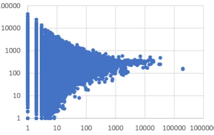
Figure 4: Scatter plot of fractional increase in word frequency in gCM (y-axis) vs original fre-quency (x-axis).

4.2 Sampling from gCM

As we have seen in Sec 3.3 (Fig. 3), in the EC model, a pair of monolingual parallel tweets gives rise to a large number (typically exponential in the length of the tweet) of CM tweets. On the other hand, in reality, only a few of those tweets would be observed. Further, if all the generated sentences are used to train an LM, it is not only computation-ally expensive, it also leads to undesirable results because the statistical properties of the distribution of the gCM corpus is very different from real data. We see this in our experiments (not reported in this paper for paucity of space), and also in Fig4, where we plot the ratio of the frequencies of the words ingCMandMonocorpora (y-axis) against their original frequencies in Mono (x-axis). We can clearly see that the frequencies of the words are scaled up non-uniformly, the ratios varying be-tween 1 and 500,000 for low frequency words.

In order to reduce this skew, instead of select-ing the entire gCM data, we propose three sam-pling techniques for creating the training data from gCM:

Random: For each monolingual pair of parallel tweets, we randomly pick a fixed number, k, of CM tweets. We shall refer to the resultant training corpus asχ-gCM.

CMI-based: For each monolingual pair of par-allel tweets, we randomly pickk CM tweets and bucket them using CMI (in 0.1 intervals). Thus, in this case we can define two different curric-ula, where we present the data in increasing or decreasing order of CMI during training, which will be represented by the notations ↑-gCM and

↓-gCMrespectively.

SPF-based: For each monolingual pair of par-allel tweets, we randomly pickkCM tweets such that the SPF distribution (section 3.1) of these tweets is similar to that of rCM data (as estimated from the validation set). This strategy will be re-ferred to asρ-gCM.

Thus, depending on the gCM sampling strategy used, curricula 4a-b and 5a-b can have three differ-ent versions each. Note that since CMI forMono is 0, ↑-gCMis not meaningful for 4b and 5b and similarly,↓-gCMnot for 4a and 5a.

5 Experiments and Results

For all our experiments, we use a 2 layered RNN with LSTM units and hidden layer dimension of 100. While training, we use sampled softmax with 5000 samples instead of a full softmax to speed up the training process. The sampling is based on the word frequency in the training corpus. We use momentum SGD with a learning rate of 0.002. We have used the CNTK toolkit for building our mod-els.4 We use a fixed k=5 (from each monolingual pair) for sampling the gCM data. We observed the performance on↑-gCM to be the best when trained till CMI 0.4 and similarly on↓-gCM when trained from 1.0 to 0.6.

5.1 Results

Table 2 presents the perplexities on validation, Test-14 and Test-17 datasets for all the models (Col. 3, 4 and 5). We observe the following trends: (1) Model 5(b)-ρ has the least perplex-ity value (significantly different from the second lowest value in the column, p < 0.00001 for a paired t-test). (2) There is 55 and 90 point re-duction in perplexity on Test-17 and Test-14 sets respectively from the baseline experiment 3, that does not use gCM data. Thus, addition of gCM data is helpful. (3) Only the 4a and 4b models are worse than 3, while 5a and 5b models are better. Hence, rCM is indispensable, even though gCM helps. (4) SPF based sampling performs signifi-cantly better (againp <0.00001) than other sam-pling techniques.

To put these numbers in perspective, we also trained our model on 50k monolingual English data, which gave a PPL of 264. This shows that the high PPL values our models obtain are due to the inherent complexity of modeling CM lan-guage. This is further substantiated by the PPL

ID Training curriculum Overall PPL Avg. SP PPL

Valid Test-17 Test-14 Valid Test-17 Test-14

1 rCM 1995 2018 1822 5598 5670 8864

2 Mono 1588 1607 892 23378 23790 26901

3 Mono|rCM 1029 1041 861 4734 4824 7913

4(a)-χ Mono|χ-gCM 1749 1771 1119 5752 5869 6065

4(a)-↑ Mono| ↑-gCM 1852 1872 1208 9074 9167 8803

4(a)-ρ Mono|ρ-gCM 1599 1618 1116 6534 6618 7293

4(b)-χ χ-gCM|Mono 1659 1680 903 20634 21028 20300

4(b)-↓ ↓-gCM|Mono 1900 1917 973 28422 28722 25006

4(b)-ρ ρ-gCM|Mono 1622 1641 871 26191 26710 22557

5(a)-χ Mono|χ-gCM|rCM 1026 1038 836 4317 4386 5958

5(a)-↑ Mono| ↑-gCM|rCM 1045 1058 961 4983 5078 6861

5(a)-ρ Mono|ρ-gCM|rCM 999 1011 830 4736 4829 6807

5(b)-χ χ-gCM|Mono|rCM 1006 1019 790 4878 4987 7018

5(b)-↓ ↓-gCM|Mono|rCM 1012 1025 800 5396 5489 7476

5(b)-ρ ρ-gCM|Mono|rCM 976 986 772 4810 4912 6547

Table 2: Perplexity of the LM Models on all tweets and only on SP (right block).

RL 3 5(a)-χ 5(a)-ρ 5(a)-↑ 5(b)-↓ 5(b)-χ 5(b)-ρ

1 13222 12815 13717 14017 13761 13494 13077 2 2201 2120 2064 2078 2155 2256 2108 3 970 926 902 896 914 966 911 4 643 594 567 575 573 608 571

5 574 540 509 517 502 553 503

6 593 545 529 543 520 566 529

≥7 507 465 444 460 431 479 440

Table 3: Perplexities of minor language runs for various run lengths on Test-17.

# rCM 0.5K 1K 2.5K 5K 10K 50K

3 1238 1186 1120 1041 991 812

5(b)-ρ 1181 1141 1068 986 951 808

Table 4: Perplexity variation on Test-17 with changes in amount of rCM train data. Similar trends for other models (left for paucity of space)

values computed only at the code-switch points, which are shown in Table2, col. 6, 7 and 8. Even for the best model, which in this case is 5(a)-χ, PPL is four times higher than the overall PPL on Test-17.

Run length: The complexity of modeling CM is also apparent from Table 3, which reports the perplexity value of the 3 and 5 models for mono-lingual fragments of variousrun lengths. We de-finerun length as the number of words in a max-imal monolingual fragment orrunwithin a tweet. In our analysis, we only consider runs of the em-bedded language, defined as the language that has fewer words. As one would expect, model 5(a)-χperforms the best for run length 1 (recall that it has lowest PPL at SP), but as the run length in-creases, the models sampling the gCM data

us-Sample size (k) 1 2 5 10

# tweets 93K 184K 497K 952K

5(b)-ρ 1081 1053 986 1019

Table 5: Variation of PPL on Test-17 with gCM sample sizek. Similar trends for other models.

ing CMI (5(a)-↑ and 5(b)-↓) are better than the randomly sampled (χ) models. Run length 1 are typically cases of word borrowing and lexical sub-stitution; higher run length segments are typically an indication of CM. Clearly, modeling the shorter runs of the embedded language seems to be one of the most challenging aspect of CM LM.

Significance of Linguistic Constraints: To understand the importance of the linguistic con-straints imposed by EC on generation of gCM, we conducted an experiment where a synthetic CM corpus was created by combining random contigu-ous segments from the monolingual tweets such that the generated CM tweets’ SPF distribution matched that of rCM. When we replaced gCM by this corpus in5(b)-ρ, the PPL on test-17 was 1060, which is worse than the baseline PPL.

gen-eral, model 3 needs twice the amount of rCM data to perform as well as model 5(b)-ρ.

Effect of gCM size: In our sampling methods on gCM data, we fixed our sample size,kas 5 for consistency and feasibility of experiments. To un-derstand the effect ofk(and hence the size of the gCM data), we experimented withk=1, 2, and 10 keeping everything else fixed. Table5reports the results for the models 3 and 5(b)-ρ. We observe that unlike rCM data, increasing gCM data or k does not necessarily decrease PPL after a point. We speculate that there is trade-off betweenkand the amount of rCM data, and also probably be-tween these and the amount of monolingual data. We plan to explore this further in future.

6 Related Work

We briefly describe the various types of ap-proaches used for building LM for CM text.

Bilingual models: These models combine data from monolingual data sources in both languages (Weng et al., 1997). Factored models: Geb-hardt(2011) uses Factored Language Models for rescoring n-best lists during ASR decoding. The factors used include POS tags, CS point prob-ability and LID. In Adel et al.(2014b; 2014a; 2013) RNNLMs are combined with n-gram based models, or converted to backoff models, giv-ing improvements in perplexity and mixed error rate. Models that incorporate linguistic con-straints: Li and Fung(2013) use inversion con-straints to predict CS points and integrates this prediction into the ASR decoding process. Li and Fung(2014) integrates Functional Head con-straints (FHC) for code-switching into the Lan-guage Model for Mandarin-English speech recog-nition. This work uses parsing techniques to re-strict the lattice paths during decoding of speech to those permissible under the FHC theory. Our method instead imposes grammatical constraints (EC theory) to generate synthetic data, which can potentially be used to augment real CM data. This allows flexibility to deploy any sophisticated LM architecture and the synthetic data generated can also be used for CM tasks other than speech recog-nition. Training curricula for CM:Baheti et al. (2017) show that a training curriculum where an RNN-LM is trained first with interleaved monolin-gual data in both languages followed by CM data gives the best results for English-Spanish LM. The perplexity of this model is 4544, which then

re-duces to 298 after interpolation with a statistical n-gram LM. However, these numbers are not di-rectly comparable to our work because the datasets are different. Our work is an extension of this ap-proach showing that adding synthetic data further improves results.

We do not know of any work that uses syntheti-cally generated CM data for training LMs.

7 Conclusion

In this paper, we presented a computational method for generating synthetic CM data based on the EC theory of code-mixing, and showed that sampling text from the synthetic corpus (according to the distribution of SPF found in real CM data) helps in reduction of PPL of the RNN-LM by an amount which is equivalently achieved by doubling the amount of real CM data. We also showed that randomly generated CM data doesn’t improve the LM. Thus, the linguistic theory based generation is of crucial significance. There is no unanimous theory in linguistics on syntactic structure of CM language. Hence, as a future work, we would like to compare the useful-ness of different linguistic theories and different constraints within each theory in our proposed LM framework. This can also provide an indirect validation of the theories. Further, we would like to study sampling techniques motivated by natural distributions of linguistic structures.

Acknowledgements

We would like to thank the anonymous reviewers for their valuable suggestions.

References

Heike Adel, K. Kirchhoff, N. T. Vu, D. Telaar, and T. Schultz. 2014a. Combining recurrent neural net-works and factored language models during decod-ing of code-switchdecod-ing speech. InINTERSPEECH, pages 1415–1419.

Heike Adel, K Kirchhoff, N T Vu, D Telaar, and T Schultz. 2014b. Comparing approaches to con-vert recurrent neural networks into backoff language models for efficient decoding. InINTERSPEECH, pages 651–655.

Ebru Arisoy, Tara N Sainath, Brian Kingsbury, and Bhuvana Ramabhadran. 2012. Deep neural network language models. In Proceedings of the NAACL-HLT 2012 Workshop: Will We Ever Really Replace the N-gram Model? On the Future of Language Modeling for HLT, pages 20–28. Association for Computational Linguistics.

Ashutosh Baheti, Sunayana Sitaram, Monojit Choud-hury, and Kalika Bali. 2017. Curriculum design for code-switching: Experiments with language iden-tification and language modeling with deep neural networks. InProc. of ICON-2017, Kolkata, India, pages 65–74.

Utsab Barman, Amitava Das, Joachim Wagner, and Jennifer Foster. 2014. Code mixing: A challenge for language identification in the language of social media. InThe 1st Workshop on Computational Ap-proaches to Code Switching, EMNLP 2014.

Hedi M Belazi, Edward J Rubin, and Almeida Jacque-line Toribio. 1994. Code switching and x-bar the-ory: The functional head constraint. Linguistic in-quiry, pages 221–237.

Yoshua Bengio, R´ejean Ducharme, Pascal Vincent, and Christian Jauvin. 2003. A neural probabilistic lan-guage model. Journal of machine learning research, 3(Feb):1137–1155.

Tong Che, Yanran Li, Ruixiang Zhang, R Devon Hjelm, Wenjie Li, Yangqiu Song, and Yoshua Ben-gio. 2017. Maximum-likelihood augmented discrete generative adversarial networks. arXiv preprint arXiv:1702.07983.

A.-M. DiSciullo, Pieter Muysken, and R. Singh. 1986. Government and code-mixing. Journal of Linguis-tics, 22:1–24.

Chris Dyer, Victor Chahuneau, and N A. Smith. 2013. A simple, fast, and effective reparameterization of ibm model 2. InProceedings of NAACL-HLT 2013, pages 644–648. Association for Computational Lin-guistics.

B. Gamback and A Das. 2014. On measuring the com-plexity of code-mixing. InProc. of the 1st Workshop on Language Technologies for Indian Social Media (Social-India).

B. Gamback and A Das. 2016. Comparing the level of code-switching in corpora. InProc. of the 10th In-ternational Conference on Language Resources and Evaluation (LREC).

Jan Gebhardt. 2011. Speech recognition on english-mandarin code-switching data using factored lan-guage models.

Yifan He, Yanjun Ma, Andy Way, and Josef Van Gen-abith. 2010. Integrating n-best smt outputs into a tm system. InProceedings of the 23rd International Conference on Computational Linguistics: Posters, pages 374–382. Association for Computational Lin-guistics.

A. K. Joshi. 1985. Processing of Sentences with In-trasentential Code Switching. In D. R. Dowty, L. Karttunen, and A. M. Zwicky, editors, Natural Language Parsing: Psychological, Computational, and Theoretical Perspectives, pages 190–205. Cam-bridge University Press, CamCam-bridge.

D Klein and CD Manning. 2003. Accurate unlexi-calized parsing. In Proceedings of the 41st annual meeting of the association for computational lin-guistics. Association of Computational Linguistics.

Ying Li and P Fung. 2013. Improved mixed lan-guage speech recognition using asymmetric acoustic model and language model with code-switch inver-sion constraints. InICASSP, pages 7368–7372.

Ying Li and P Fung. 2014. Language modeling with functional head constraint for code switching speech recognition. InEMNLP.

Tom´aˇs Mikolov, Martin Karafi´at, Luk´aˇs Burget, Jan ˇ

Cernock`y, and Sanjeev Khudanpur. 2010. Recur-rent neural network based language model. In Eleventh Annual Conference of the International Speech Communication Association.

Carol Myers-Scotton. 1993. Duelling Lan-guages:Grammatical structure in Code-switching. Clarendon Press, Oxford.

Carol Myers-Scotton. 1995. A lexically based model of code-switching. In Lesley Milroy and Pieter Muysken, editors, One Speaker, Two Languages: Cross-disciplinary Perspectives on Code-switching, pages 233–256. Cambridge University Press, Cam-bridge.

Rana D. Parshad, Suman Bhowmick, Vineeta Chand, Nitu Kumari, and Neha Sinha. 2016. What is India speaking? Exploring the “Hinglish” invasion. Phys-ica A, 449:375–389.

Shana Poplack. 1980. Sometimes Ill start a sentence in Spanish y termino en espaol. Linguistics, 18:581– 618.

Ameya Prabhu, Aditya Joshi, Manish Shrivastava, and Vasudeva Varma. 2016. Towards sub-word level compositions for sentiment analysis of hindi-english code mixed text. InProceedings of COLING 2016, the 26th International Conference on Computational Linguistics: Technical Papers, pages 2482–2491.

Shruti Rijhwani, R Sequiera, M Choudhury, K Bali, and C S Maddila. 2017. Estimating code-switching on Twitter with a novel generalized word-level lan-guage identification technique. InACL.

Ronald Rosenfeld. 2000. Two decades of statistical language modeling: Where do we go from here? Proceedings of the IEEE, 88(8):1270–1278.

and sentiment: What do Hindi-English speakers do on Twitter? InEMNLP, pages 1131–1141.

David Sankoff. 1998. A formal production-based ex-planation of the facts of code-switching. Bilingual-ism: language and cognition, 1(01):39–50.

A. Sharma, S. Gupta, R. Motlani, P. Bansal, M. Srivas-tava, R. Mamidi, and D.M Sharma. 2016. Shallow parsing pipeline for hindi-english code-mixed social media text. InProceedings of NAACL-HLT.

Sunayana Sitaram, Sai Krishna Rallabandi, Shruti Ri-jhwani, and Alan W Black. 2016. Experiments with cross-lingual systems for synthesis of code-mixed text. In9th ISCA Speech Synthesis Workshop.

Thamar Solorio and Yang Liu. 2008. Part-of-speech tagging for english-spanish code-switched text. In Proc. of EMNLP.

Thamar Solorio et al. 2014. Overview for the first shared task on language identification in code-switched data. In 1st Workshop on Computational Approaches to Code Switching, EMNLP, pages 62– 72.

Martin Sundermeyer, Hermann Ney, and Ralf Schl¨uter. 2015. From feedforward to recurrent lstm neural networks for language modeling. IEEE Transac-tions on Audio, Speech, and Language Processing, 23(3):517–529.

Martin Sundermeyer, Ralf Schl¨uter, and Hermann Ney. 2012. Lstm neural networks for language model-ing. In Thirteenth Annual Conference of the Inter-national Speech Communication Association.

Yogarshi Vyas, S Gella, J Sharma, K Bali, and M Choudhury. 2014. POS Tagging of English-Hindi Code-Mixed Social Media Content. InProc. EMNLP, pages 974–979.

Robert A Wagner and Michael J Fischer. 1974. The string-to-string correction problem. Journal of the ACM (JACM), 21(1):168–173.