Lifelong Learning for Sentiment Classification

Lifelong Learning for Sentiment Classification

Zhiyuan Chen, Nianzu Ma, Bing Liu Department of Computer Science

University of Illinois at Chicago

{czyuanacm,jingyima005}@gmail.com,liub@cs.uic.edu

Abstract

This paper proposes a novel lifelong learn-ing (LL) approach to sentiment classifica-tion. LL mimics the human continuous learning process, i.e., retaining the knowl-edge learned from past tasks and use it to help future learning. In this paper, we first discuss LL in general and then LL for sentiment classification in particular. The proposed LL approach adopts a Bayesian optimization framework based on stochas-tic gradient descent. Our experimental re-sults show that the proposed method out-performs baseline methods significantly, which demonstrates that lifelong learning is a promising research direction.

1 Introduction

Sentiment classification is the task of classifying an opinion document as expressing a positive or negative sentiment. Liu (2012) and Pang and Lee (2008) provided good surveys of the existing re-search. In this paper, we tackle sentiment clas-sification from a novel angle, lifelong learning

(LL), or lifelong machine learning. This learn-ing paradigm aims to learn as humans do: re-taining the learned knowledge from the past and use the knowledge to help future learning (Thrun, 1998, Chen and Liu, 2014b, Silver et al., 2013).

Although many machine learning topics and techniques are related to LL, e.g., lifelong learn-ing (Thrun, 1998, Chen and Liu, 2014b, Silver et al., 2013), transfer learning (Jiang, 2008, Pan and Yang, 2010), multi-task learning (Caruana, 1997), never-ending learning (Carlson et al., 2010), self-taught learning (Raina et al., 2007), and online learning (Bottou, 1998), there is still no unified definition for LL.

Based on the prior work and our research, to build an LL system, we believe that we need to answer the following key questions:

1. What information should be retained from the past learning tasks?

2. What forms of knowledge will be used to help future learning?

3. How does the system obtain the knowledge? 4. How does the system use the knowledge to help

future learning?

Motivated by these questions, we present the following definition oflifelong learning(LL).

Definition (Lifelong Learning): A learner has performed learning on a sequence of tasks, from 1 toN−1. When faced with theNth task, it uses the knowledge gained in the pastN −1tasks to help learning for theNth task. An LL system thus needs the following four general components: 1. Past Information Store (PIS): It stores the

in-formation resulted from the past learning. This may involve sub-stores for information such as (1) the original data used in each past task, (2) intermediate results from the learning of each past task, and (3) the final model or patterns learned from the past task, respectively. 2. Knowledge Base(KB): It stores the knowledge

mined or consolidated from PIS (Past Informa-tion Store). This requires a knowledge repre-sentation scheme suitable for the application. 3. Knowledge Miner (KM). It mines knowledge

from PIS (Past Information Store). This min-ing can be regarded as a meta-learnmin-ing process because it learns knowledge from information resulted from learning of the past tasks. The knowledge is stored to KB (Knowledge Base). 4. Knowledge-Based Learner (KBL): Given the

knowledge in KB, this learner is able to lever-age the knowledge and/or some information in PIS for the new task.

Based on this, we can definelifelong sentiment classification(LSC):

Definition (Lifelong Sentiment Classification): A learner has performed a sequence of supervised

sentiment classification tasks, from 1 to N −1, where each task consists of a set of training doc-uments with positive and negative polarity labels. Given theNth task, it uses the knowledge gained in the pastN −1tasks to learn a better classifier for theNth task.

It is useful to note that although many re-searchers have used transfer learning for super-vised sentiment classification, LL is different from the classic transfer learning or domain adapta-tion (Pan and Yang, 2010). Transfer learning typi-cally uses labeled training data from one (or more) source domain(s) to help learning in the target do-main that has little or no labeled data (Aue and Gamon, 2005, Bollegala et al., 2011). It does not use the results of the past learning or knowledge mined from the results of the past learning. Fur-ther, transfer learning is usually inferior to tradi-tional supervised learning when the target domain already has good training data. In contrast, our target (or future) domain/task has good training data and we aim to further improve the learning using both the target domain training data and the knowledge gained in past learning. To be consis-tent with prior research, we treat the classification of one domain as one learning task.

One question is why the past learning tasks can contribute to the target domain classification given that the target domain already has labeled training data. The key reason is that the training data may not be fully representative of the test data due to the sample selection bias (Heckman, 1979, Shi-modaira, 2000, Zadrozny, 2004). In few real-life applications, the training data are fully represen-tative of the test data. For example, in a senti-ment classification application, the test data may contain some sentiment words that are absent in the training data of the target domain, while these sentiment words have appeared in some past do-mains. So the past domain knowledge can provide the prior polarity information in this situation.

Like most existing sentiment classification pa-pers (Liu, 2012), this paper focuses on binary clas-sification, i.e., positive (+) and negative (−) polar-ities. But the proposed method is also applicable to multi-class classification. To embed and use the knowledge in building the target domain classifier, we propose a novel optimization method based on the Na¨ıve Bayesian (NB) framework and stochas-tic gradient descent. The knowledge is incorpo-rated using penalty terms in the optimization

for-mulation. This paper makes three contributions: 1. It proposes a novel lifelong learning approach

to sentiment classification, calledlifelong sen-timent classification(LSC).

2. It proposes an optimization method that uses penalty terms to embed the knowledge gained in the past and to deal with domain dependent sentiment words to build a better classifier. 3. It creates a large corpus containing reviews

from 20 diverse product domains for extensive evaluation. The experimental results demon-strate the superiority of the proposed method.

2 Related Work

Our work is mainly related to lifelong learning and multi-task learning (Thrun, 1998, Caruana, 1997, Chen and Liu, 2014b, Silver et al., 2013). Existing lifelong learning approaches focused on exploiting invariances (Thrun, 1998) and other types of knowledge (Chen and Liu, 2014b, Chen and Liu, 2014a, Ruvolo and Eaton, 2013) across multiple tasks. Multi-task learning optimizes the learning of multiple related tasks at the same time (Caruana, 1997, Chen et al., 2011, Saha et al., 2011, Zhang et al., 2008). However, these meth-ods are not for sentiment analysis. Also, our na¨ıve Bayesian optimization based LL method is quite different from all these existing techniques.

3 Proposed LSC Technique

3.1 Na¨ıve Bayesian Text Classification

Before presenting the proposed method, we briefly review the Na¨ıve Bayesian (NB) text classification as our method uses it as the foundation.

NB text classification (McCallum and Nigam, 1998) basically computes the conditional proba-bility of each word w given each class cj (i.e.,

P(w|cj)) and the prior probability of each class

cj (i.e., P(cj)), which are used to calculate the posterior probability of each classcj given a test document d (i.e., P(cj|d)). cj is either positive (+) or negative (−) in our case.

The key parameterP(w|cj)is computed as:

P(w|cj) = λ+Ncj,w

λ|V|+P|_vV₌₁| Ncj,v

(1)

whereNcj,w is the frequency of wordwin

docu-ments of classcj. |V|is the size of vocabularyV andλ(0≤λ≤1) is used for smoothing.

3.2 Components in LSC

This subsection describes our proposed method corresponding to the proposed LL components. 1. Past Information Store (PIS): In this work, we

do not store the original data used in the past learning tasks, but only their results. For each past learning tasktˆ, we store a) Pˆt_{(w|+) and}

Pˆt_{(w|−)for each wordwwhich are from task}

ˆ

t’s NB classifier (see Eq 1); and b) the number of times thatw appears in a positive (+) doc-ument Nˆt

+,w and the number of times that w appears in a negative documentsNtˆ

−,w.

2. Knowledge Base (KB): Our knowledge base contains two types of knowledge:

(a) Document-level knowledge NKB

+,w (and

NKB

−,w): number of occurrences of w in the documents of the positive (and nega-tive) class in the past tasks, i.e., NKB

+,w =

P

ˆ

tN+ˆt,wandN−KB,w =PˆtN−ˆt,w. (b) Domain-level knowledge MKB

+,w (and

MKB

−,w): number of past tasks in which P(w|+) > P(w|−) (and

P(w|+)< P(w|−)).

3. Knowledge Miner (KM). Knowledge miner is straightforward as it just performs counting and aggregation of information in PIS to generate knowledge (see 2(a) and 2(b) above).

4. Knowledge-Based Learner (KBL): This learner incorporates knowledge using regularization as

penalty terms in our optimization. See the de-tails in 3.4.

3.3 Objective Function

In this subsection, we introduce the objective func-tion used in our method. The key parameters that affect NB classification results areP(w|cj)which are computed using empirical counts of word w

with classcj, i.e.,Ncj,w(Eq. 1). In binary

classifi-cation, they are N+,w and N−,w. This suggests that we can revise these counts appropriately to improve classification. In our optimization, we denote the optimized variables X+,w and X−,w as the number of times that a word wappears in the positive and negative class. We called them

virtual countsto distinguish them from empirical countsN+,wandN−,w. For correct classification, ideally, we should have the posterior probability

P(cj|di) = 1for labeled classcj, and for the other classcf, we should haveP(cf|di) = 0. Formally, given a new domain training dataDt_{, our objective} function is:

|Dt_| X

i=1

(P(cj|di)−P(cf|di)) (2)

Herecj is the actual labeled class ofdi ∈ Dt. In this paper, we use stochastic gradient descent (SGD) to optimize on the classification of each document di ∈ Dt. Due to the space limit, we only show the optimization process for a positive document (the process for a negative document is similar). The objective function under SGD for a positive document is:

F+,i=P(+|di)−P(−|di) (3) To further save space, we omit the derivation steps and give the final derivatives below (See the detailed derivation steps in the separate supple-mentary note):

g(X) = λ|V|+ P|V|

v=1X+,v

λ|V|+P|V|

v=1X−,v

!|d_i|

(4)

∂F+,i

∂X+,u = n_u,di λ+X+,u+

P(−)

P(+) Q

w∈di

λ+X−,w

λ+X+,w nw,di

× ∂g ∂X+,u 1 +P(−)

P(+) Q

w∈di

λ+X−,w

λ+X+,w nw,di

×g(X) − nu,di

λ+X+,u

(5)

∂F+,i

∂X−,u =

n_u,di

λ+X−,u ×g(X) +

∂g ∂X−,u

P(+)

P(−) Q

w∈di

λ+X+,w

λ+X−,w

n_w,di

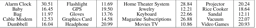
Alarm Clock 30.51 Flashlight 11.69 Home Theater System 28.84 Projector 20.24

Baby 16.45 GPS 19.50 Jewelry 12.21 Rice Cooker 18.64

Bag 11.97 Gloves 13.76 Keyboard 22.66 Sandal 12.11

Cable Modem 12.53 Graphics Card 14.58 Magazine Subscriptions 26.88 Vacuum 22.07 Dumbbell 16.04 Headphone 20.99 Movies TV 10.86 Video Games 20.93 Table 1: Names of the 20 product domains and the proportion of negative reviews in each domain.

wherenu,di is the term frequency of worduin

documentdi. X denotes all the variables consist-ing ofX+,wandX−,wfor each wordw. The par-tial derivatives for a wordu, i.e.,_∂X∂g_+,u and_∂X∂g_−,u, are quite straightforward and thus not shown here.

X0

+,w =N+t,w+N+KB,wandX−0,w =N−t,w+N−KB,w are served as a reasonable starting point for SGD, whereNt

+,wandN−t,ware the empirical counts of wordwand classes+and−from domainDt_{, and}

NKB

+,w andN−KB,w are from knowledge KB (Sec-tion 3.2). The SGD runs iteratively using the fol-lowing rules for the positive document di until convergence, i.e., when the difference of Eq. 2 for two consecutive iterations is less than1e−3(same for the negative document), whereγis the learning rate:

X₊l_,u =X₊l−_,u1−γ_∂X∂F+,i +,u, X

l

−,u=X−l−,u1−γ_∂X∂F+,i

−,u

3.4 Exploiting Knowledge via Penalty Terms

The above optimization is able to update the vir-tual counts for a better classification in the target domain. However, it does not deal with the issue of domain dependent sentiment words, i.e., some words may change the polarity across different do-mains. Nor does it utilize the domain-level knowl-edge in the knowlknowl-edge baseKB(Section 3.2). We thus propose to add penalty terms into the opti-mization to accomplish these.

The intuition here is that if a word w can dis-tinguish classes very well from the target domain training data, we should rely more on the target domain training data in computing counts related tow. So we define a set of wordsVT that consists of distinguishable target domain dependent words. A wordwbelongs toVT ifP(w|+)is much larger or much smaller than P(w|−) in the target do-main, i.e., _PP(₍w_w|_|−+)₎ ≥ σ or _PP(₍w_w|−_|+)) ≥ σ, whereσ

is a parameter. Such words are already effective in classification for the target domain, so the vir-tual counts in optimization should follow the em-pirical counts (Nt

+,w andN−t,w) in the target do-main, which are reflected in the L2 regularization penalty term below (αis the regularization coeffi-cient):

1 2α

X

w∈VT

X+,w−N+t,w2+ X−,w−N−t,w2

(7)

To leverage domain-level knowledge (the sec-ond type of knowledge inKB in Section 3.2), we want to utilize only those reliable parts of knowl-edge. The rationale here is that if a word only appears in one or two past domains, the knowl-edge associated with it is probably not reliable or it is highly specific to those domains. Based on it, we use domain frequency to define the relia-bility of the domain-level knowledge. For w, if

MKB

+,w ≥ τ orM−KB,w ≥ τ (τ is a parameter), we regard it as appearing in a reasonable number of domains, making its knowledge reliable. We de-note the set of such words asVS. Then we add the second penalty term as follows:

1 2α

X

w∈VS

X+,w−Rw×X+0,w2

+1₂α X

w∈VS

X−,w−(1−Rw)×X−0,w2 (8)

where the ratioRw is defined asM+KB,w/(M+KB,w +

MKB

−,w).X+0,wandX−0,ware the starting points for SGD (Section 3.3). Finally, we revise the partial derivatives in Eqs. 4-6 by adding the correspond-ing partial derivatives of Eqs. 7 and 8 to them.

4 Experiments

Datasets. We created a large corpus contain-ing reviews from 20 types of diverse products or domains crawled from Amazon.com (i.e., 20 datasets). The names of product domains are listed in Table 1. Each domain contains 1,000 views. Following the existing work of other re-searchers (Blitzer et al., 2007, Pang et al., 2002), we treat reviews with rating >3 as positive and reviews with rating<3 as negative. The datasets are publically available at the authors websites.

NB-T NB-S NB-ST SVM-T SVM-S SVM-ST CLF LSC

56.21 57.04 60.61 57.82 57.64 61.05 12.87 67.00

Table 2: Natural class distribution: Average F1-score of the negative class over 20 domains. Negative class is the minority class and thus harder to classify.

NB-T NB-S NB-ST SVM-T SVM-S SVM-ST CLF LSC

80.15 77.35 80.85 78.45 78.20 79.40 80.49 83.34

Table 3: Balanced class distribution: Average accuracy over 20 domains for each system.

Balanced class distribution: We also created a balance dataset with 200 reviews (100 positive and 100 negative) in each domain dataset. This set is smaller because of the small number of negative reviews in each domain. Accuracy is used for eval-uation in this balanced setting.

We used unigram features with no feature se-lection in classification. We followed (Pang et al., 2002) to deal with negation words. For evalua-tion, each domain is treated as the target domain with the rest 19 domains as the past domains. All the models are evaluated using 5-fold cross vali-dation.

Baselines. We compare our proposed LSC model with Na¨ıve Bayes (NB), SVM1_{, and} CLF (Li and Zong, 2008). Note that NB and SVM can only work on a single domain data. To have a comprehensive comparison, they are fed with three types of training data:

a) labeled training data from the target domain only, denoted by NB-T and SVM-T;

b) labeled training data from all past source do-mains only, denoted by NB-S and SVM-S; c) merged (labeled) training data from all past

do-mains and the target domain, referred to as NB-ST and SVM-NB-ST.

For LSC, we empirically setσ = 6andτ = 6. The learning rateλand regularization coefficient

α are set to 0.1 empirically. λ is set to 1 for (Laplace) smoothing.

Table 2 shows the average F1-scores for the negative class in the natural class distribution, and Table 3 shows the average accuracies in the bal-anced class distribution. We can clearly see that our proposed model LSC achieves the best perfor-mance in both cases. In general, NB-S (and SVM-S) are worse than NB-T (and SVM-T), both of which are worse than NB-ST (and SVM-ST). This shows that simply merging both past domains and the target domain data is slightly beneficial. Note

1_{http://www.csie.ntu.edu.tw/˜cjlin/libsvm/}

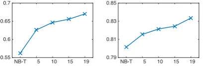
NB-T 5 10 15 19 0.79

0.81 0.83 0.85

NB-T 5 10 15 19 0.55

0.6 0.65 0.7

Figure 1: (Left): Negative class F1-score of LSC with #past domains in natural class distribution. (Right): Accuracy of LSC with #past domains in balanced class distribution.

that the average F1-score for the positive class is not shown as all classifiers perform very well be-cause the positive class is the majority class (while our model performs slightly better than the base-lines). The improvements of the proposed LSC model over all baselines in both cases are statisti-cally significant using paired t-test (p <0.01 com-pared to NB-ST and CLF,p < 0.0001compared to the others). In the balanced class setting (Ta-ble 3), CLF performs better than NB-T and SVM-T, which is consistent with the results in (Li and Zong, 2008). However, it is still worse than our LSC model.

Effects of #Past Domains. Figure 1 shows the effects of our model using different number of past domains. We clearly see that LSC performs bet-ter with more past domains, showing it indeed has the ability to accumulate knowledge and use the knowledge to build better classifiers.

5 Conclusions

References

Alina Andreevskaia and Sabine Bergler. 2008. When Specialists and Generalists Work Together: Over-coming Domain Dependence in Sentiment Tagging. InACL, pages 290–298.

Anthony Aue and Michael Gamon. 2005. Customiz-ing Sentiment Classifiers to New Domains: A Case Study. InRANLP.

John Blitzer, Mark Dredze, and Fernando Pereira. 2007. Biographies, Bollywood, Boom-boxes and Blenders: Domain Adaptation for Sentiment Clas-sification. InACL, pages 440–447.

Danushka Bollegala, David J Weir, and John Carroll. 2011. Using Multiple Sources to Construct a Sen-timent Sensitive Thesaurus for Cross-Domain Senti-ment Classification. InACL HLT, pages 132–141.

L´eon Bottou. 1998. Online algorithms and stochas-tic approximations. In David Saad, editor, Online Learning and Neural Networks. Cambridge Univer-sity Press, Cambridge, UK. Oct 2012.

Andrew Carlson, Justin Betteridge, and Bryan Kisiel. 2010. Toward an Architecture for Never-Ending Language Learning. InAAAI, pages 1306–1313.

Rich Caruana. 1997. Multitask Learning. Machine learning, 28(1):41–75.

Zhiyuan Chen and Bing Liu. 2014a. Mining Topics in Documents : Standing on the Shoulders of Big Data. InKDD, pages 1116–1125.

Zhiyuan Chen and Bing Liu. 2014b. Topic Modeling using Topics from Many Domains, Lifelong Learn-ing and Big Data. InICML, pages 703–711.

Jianhui Chen, Jiayu Zhou, and Jieping Ye. 2011. Inte-grating low-rank and group-sparse structures for ro-bust multi-task learning. InKDD, pages 42–50.

Yulan He, Chenghua Lin, and Harith Alani. 2011. Au-tomatically Extracting Polarity-Bearing Topics for Cross-Domain Sentiment Classification. In ACL, pages 123–131.

James J Heckman. 1979. Sample selection bias as a specification error. Econometrica: Journal of the econometric society, pages 153–161.

Jing Jiang. 2008. A literature survey on domain adap-tation of statistical classifiers. Technical report.

Lun-Wei Ku, Ting-Hao Huang, and Hsin-Hsi Chen. 2009. Using morphological and syntactic structures for Chinese opinion analysis. In EMNLP, pages 1260–1269.

Shoushan Li and Chengqing Zong. 2008. Multi-domain sentiment classification. InACL HLT, pages 257–260.

Fangtao Li, Sinno Jialin Pan, Ou Jin, Qiang Yang, and Xiaoyan Zhu. 2012. Cross-domain Co-extraction of Sentiment and Topic Lexicons. InACL, pages 410– 419.

Shoushan Li, Yunxia Xue, Zhongqing Wang, and Guodong Zhou. 2013. Active learning for cross-domain sentiment classification. In AAAI, pages 2127–2133.

Bing Liu. 2012. Sentiment Analysis and Opinion Min-ing. Synthesis Lectures on Human Language Tech-nologies, 5(1):1–167.

Sinno Jialin Pan and Qiang Yang. 2010. A Survey on Transfer Learning. IEEE Trans. Knowl. Data Eng., 22(10):1345–1359.

Bo Pang and Lillian Lee. 2008. Opinion mining and sentiment analysis. Foundations and Trends in In-formation Retrieval, 2(1-2):1–135.

Bo Pang, Lillian Lee, and Shivakumar Vaithyanathan. 2002. Thumbs up? Sentiment Classification using Machine Learning Techniques. In EMNLP, pages 79–86.

Rajat Raina, Alexis Battle, Honglak Lee, Benjamin Packer, and Andrew Y Ng. 2007. Self-taught Learn-ing : Transfer LearnLearn-ing from Unlabeled Data. In

ICML, pages 759–766.

Paul Ruvolo and Eric Eaton. 2013. ELLA: An efficient lifelong learning algorithm. In ICML, pages 507– 515.

Avishek Saha, Piyush Rai, Suresh Venkatasubrama-nian, and Hal Daume. 2011. Online learning of multiple tasks and their relationships. InAISTATS, pages 643–651.

Hidetoshi Shimodaira. 2000. Improving predictive in-ference under covariate shift by weighting the log-likelihood function. Journal of statistical planning and inference, 90(2):227–244.

Daniel L Silver, Qiang Yang, and Lianghao Li. 2013. Lifelong Machine Learning Systems: Beyond Learning Algorithms. InAAAI Spring Symposium: Lifelong Machine Learning, pages 49–55.

Songbo Tan, Gaowei Wu, Huifeng Tang, and Xueqi Cheng. 2007. A novel scheme for domain-transfer problem in the context of sentiment analysis. In

CIKM, pages 979–982.

Sebastian Thrun. 1998. Lifelong Learning Algo-rithms. In S Thrun and L Pratt, editors, Learning To Learn, pages 181–209. Kluwer Academic Pub-lishers.

Rui Xia and Chengqing Zong. 2011. A POS-based Ensemble Model for Cross-domain Sentiment Clas-sification. InIJCNLP, pages 614–622. Citeseer. Yasuhisa Yoshida, Tsutomu Hirao, Tomoharu Iwata,

Masaaki Nagata, and Yuji Matsumoto. 2011. Transfer Learning for Multiple-Domain Sen-timent Analysis-Identifying Domain Depen-dent/Independent Word Polarity. In AAAI, pages 1286–1291.

Bianca Zadrozny. 2004. Learning and evaluating clas-sifiers under sample selection bias. InICML, page 114. ACM.