Simple Learning and Compositional Application of Perceptually
Grounded Word Meanings for Incremental Reference Resolution
Casey Kennington CITEC, Bielefeld University
Universit¨atsstraße 25 33615 Bielefeld, Germany
ckennington@cit-ec. uni-bielefeld.de
David Schlangen CITEC, Bielefeld University
Universit¨atsstraße 25 33615 Bielefeld, Germany
david.schlangen@ uni-bielefeld.de
Abstract
An elementary way of using language is to refer to objects. Often, these objects are physically present in the shared envi-ronment and reference is done via men-tion of perceivable properties of the ob-jects. This is a type of language use that is modelled well neither by logical semantics nor by distributional semantics, the former focusing on inferential relations between expressed propositions, the latter on simi-larity relations between words or phrases. We present an account of word and phrase meaning that is perceptually grounded, trainable, compositional, and ‘dialogue-plausible’ in that it computes meanings word-by-word. We show that the approach performs well (with an accuracy of 65% on a 1-out-of-32 reference resolution task) on direct descriptions and target/landmark descriptions, even when trained with less than 800 training examples and automati-cally transcribed utterances.
1 Introduction
The most basic, fundamental site of language use is co-located dialogue (Fillmore, 1975; Clark, 1996) and referring to objects, as in Example (1), is a common occurrence in such a co-located set-ting.
(1) The green book on the left next to the mug.
Logical semantics (Montague, 1973; Gamut, 1991; Partee et al., 1993) has little to say about this process – its focus is on the construction of syntactically manipulable objects that model infer-ential relations; here, e.g. the inference that there are (at least) two objects. Vector space approaches to distributional semantics (Turney and Pantel, 2010) similarly focuses on something else, namely
semantic similarity relations between words or phrases (e.g. finding closeness for “coloured tome on the right of the cup”). Neither approach by it-self says anything about processing; typically, the assumption in applications is that fully presented phrases are being processed.
Lacking in these approaches is a notion of
grounding of symbols in features of the world (Harnad, 1990).1 In this paper, we present an
ac-count of word and phrase meaning that is (a) per-ceptually grounded in that it provides a link be-tween words and (computer) vision features of real images, (b) trainable, as that link is learned from examples of language use, (c) compositional in that the meaning of phrases is a function of that of its parts and composition is driven by structural analysis, and (d) ‘dialogue-plausible’ in that it computes meanings incrementally, word-by-word and can work with noisy input from an automatic speech recogniser (ASR). We show that the ap-proach performs well (with an accuracy of 65% on a reference resolution task out of 32 objects) on direct descriptions as well as target/landmark de-scriptions, even when trained with little data (less than 800 training examples).
In the following section we will give a back-ground on reference resolution, followed by a de-scription of our model. We will then describe the data we used and explain our evaluations. We fin-ish by giving results, providing some additional analysis, and discussion.
2 Background: Reference Resolution
Reference resolution (RR) is the task of resolving referring expressions (REs; as in Example (1)) to areferent, the entity to which they are intended to refer. Following Kennington et al. (2015a), this can be formalised as a function frr that, given a
representationU of theREand a representationW
1But see discussion below of recent extensions of these
approaches taking this into account.
of the (relevant aspects of the) world, returns I∗,
the identifier of one the objects in the world that is the referent of theRE. A number of recent papers have used stochastic models for frr where, given
W andU, a distribution over a specified set of can-didate entities inW is obtained and the probabil-ity assigned to each entprobabil-ity represents the strength of belief that it is the referent. The referent is then the argmax:
I∗ = argmax
I P(I|U, W) (1)
Recently, generative approaches, including our own, have been presented (Funakoshi et al., 2012; Kennington et al., 2013; Kennington et al., 2014; Kennington et al., 2015b; Engonopoulos et al., 2013) which model U as words or ngrams and the worldW as a set of objects in a virtual game board, represented as a set properties or concepts (in some cases, extra-linguistic or discourse as-pects were also modelled in W, such as deixis). In Matuszek et al. (2014),W was represented as a distribution over properties of tangible objects and Uwas a Combinatory Categorical Grammar parse. In all of these approaches, the objects are distinct and represented via symbolically specified prop-erties, such as colour and shape. The set of prop-erties is either read directly from the world if it is virtual, or computed (i.e., discretised) from the real world objects.
In this paper, we learn a mapping from W to Udirectly, without mediating symbolic properties; such a mapping is a kind of perceptual ground-ing of meanground-ing between W and U. Situated RR is a convenient setting for learning perceptually-grounded meaning, as objects that are referred to are physically present, are described by the RE, and have visual features that can be computation-ally extracted and represented.
Further comparison to related work will be dis-cussed in Section 5.
3 Modelling Reference to Visible Objects Overview As a representative of the kind of model explained above with formula (1), we want our model to compute a probability distribution over candidate objects, given a RE(or rather, pos-sibly just a prefix of it). We break this task down into components: The basis of our model is a model of word meaning as a function from per-ceptual features of a given object to a judgement
about how well a word and that object “fit to-gether”. (See Section 5 for discussion of prior uses of this “words as classifiers”-approach.) This can (loosely) be seen as corresponding to the inten-sionof a word, which for example in Montague’s approach is similarly modelled as a function, but from possible worlds to extensions (Gamut, 1991). We model two different types of words / word meanings: those picking out properties of single objects (e.g., “green” in “the green book”), follow-ing Kennfollow-ington et al. (2015a), and those pickfollow-ing out relations of two objects (e.g., “next to” in (1)), going beyond Kennington et al. (2015a). These word meanings are learned from instances of lan-guage use.
The second component then is the application of these word meanings in the context of an actual reference and within a phrase. This application gives the desired result of a probability distribu-tion over candidate objects, where the probability expresses the strength of belief in the object falling in theextensionof the expression. Here we model two different types of composition, of what we call
simple referencesandrelational references. These applications are strictly compositional in the sense that the meanings of the more complex construc-tions are a function of those of their parts.
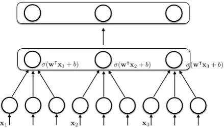
Word Meanings The first type of word (or rather, word meaning) we model picks out a sin-gle object via its visual properties. (At least, this is what we use here; any type of feature could be used.) To model this, we train for each word w from our corpus ofREs a binary logistic regression classifier that takes a representation of a candidate object via visual features (x) and returns a proba-bilitypwfor it being a good fit to the word (where wis the weight vector that is learned andσis the logistic function):
pw(x) =σ(w|x+b) (2)
Formalising the correspondence mentioned above, theintensionof a word can in this approach then be seen as the classifier itself, a function from a representation of an object to a probability:
[[w]]obj =λx.pw(x) (3)
(Where[[w]]denotes the meaning ofw, andxis of the type of feature given by fobj, the function
We train these classifiers using a corpus ofREs (further described in Section 4), coupled with rep-resentations of the scenes in which they were used and an annotation of the referent of that scene. The setting was restricted to reference to single ob-jects. To get positive training examples, we pair each word of a REwith the features of the refer-ent. To get negative training examples, we pair the word with features of (randomly picked) other ob-jects present in the same scene, butnotreferred to by it. This selection of negative examples makes the assumption that the words from the REapply only to the referent. This is wrong as a strict rule, as other objects could have similar visual features as the referent; for this to work, however, this has to be the case only more often than it is not.
The second type of word that we model ex-presses a relation between objects. Its meaning is trained in a similar fashion, except that it is pre-sented a vector of features of a pair of objects, such as their euclidean distance, vertical and hor-izontal differences, and binary features denoting higher than/lower than and left/right relationships.
Application and Composition The model just described gives us a prediction for a pair of word and object (or pair of objects). What we wanted, however, is a distribution over all candidate ob-jects in a given utterance situation, and not only for individual words, but for (incrementally growing) REs. Again as mentioned above, we model two types of application and composition. First, what we call ‘simple references’—which roughly cor-responds to simple NPs—that refer only by men-tioning properties of the referent (e.g. “the red cross on the left”). To get a distribution for a sin-gle word, we apply the word classifier (the inten-sion) to all candidate objects and normalise; this can then be seen as theextensionof the word in a given (here, visual) discourse universe W, which provides the candidate objects (xi is the feature
vector for object i, normalize()vectorized nor-malisation, andI a random variable ranging over the candidates):
[[w]]W obj=
normalize(([[w]]obj(x1), . . . ,[[w]]obj(xk))) =
normalize((pw(x1), . . . , pw(xk))) =P(I|w) (4)
In effect, this combines the individual classifiers into something like a multi-class logistic regres-sion / maximum entropy model—but, nota bene, only for application. The training regime did not
need to make any assumptions about the number of objects present, as it trained classifiers for a 2-class problem (how well does this given object fit to the word?). The multi-class nature is also indi-cated in Figure 1, which shows multiple applica-tions of the logistic regression network for a word, and a normalisation layer on top.
(w|x
1+b) (w|x2+b) (w|x3+b)
[image:3.595.312.532.177.303.2]x1 x2 x3
Figure 1: Representation as network with normalisation layer.
To compose the evidence from individual words w1, . . . , wk into a prediction for a ‘simple’ RE [srw1, . . . , wk](where the bracketing indicates the
structural assumption that the words belong to one, possibly incomplete, ‘simple reference’), we average the contributions of its constituent words. The averaging function avg() over distributions then is the contribution of the construction ‘sim-ple reference (phrase)’,sr, and the meaning of the whole phrase is the application of the meaning of the construction to the meaning of the words:
[[[srw1, . . . , wk]]]W = [[sr]]W[[w1, . . . , wk]]W =
avg([[w1]]W, . . . ,[[w
k]]W) (5)
whereavg()is defined as
avg([[w1]]W,[[w2]]W) =P
avg(I|w1, w2)
withPavg(I=i|w1, w2) =
1
Relational references such as in Exam-ple (1) from the introduction have a more complex structure, being a relation between a (simple) reference to a landmark and a (sim-ple) reference to a target. This structure is indicated abstractly in the following ‘parse’: [rel[srw1, . . . , wk][rr1, . . . , rn][srw10, . . . , w0m]],
where theware the target words,r the relational expression words, andw0the landmark words.
As mentioned above, the relational expression similarly is treated as a classifier (in fact, techni-cally we contract expressions such as “to the left of” into a single token and learn one classifier for it), but expressing a judgement for pairs of objects. It can be applied to a specific scene with a set of candidate objects (and hence, candidate pairs) in a similar way by applying the classifier to all pairs and normalising, resulting in a distribution over pairs:
[[r]]W =P(R1, R2|r) (7) We expect the meaning of the phrase to be a function of the meaning of the constituent parts (the simple references, the relation expression, and the construction), that is:
[[[rel[srw1, . . . , wk][rr][srw01, . . . , w0m]]]] =
[[rel]]([[sr]][[w1. . . wk]],[[r]],[[sr]][[w01. . . w0m]]) (8)
(dropping the indicator for concrete application,
W on [[ ]], for reasons of space and readability).
What is the contribution of the relational con-struction, [[rel]]? Intuitively, what we want to express here is that the belief in an object be-ing the intended referent should combine the ev-idence from the simple reference to the land-mark object (e.g., “the mug” in (1)), from the simple (but presumably deficient) reference to the target object (“the green book on the left”), and that for the relation between them (“next to”). Instead of averaging (that is, combining additively), as for sr, we combine this evidence multiplicatively here: If the target constituent contributes P(It|w1, . . . , wk), the landmark
con-stituent P(Il|w01, . . . , w0m), and the relation
ex-pression P(R1, R2|r), with Il, It, R1 and R2 all
having the same domain, the set of all candidate objects, then the combination is
P(R1|w1, . . . , wk, r, w01, . . . , wm0 ) =
X
R2 X
Il
X
It
P(R1, R2|r)∗P(Il|w01, . . . , w0m)∗
P(It|w1, . . . , wk)∗P(R1|It)∗P(R2|Il) (9)
The last two factors force identity on the elements of the pair and target and landmark, respectively (they are not learnt, but rather set to be 0 unless the values ofRandIare equal), and so effectively reduce the summations so that all pairs need to be evaluated only once. The contribution of the con-struction then is this multiplication of the contri-butions of the parts, together with the factors en-forcing that the pairs being evaluated by the rela-tion expression consist of the objects evaluated by target and landmark expression, respectively.
In the following section, we will explain the data we collected and used to evaluate our model, the evaluation procedure, and the results.
[image:4.595.319.506.296.451.2]4 Experiments
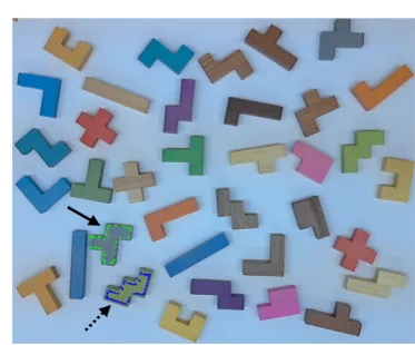
Figure 2: Example episode forphase-2where the target is outlined in green (solid arrow added here for presentation), the landmark outlined in blue (dashed arrow).
Data We evaluated our model using data we col-lected in a Wizard-of-Oz setting (that is, a hu-man/computer interaction setting where parts of the functionality of the computer system were pro-vided by a human experimentor). Participants were seated in front of a table with 36 Pen-tomino puzzle pieces that were randomly placed with some space between them, as shown in Figure 2. Above the table was a camera that recorded a video feed of the objects, processed using OpenCV (Pulli et al., 2012) to segment the objects (see below for details); of those, one (or one pair) was chosen randomly by the experiment software. The video image was presented to the participant on a display placed behind the table, but with the randomly selected piece (or pair of pieces) indicated by an overlay).
(experimentor) had an identical screen depicting the scene but not the selected object. The wiz-ard listened to the participant’sREand clicked on the object she thought was being referred on her screen. If it was the target object, a tone sounded and a new object was randomly chosen. This con-stituted a single episode. If a wrong object was clicked, a different tone sounded, the episode was flagged, and a new episode began. At varied in-tervals, the participant was instructed to “shuffle” the board between episodes by moving around the pieces.
The first half of the allotted time constituted phase-1. After phase-1 was complete, instructions for phase-2 were explained: the screen showed the target and also a landmark object, outlined in blue, near the target (again, see Figure 2). The partici-pant was to refer to the target using the landmark. (In the instructions, the concepts of landmark and target were explained in general terms.) All other instructions remained the same as phase-1. The target’s identifier, which was always known be-forehand, was always recorded. For phase-2, the landmark’s identifier was also recorded.
Nine participants (6 female, 3 male; avg. age of 22) took part in the study; the language of the study was German. Phase-1 for one partici-pant and phase-2 for another participartici-pant were not used due to misunderstanding and a technical diffi-culty. This produced a corpus of 870 non-flagged episodes in total. Even though each episode had 36 objects in the scene, all objects were not always recognised by the computer vision processing. On average, 32 objects were recognized.
To obtain transcriptions, we used Google Web Speech (with a word error rate of 0.65, as deter-mined by comparing to a hand transcribed sample) This resulted in 1587 distinct words, with 15.53 words on average per episode. The objects were not manipulated in any way during an episode, so the episode was guaranteed to remain static during a RE and a single image is sufficient to represent the layout of one episode’s scene. Each scene was processed using computer vision techniques to ob-tain low-level features for each (detected) object in the scene which were used for the word classifiers. We annotated each episode’sREwith a simple tagging scheme that segmented the REinto words that directly referred to the target, words that di-rectly referred to the landmark (or multiple land-marks, in some cases) and the relation words. For
certain word types, additional information about the word was included in the tag if it described colour, shape, or spatial placement (denoted con-tributingREs in the evaluations below). The direc-tionof certain relation words was normalised (e.g.,
left-of should always denote a landmark-target re-lation). This represents a minimal amount of “syn-tactic” information needed for the application of the classifiers and the composition of the phrase meanings. We leave applying a syntactic parser to future work. An example REin the original Ger-man (as recognised by the ASR), English gloss, and tags for each word is given in (2).
(2) a. grauer stein ¨uber dem gr¨unen m unten links b. gray block above the green m bottom left
c. tc ts r l lc ls tf tf
To obtain visual features of each object, we used the same simple computer-vision pipeline of ob-ject segmentation and contour reconstruction as used by Kennington et al. (2015a), providing us with RGB representations for the colour and fea-tures such as skewness, number of edges etc. for the shapes.
Procedure We break down our data as follows: episodes where the target was referred directly via a ‘simple reference’ construction (DD; 410 episodes) and episodes where a target was referred via a landmark relation (RD; 460 episodes). We also test with either knowledge about structure (simple or relational reference) provided (ST) or not (WO, for “words-only”). All results shown are from 10-fold cross validations averaged over 10 runs; where for evaluations labelled RDthe train-ing data always includes all of DDplus 9 folds of RD, testing onRD. The sets address the following questions:
• how well does thesrmodel work on its own with just words? –DD.WO
• how well does the sr model work when it knows aboutREs? –DD.ST
• how well does the sr model work when it knows aboutREs, but not about relations? – RD.ST(sr)
• how well does the model learn relation words after it has learned aboutsr? RD.ST(r) • how well does the rr model work (together
with thesr)?RD.STwithDD.ST(rr)
vocabulary size to 1306. Due to sparsity, for rela-tion words with a token count of less than 4 (found by ranging over values in a held-out set) relational features were piped into an UNK relation, which was used for unseen relations during evaluation (we assume the UNK relation would learn a gen-eral notion of ‘nearness’). For the individual word classifiers, we always paired one negative example with one positive example.
For this evaluation, word classifiers forsrwere given the following features: RGB values, HSV values, x and y coordinates of the centroids, eu-clidean distance of centroid from the center, and number of edges. The relation classifiers received information relating two objects, namely the eu-clidean distance between them, the vertical and horizontal distances, and two binary features that denoted if the landmark was higher than/lower than or left/right of the target.
0 0.1 0.2 0.3 0.4 0.5 0.6 0.7 0.8
DD. WO
DD. ST
RD. ST(sr)
RD. ST(sr+r)
RD. ST(rr)
0.759
0.68
0.608 0.68
0.56
mean reciprocal rank
0 % 10 % 20 % 30 % 40 % 50 % 60 % 70 %
DD. WO
DD. ST
RD. ST(sr)
RD. ST(sr+r)
RD. ST(rr)
65.3 %
55 %
42 %
54 %
40.9 %
[image:6.595.74.296.348.518.2]accuracy
Figure 3:Results of our evaluation.
Metrics for Evaluation To give a picture of the overall performance of the model, we report accu-racy (how often was the argmax the gold target) andmean reciprocal rank(MRR) of the gold tar-get in the distribution over all the objects (like ac-curacy, higherMRRvalues are better; values range between 0 and 1). The use ofMRRis motivated by the assumption that in general, a good rank for the correct object is desirable, even if it doesn’t reach the first position, as when integrated in a dialogue system this information might still be useful to for-mulate clarification questions.
Results Figure 3 shows the results. (Random baseline of 1/32 or 3% not shown in plot.)DD.WO shows how well the srmodel performs using the whole utterances and not just the REs. (Note that
all evaluations are on noisy ASR transcriptions.) DD.ST adds structure by only considering words that are part of the actual RE, improving the re-sults further. The remaining sets evaluate the con-tributions of the rr model. RD.ST (sr) does this indirectly, by including the target and landmark simple references, but not the model for the rela-tions; the task here is to resolve target and land-mark SRs as they are. This provides the baseline for the next two evaluations, which include the re-lation model. In RD.ST (sr+r), the model learns SRs fromDDdata and only relations fromRD. The performance is substantially better than the base-line without the relation model. Performance is best finally for RD.ST (rr), where the landmark and target SRs in the training portion of RD also contribute to the word models.
Themean reciprocal rankscores follow a sim-ilar pattern and show that even though the target object was not the argmax of the distribution, on average it was high in the distribution. For all eval-uations, the average standard deviation across the 10 runs was very small (0.01), meaning the model was fairly stable, despite the possibility of one run having randomly chosen more discriminating neg-ative examples. Our conclusion from these exper-iments is that despite the small amount of training data and noise fromASRas well as the scene, the model is robust and yields respectable results.
0 2 4 6 8 10 12 14
[image:6.595.314.514.486.623.2]5 0 5 10 15 20 25
Figure 5: Incremental results: average rank improves over time
Incremental Results Figure 5 shows how our rr model processes incrementally, by giving the
100 200 300 400 500 600 100
200 300 400
0.1 0.2 0.3 0.4 0.5 0.6 0.7 0.8 0.9
0 50 100 150 200 250 0.0
0.2 0.4 0.6 0.8 1.0
100 200 300 400 500 600 100
200 300 400
[image:7.595.94.497.70.162.2]0.0 0.1 0.2 0.3 0.4 0.5 0.6 0.7 0.8 0.9
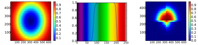
Figure 4: Each plot represents how well selected words fit assumptions about their lexical semantics: the leftmost plotecke (corner) yields higher probabilities as objects are closer to the corner; the middle plotgr¨un(green) yields higher probabilities when the colour spectrum values are nearer to green; the rightmost plot¨uber(above) yields higher probabilities when targets are nearer to a landmark set in the middle.
Figure is as expected. There is a slight increase between 6-7, though very small (a difference of 0.09). Overall, these results seem to show that our model indeed worksintersectivelyand “zooms in” on the intended referent.
4.1 Further Analysis
Analysis of Selected Words We analysed sev-eral individual word classifiers to determine how well their predictions match assumptions about their lexical semantics. For example, for the spa-tial wordEcke(corner), we would expect its clas-sifier to return high probabilities if features related to an object’s position (e.g., x and y coordinates, distance from the center) are near corners of the scene. The leftmost plot in Figure 4 shows that this is indeed the case; by holding all non-position features constant and ranging over all points on the screen, we can see that the classifier gives high probabilities around the edges, particularly in the four corners, and very low probabilities in the mid-dle region. Similarly for the colour word gr¨un, the centre plot in Figure 4 (overlaid with a colour spectrum) shows high probabilities are given when presented with the colour green, as expected. Sim-ilarly, for the relational word ¨uber (above), by treating the center point as the landmark and rang-ing over all other points on the plot for the target, the ¨uber classifier gives high probabilities when directly above the center point, with linear nega-tive growth as the distance from the landmark in-creases.
Note that we selected the type of feature to vary here for presentation; all classifiers get the full fea-ture set and learn automatically to “ignore” the ir-relevant features (e.g., that for gr¨un does not re-spond to variations in positional features). They do this wuite well, but we noticed some ‘blurring’, due to not all combinations of colours and shape being represented in the objects in the training set.
Analysis of Incremental Processing Figure 6 finally shows the interpretation of the RE in Ex-ample (2) in the scene from Figure 2. The top row depicts the distribution over objects (true tar-get shown in red) after the relation word unten
(bottom) is uttered; the second row that for land-mark objects, after the landland-mark description be-gins (dem gr¨unen m/the green m). The third row (target objects), ceases to change after the rela-tional word is uttered, but continues again as ad-ditional target words are uttered (unten links/ bot-tom left). While the true target is ranked highly already on the basis of the target SR alone, it is only when the relational information is added (top row) that it becomes argmax.
Discussion We did not explore how well our model could handle generalised quantifiers, such asall(e.g.,all the red objects) or a specific num-ber of objects (e.g.,the two green Ts). We specu-late that one could see as the contribution of words such asallortwoa change to how the distribution is evaluated (“return thentop candidates”). Our model also doesn’t yet directly handle more de-scriptiveREs likethe cross in the top-right corner on the left, asleft is learned as a global term, or negation (the cross that’s not red). We leave ex-ploring such constructions to future work.
5 Related Work
grauer stein über dem grünen m unten links
Figure 6:A depiction of the model working incrementally for theREin Example (2): the distribution over objects for relation is row 1, landmark is row 2, target is row 3.
formal semantics for similarly descriptive terms, where parts of the semantics are modelled by a perceptual classifier. These approaches had lim-ited lexicons (where we attempt to model all words in our corpus), and do not process incrementally, which we do here.
Recent efforts in multimodal distributional se-mantics have also looked at modelling word mean-ing based on visual context. Originally, vector space distributional semantics focused words in the context of other words (Turney and Pantel, 2010); recent multimodal approaches also con-sider low-level features from images. Bruni et al. (2012) and Bruni et al. (2014) for example model word meaning by word and visual con-text; each modality is represented by a vector, fused by concatenation. Socher et al. (2014) and Kiros et al. (2014) present approaches where words/phrases and images are mapped into the same high-dimensional space. While these ap-proaches similarly provide a link between words and images, they are typically tailored towards a different setting (the words being descriptions of the whole image, and not utterance intended to perform a function within a visual situation). We leave more detailed exploration of similarities and differences to future work and only note for now that our approach, relying on much simpler classifiers (log-linear, basically), works with much smaller data sets and additionally seem to pro-vide an easier interface to more traditional ways of composition (see Section 3 above).
The issue of semantic compositionality is also actively discussed in the distributional semantics literature (see, e.g., (Mitchell and Lapata, 2010; Erk, 2013; Lewis and Steedman, 2013; Paperno
et al., 2014)), investigating how to combine vec-tors. This could be seen as composition on the level of intensions (if one sees distributional rep-resentations as intensions, as is variously hinted at, e.g. Erk (2013)). In our approach, composition is done on the extensional level (by interpolating distributions over candidate objects).
We do not see our approach as being in op-position to these attempts. Rather, we envision a system of semantics that combines traditional symbolic expressions (on which inferences can be modelled via syntactic calculi) with distributed representations (which model conceptual knowl-edge / semantic networks, as well as encyclopedic knowledge) and with our action-based (namely, identification in the environment via perceptual information) semantics. This line of approach is connected to a number of recent works (e.g., (Erk, 2013; Lewis and Steedman, 2013; Larsson, 2013)); for now, exploring its ramifications is left for future work.
6 Conclusion
repre-sentation.
Our next steps with this model is to handle com-positional structures without relying on our closed tag set (e.g., using a syntactic parser). We also plan to test our model in a natural, interactive dia-logue system.
Acknowledgements We want to thank the anonymous reviewers for their comments. We also want to thank Spy-ros Kousidis for helping with data collection, Livia Dia for help with the computer vision processing, and Julian Hough for fruitful discussions on semantics, though we can’t blame them for any problems of the work that may remain. This re-search/work was supported by the Cluster of Excellence Cog-nitive Interaction Technology ’CITEC’ (EXC 277) at Biele-feld University, which is funded by the German Research Foundation (DFG).
References
Elia Bruni, Gemma Boleda, Marco Baroni, and Nam-Khanh Tran. 2012. Distributional semantics in tech-nicolor. InProceedings of the 50th Annual Meet-ing of the Association for Computational LMeet-inguis- Linguis-tics, volume 1, pages 136–145.
Elia Bruni, Nam Khanh Tran, and Marco Baroni. 2014. Multimodal distributional semantics. Journal of Ar-tificial Intelligence Research, 49:1–47.
Herbert H Clark. 1996. Using Language, volume 23. Cambridge University Press.
Nikos Engonopoulos, Martin Villalba, Ivan Titov, and Alexander Koller. 2013. Predicting the resolu-tion of referring expressions from user behavior. In
Proceedings of EMLNP, pages 1354–1359, Seattle,
Washington, USA. Association for Computational Linguistics.
Katrin Erk. 2013. Towards a semantics for distri-butional representations. InProceedings of IWCS, pages 1–11, Potsdam, Germany.
Charles J Fillmore. 1975. Pragmatics and the descrip-tion of discourse. Radical pragmatics, pages 143– 166.
Kotaro Funakoshi, Mikio Nakano, Takenobu Toku-naga, and Ryu Iida. 2012. A Unified Probabilis-tic Approach to Referring Expressions. In
Proceed-ings of SIGDial, pages 237–246, Seoul, South
Ko-rea, July. Association for Computational Linguistics. L T F Gamut. 1991. Logic, Language and Meaning:
Intensional Logic and Logical Grammar, volume 2.
Chicago University Press, Chicago.
Peter Gorniak and Deb Roy. 2004. Grounded semantic composition for visual scenes. Journal of Artificial Intelligence Research, 21:429–470.
Stevan Harnad. 1990. The Symbol Grounding
Prob-lem.Physica D, 42:335–346.
John Kelleher, Fintan Costello, and Jofsef Van Gen-abith. 2005. Dynamically structuring, updating and interrelating representations of visual and lin-guistic discourse context. Artificial Intelligence, 167(1–2):62–102.
Casey Kennington, Spyros Kousidis, and David Schlangen. 2013. Interpreting Situated Dialogue Utterances: an Update Model that Uses Speech, Gaze, and Gesture Information. InProceedings of SIGdial.
Casey Kennington, Spyros Kousidis, and David Schlangen. 2014. Situated Incremental Natu-ral Language Understanding using a Multimodal, Linguistically-driven Update Model. In Proceed-ings of CoLing.
Casey Kennington, Livia Dia, and David Schlangen. 2015a. A Discriminative Model for Perceptually-Grounded Incremental Reference Resolution. In
Proceedings of IWCS. Association for
Computa-tional Linguistics.
Casey Kennington, Ryu Iida, Takenobu Tokunaga, and David Schlangen. 2015b. Incrementally Track-ing Reference in Human/Human Dialogue UsTrack-ing Linguistic and Extra-Linguistic Information. In
NAACL, Denver, U.S.A. Association for
Computa-tional Linguistics.
Ryan Kiros, Ruslan Salakhutdinov, and Richard S Zemel. 2014. Unifying Visual-Semantic Embed-dings with Multimodal Neural Language Models.
InProceedings of NIPS 2014 Deep Learning
Work-shop, pages 1–13.
Staffan Larsson. 2013. Formal semantics for percep-tual classification. Journal of Logic and Computa-tion.
Mike Lewis and Mark Steedman. 2013. Combined Distributional and Logical Semantics. Transactions of the ACL, 1:179–192.
Edward Loper and Steven Bird. 2002. NLTK: The nat-ural language toolkit. InProceedings of the ACL-02 Workshop on Effective tools and methodologies for teaching natural language processing and computa-tional linguistics-Volume 1, pages 63–70. Associa-tion for ComputaAssocia-tional Linguistics.
Cynthia Matuszek, Liefeng Bo, Luke Zettlemoyer, and Dieter Fox. 2014. Learning from Unscripted Deic-tic Gesture and Language for Human-Robot Interac-tions. InAAAI. AAAI Press.
Richard Montague. 1973. The Proper Treatment of Quantifikation in Ordinary English. In J Hintikka, J Moravcsik, and P Suppes, editors,Approaches to Natural Language: Proceedings of the 1970
Stan-ford Workshop on Grammar and Semantics, pages
221–242, Dordrecht. Reidel.
Denis Paperno, Nghia The Pham, and Marco Baroni. 2014. A practical and linguistically-motivated ap-proach to compositional distributional semantics. In
Proceedings of ACL, pages 90–99.
Barbara H Partee, Alice ter Meuelen, and Robert E Wall. 1993. Mathematical Methods in Linguistics. Kluwer Academic Publishers, Dordrecht.
Kari Pulli, Anatoly Baksheev, Kirill Kornyakov, and Victor Eruhimov. 2012. Real-time computer vi-sion with OpenCV. Communications of the ACM, 55(6):61–69.
Richard Socher, Andrej Karpathy, Quoc V Le, Christo-pher D Manning, and Andrew Y Ng. 2014. Grounded Compositional Semantics for Finding and Describing Images with Sentences. Transactions of the Association for Computational Linguistics (TACL), 2:207–218.
Luc Steels and Tony Belpaeme. 2005. Coordinating perceptually grounded categories through language: a case study for colour. The Behavioral and brain sciences, 28(4):469–489; discussion 489–529. Peter D Turney and Patrick Pantel. 2010. From