Performance Estimation of HEVC/h 265 Decoder in a Co Design Flow with SADF FSM Graphs

ISSN Online: 1913-3723 ISSN Print: 1913-3715

DOI: 10.4236/ijcns.2017.1011016 Nov. 14, 2017 261 Int. J. Communications, Network and System Sciences

Performance Estimation of HEVC/h.265

Decoder in a Co-Design Flow with

SADF-FSM Graphs

Habib Smei

, Abderrazak Jemai

, Kamel Smiri

1_{Laboratory LIP2, Faculty of Sciences of Tunis, University of Tunis El Manar, Tunis, Tunisie}

2_{General Directorate of Technological Studies, Higher Institute of Technological Studies of Rades, Ben Arous, Tunisia} 3_{University of Carthage, National Institute of Applied Science and Technology, Tunis, Tunisie}

4_{University of Manouba, Higher Institute of Multimedia Arts of Manouba, Manouba, Tunisie}

Abstract

Multiprocessor System on Chip (MPSoC) technology presents an interesting solution to reduce the computational time of complex applications such as multimedia applications. Implementing the new High Efficiency Video Cod-ing (HEVC/h.265) codec on the MPSoC architecture becomes an interestCod-ing research point that can reduce its algorithmic complexity and resolve the real time constraints. The implementation consists of a set of steps that compose the Co-design flow of an embedded system design process. One of the first anf key steps of a Co-design flow is the modeling phase which allows designers to make best architectural choices in order to meet user requirements and plat-form constraints. Multimedia applications such as HEVC decoder are com-plex applications that demand increasing degrees of agility and flexibility. These applications are usually modeling by dataflow techniques. Several ex-tensions with several schedules techniques of dataflow model of computation have been proposed to support dynamic behavior changes while preserving static analyzability. In this paper, the HEVC/h.265 video decoder is modeled with SADF based FSM in order to solve problems of placing and scheduling this application on an embedded architecture. In the modeling step, a high-level performance analysis is performed to find an optimal balance be-tween the decoding efficiency and the implementation cost, thereby reducing the complexity of the system. The case study in this case works with the HEVC/h.265 decoder that runs on the Xilinx Zedboard platform, which offers a real environment of experimentation.

Keywords

HEVC, h.265, Performance Estimation, SDF, SADF, SADF-FSM, Embedded How to cite this paper: Smei, H., Jemai, A.

and Smiri, K. (2017) Performance Estima-tion of HEVC/h.265 Decoder in a Co-Design Flow with SADF-FSM Graphs. Int. J. Com-munications, Network and System Sciences, 10, 261-281.

https://doi.org/10.4236/ijcns.2017.1011016

Received: August 7, 2017 Accepted: November 11, 2017 Published: November 14, 2017

Copyright © 2017 by authors and Scientific Research Publishing Inc. This work is licensed under the Creative Commons Attribution International License (CC BY 4.0).

http://creativecommons.org/licenses/by/4.0/

DOI: 10.4236/ijcns.2017.1011016 262 Int. J. Communications, Network and System Sciences Systems

1. Introduction

The evolution of digital video industry is being driven by continuous improve-ments in processing performance, availability of higher-capacity storage and transmission mechanisms. The increasing complexity of embedded applications deployed on Multiprocessor Systems-on-Chip (MPSoC) ranging from multime-dia applications and telecommunications to aerospace applications has raised problems related to performance estimation and evaluation. The designer must have a view of the execution time of the various functions of the system to be de-signed, the memory size, the energy consumed, the silicon space of the hardware components and other necessary parameters to take decisions for architectural solutions. Performance evaluation in embedded systems can be carried out by different methods; either by measurement, by simulation or by analytical me-thods. Analytical methods are based on mathematical models to represent the application on one hand and the hardware platform on the other hand and then to apply performance estimation algorithms to analyze them.

Although these analytical approaches are less precise than approaches based on measurements and simulation, they are characterized by their speed and high level of abstraction allowing the designer to make quick decisions for the archi-tectural choices of the system to be designed. Analytical methods represent the system to be conceived as a set of competing processes or actors linked through communication channels and called Model of computation. A Model of Com-putation (MoC) determines the rules that are used for comCom-putation inside processes and communication between processes. Models of computation allow abstracting the implementation of computation and communication in the sys-tem. Once system functionality is expressed using a MoC, this model can be subjected to transformations and analysis to reach an efficient implementation. There are many MoCs in the literature [1][2][3]. One of the most MoCs used to model streaming applications is Synchronous Data Flow (SDF) [4] [5]. Our work is concerned by the use of a variant of SDF graphs called SADF to estimate analytically the maximal achievable throughput of a multitask application under design. SDF Graphs (called also multi-rate regular dataflow graphs), initially proposed by Lee [6], are directed graphs where edges represent one-to-one data channels and whose vertices represent actors or tasks that operate on that data. As soon as all the input data have arrived, these actors begin their execution, af-ter which they produce their output data. As long as such a data flow model is analyzable, performance guarantees can be obtained at design time.

2. Related Works

DOI: 10.4236/ijcns.2017.1011016 263 Int. J. Communications, Network and System Sciences Stuijk [7] is the first person who proposed an SDF graph to map a multimedia application on NoC-MPSoC platforms in order to minimize the resource usage. The flow begins with an application-aware SDF that is gradually transformed to handle resource sharing over a multi-tile architecture. In [8], authors use timed SDF graph to model NoC architectures with predefined guaranteed of band-width and a maximum latency. Several predictable arbitration mechanisms of MPSOC and NoC have been used, such as Round robin, TDMA, and Static sharing.In [9], authors studied the use of SDF in performance estimation after task migration from software to hardware. In [10], authors proposed an ap-proach that uses Resource Manager (RM) actor to analyze applications that are modeled with SDF graphs. RM is a task responsible for resources access (critical or not). The designer reserves for the RM a whole execution node (CPU, mem-ory, bus...) which increases the cost of the total MPSoC system. In [11], Wiggers

et al. proposed a solution that exploits the SDF graphs to compare the through-put obtained with the target throughthrough-put of the application. SDF is used for the modeling sharing multi-port memory tiles in order to generate the best alloca-tion. In [12], authors use SDFs to estimate the worst-case performance of a sys-tem before implementation. They developed a generic communication assistant module for multi-processors and multi-applications systems. In [13] [14], au-thors use FSM-SADF in order to model dynamic applications with multiple ex-ecution scenarios. Each scenario (behavior) is modeled by an SDF, and the FSM represents the possible orders in which active scenarios occur. Astochastic ver-sion of the SADF model is studied in [15]. In addition, in [16] homogeneous SDF graphs are considered (graphs in which all consumption and production rates are equal to one) to use SDF behavior. Only the execution times of affixed collection of actors can vary with scenarios. The approach presented in [17] is the most related to this work. It uses essentially the same model of computation, Scenario-Aware Dataflow Graphs (SADF). It introduces an analysis technique that works by building up a global state-space representation of the detailed be-havior of the graph across sequences of scenarios. Transitions are at the level of individual firings of actors. This tends to lead to very large state spaces and trac-tability issues with larger models. [18] deals with scenarios of SDF behavior, but in their case only homogeneous SDF graphs are considered (graphs in which all consumption and production rates are equal to one), and only the execution times of affixed collection of actors can vary with scenarios. In [19], authors tried to find linear upper bounds on transient behavior of an SDF; this allows the behavior of an SADF to be analyzed.

3. Background

DOI: 10.4236/ijcns.2017.1011016 264 Int. J. Communications, Network and System Sciences necessary information for co-design steps.

Specification is usually represented as a software application coded with a high level language such as C/C++, Matlab, Sytemc. This specification is run on a host machine in order to test its functionalities and further understand the specificities of the whole system. Once this specification is tested, a profiling step [21][22] is usually performed to define a profile of each entity of the system and establish a call graph function as well as other information such as execution time, size and type of data Exchanged. All this information is a parameter whose designers use to define architectural choices either in the modeling phase and partitioning phase of the Co-design flow. Once the modeling is done, a verifica-tion of the established model is required. Several methods, languages and tools are available to designers to do this verification. The choice of tools and ap-proaches depends essentially on the nature of the application to be modeled (for example, data flow oriented or control flow oriented), but also depends on the experience of the design team and the availability of tools grasped.

Usually the verification step is performed by simulation, hardware emulation or by formal methods (e.g. Model Checking, Theorem Proving...). But when ap-plications become increasingly complex (e.g. Multimedia apap-plications) and ar-chitectures are increasingly powerful (e.g. MPSOCs), the use of these traditional verification methods on complex embedded systems appears increasingly ineffi-cient. In fact, the use of traditional methods of verification with these new sys-tems consumes either an intolerable processing time (e.g. logic simulation), or an exaggerated memory size (e.g. Model Checking). For this purpose, designers have recourse to new modeling and verification methods, namely Model of Computation (MOC).

3.1. Data Flow Model of Computation

DOI: 10.4236/ijcns.2017.1011016 265 Int. J. Communications, Network and System Sciences by specifying the data production/consumption rate as an integer value for each actors interconnection. Such information allows certifying the application to be deadlock free and to compute a statically schedule and computer memory re-quirements. In order to allow the expressiveness of the rather restrictive SDF model, several models were issued. The Boolean Data Flow Model (BDF) [24] aims at introducing switching and selection instructions into the SDF model. Boolean data flow (BDF), for instance, extends the SDF model of computation with two special actors called switch and select. The first one reads one input to-ken and forward it to one of two possible outputs. The output to select is speci-fied by a second Boolean input port. In the same way the select actor reads a to-ken from one of two possible inputs and forwards it to a single output port. Al-ready these simple extensions together with unbounded FIFOs are sufficient to generate a Turing complete model of computation. Integer-controlled data flow (IDF) [25] is an extension of BDF in that the switch and select actors can have more outputs or inputs, respectively. Whereas this helps to simplify the applica-tion models, it does not offer further expressiveness, as BDF is already Turing complete. Cyclo-dynamic data flow (CDDF) [26] aims to enhance the analysis capabilities of dynamic data flow descriptions. Its major idea is to provide more context information about the problem to analysis tools than this is done by BDF. For this reason, an actor executes a sequence of phases whose length de-pends on a control token. The latter can be transported on any edge, but must be part of a finite set. Each phase can have its own consumption and production behaviour, which can even depend on control tokens. Several restrictions take care that the scheduler can derive more context information, as this would be the case for BDF graphs. For instance, a CDDF actor is not allowed to have a hidden internal state.

3.2. Synchronous Data Flow

Synchronous dataflow (SDF) [27] [28] network is composed of actors that are connected by FIFO channels. When an actor fires, it consumes tokens from in-put channels and produces tokens on outin-put channels. Firings of an SDF actor create a process. The actor’s firing rule specifies how many tokens are consumed on each input and how many will be produced on each output. In SDF, the number of tokens consumed on each input in every firing is constant, ie the fir-ing rule remains the same.

The constant number of chips consumed and produced makes possible to make very efficient statics schedules.

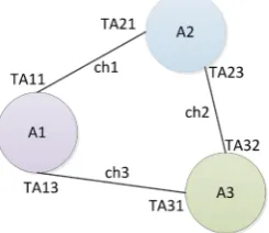
Figure 1 presents an SDF graph with three actors. Consumption and produc-tion rates of tokens are labeled on each channel. For example, the consumpproduc-tion and production rates in channel ch3 are respectively TA13 and TA31.

DOI: 10.4236/ijcns.2017.1011016 266 Int. J. Communications, Network and System Sciences Figure 1. Example of a SDF graph.

iteration. To accomplish the first step, we must solve the set of balance equa-tions. Balance equations state that production and consumption of tokens must be equal on all channels. The balance equations for the SDF graph the Figure 1 are shown below.

1 11 2 21

1 13 3 31

3 32 2 23

FA TA FA TA

FA TA FA TA

FA TA FA TA

× = ×

× = ×

× = ×

FA1, FA3, FA2 are integers showing how many times actors A1, A2 and A3 fire in a single iteration. They form a firing or repetition vector. The least posi-tive integer solution is taken. For example if TA11 = 2, TA13 = 2, TA31 = 3,

TA32 = 3, TA21 = 6 and TA23 = 6 then FA1 = 3, FA3 = 2 and FA2 = 1. We must resolve this equation: FA1 2× =FA2 6× and FA1 2× =FA3 3× and

3 3 2 6

FA × =FA × . We have as solution FA1 = 3, FA3 = 2 and FA2 = 1

If we have as solution zero (the only solution), then the SDF graph is said to be inconsistent. This means that production and consumption of tokens cannot be balanced on all channels. As a result, the executions of an inconsistent SDF graph.

DOI: 10.4236/ijcns.2017.1011016 267 Int. J. Communications, Network and System Sciences of separate behaviors, called scenarios or modes. Each scenario is static and pre-dictable in performance and resource utilization. It can therefore be treated by traditional methods. However, some other difficulties need to be addressed such as predicting scenarios and handling transitions between them.

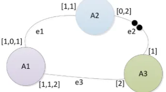
In this work, we use the Scenario-Aware Dataflow (SADF) [14] generalization of CSDF (Figure 2, Figure 3), which is based on scenarios to model the embed-ded software and the target hardware platform. SADF characterizes each scena-rio or individual mode by a specific SDF graph that models tasks with constant worst-case execution times. A finite state machine (FSM) is used for the Transi-tions between scenarios.

The HEVC Decoder is a dynamic application with several execution scenarios. Therefore, it cannot be modeled by SDF. The FSM-based-SADF extension is the suitable to model the application for a specific class of bitstream. Indeed, for a given class (a fixed frames resolution), it is possible to have four possible confi-gurations (AI, RA, LP, LB) and several execution scenarios. The management of the various scenarios is carried out using a finite state machine (FSM).

4. Our Approach of MPSoC Co-Design Oriented Performance

Evaluation

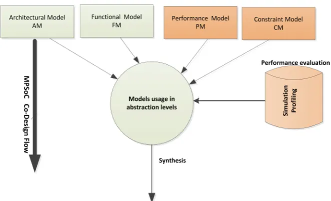
Our goal for using SDF in our Co-design flow is the performance estimation. It enables us to carry out measurements relating to execution time, energy con-sumption, memory space of the various functions and other necessary informa-tion for Co-design steps. Figure 4 presents our approach of MPSoC Co-design oriented performance evaluation. This approach is structured around four mod-els:Functional Model (MF) of the application that describes the application be-havior, Architecture Model AM which describes the target platform in number of processors, cache memory, communication system Bus/NoC…, Constraint Model (CM)in which constraints are specified and Performance Model (PM) that is used to provide performance metrics such as execution time and throughput. The two new models that we introduce in this approach are the PM and the CM models. These are two key models that guide the designer in the architectural choices during the Co-design process of the MPSoC system. The Constraint Model (CM) describes the functional constraints of the application and non-functional constraints of the target platform. The Performance Model

DOI: 10.4236/ijcns.2017.1011016 268 Int. J. Communications, Network and System Sciences Figure 3. Example of a SADF graph.

Figure 4. Approach of MPSoC Co-design oriented Performance estimation.

PM describes a performance evaluation of the system in every abstraction level. Every refinement of system is followed by a refinement of the correspondent PM model. The PM is enriched by results gotten by techniques and tools of perfor-mance evaluation. The PM is more precise to the lowest abstraction levels. It takes into account the task parallel model, Software/Hardware partition, Oper-ating System Real Time(RTOS), hardware architecture(type and number of the processors, size of RAM and size of cache memory) and communication system (Bus, NoC).

DOI: 10.4236/ijcns.2017.1011016 269 Int. J. Communications, Network and System Sciences should be explored at this abstraction level otherwise additional details will be added to these models.

Starting from a pure functional model of the application, the following details are gradually added:the number of processing elements, the HW/SW partition-ing, the hardware topologies, scheduling techniques used by the embedded OSs, Communication network architecture, HAL, etc. Both analytic and simulation techniques are used during the estimation.

5. Case Study: HEVC/h.265 Decoder

The HEVC standard [29][30] is based on hybrid video coding based blocks. It implements the concept of block partitioning, which divides the image into blocks. Each block is predicted using either intra-frame or inter picture predic-tion. Intra-frame exploits spatial redundancy between the blocks within an im-age. Inter-picture uses the temporal redundancy between pictures. The predic-tion error is made by the difference between the original image and the pre-dicted image in the case of both intra- and inter-picture prediction. The result-ing prediction error is transmitted to the transform codresult-ing means followed by quantization and entropy coding. In the previous version of the standard HEVC (AVC, h.264) [31], the division of a frame is done according to 16 × 16 ma-cro-blocks. In HEVC, h.265, a frame can be divided into “coding tree blocks” (CTBs). Depending by an encoding setting, the size of the CTB can be of 64 × 64, 32 × 32 or 16 × 16. Indeed, several studies have shown that bigger CTBs pro-vide higher efficiency (but also higher encoding time). Each CTB can be split recursively, in a quad-tree structure, in 32 × 32, 16 × 16 down to 8 × 8 sub-regions, called coding units (CUs).

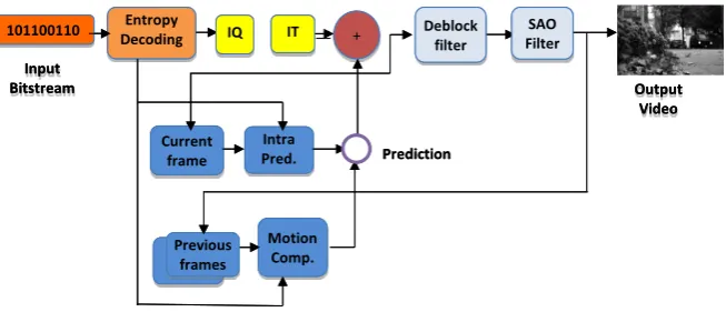
In HEVC, CUs are the basic unit of prediction. Usually smaller CUs are used around detailed areas (edges and so on), while bigger CUs are used to predict flat areas. Each CU can be recursively divided into Transform Units (TUs) or Prediction Units (PUs) with the same quad-tree approach used in CTBs. Unlike AVC that used mainly a 4 × 4 transform and occasionally an 8 × 8 transform, HEVC has several transform sizes: 32 × 32, 16 × 16, 8 × 8 and 4 × 4. The trans-forms are based on DCT (Discrete Cosine Transform) except for intra 4 × 4, when transform is based on DST instead (Discrete Sine Transform) because sev-eral tests have evidenced a small improvement in compression. The HEVC de-coder takes as an input a compressed file called bit-stream from which it extracts and decodes all the syntax elements, and then constructs each frame of the orig-inal video sequence. Figure 5 illustrates a common architecture of the HEVC decoder.

DOI: 10.4236/ijcns.2017.1011016 270 Int. J. Communications, Network and System Sciences Figure 5. Block diagram of HEVC Decoder.

Quantized and transformed coefficients are handled, respectively, by the in-verse quantization (IQ module in Figure 5) and the inverse transform (IT mod-ule, in Figure 5). The prediction process can be either intra-prediction or mo-tion compensamo-tion (inter-predicmo-tion). The intra predicmo-tion block operates when the frame is an I frame. The inter prediction block operates when the frame is a P or B frame. The next step, before filtering is the storage of the reconstructed samples, the residue added to the predicted samples. This latter, will be used as references by the intra-frame or the inter-frame prediction modules.

The third step is the Loop filter composed by two filters blocks. The first is Deblocking Filter (DF) applied at the boundaries of the reconstructed blocks. It reduces the mean sample distortion of the decoded frame compared to the orig-inal one. The second is a new filter introducing with HEVC called Sample Adap-tive Offset (SAO). It transmits offset values that can either resemble to the inten-sity band of pixel values (band offset) or the difference compared to neighboring pixels (edge offset).

6. FSM-SADF Model of HEVC/265 Decoder

To model an application with an SDF graph, the designer must have at his dis-posal information that concern the application, its functions (actors), the ex-changed data (tokens) and their sizes, the size of the data used in each function and constraints to which the application is subject. This information can be ex-tracted by performing a fine profiling step of the application. We have thus per-formed a profiling step that combines manual profiling with the use of available profiling tools such as Valgrind [32], Gpr of [33], mempr of [34]. Sequences used in this work are extracted from reference sequences and configurations proposed by the JCT-VC [35]. The sequences are divided into 6 groups (Classes). Group A corresponds to sequences with a resolution of 2560 × 1600 pixels, group B contains sequences with a resolution of1920 × 1080, group C consists of sequences with a resolution of 832 × 480 pixels, sequences of groups D have a resolution of 416 × 240 pixels and Group E consists of sequences with a

Diagram Block of HEVC decoder

Output Video Entropy Decoding + Current frame Intra Pred. Motion Comp. Previous frames 101100110 Input Bitstream IT IQ Prediction SAO Filter Deblock filter

Diagram Block of HEVC decoder

DOI: 10.4236/ijcns.2017.1011016 271 Int. J. Communications, Network and System Sciences resolution of 1280 × 720. The last group, F consists of sequences with a resolu-tion of 1024 × 768.

Our work is based on the HEVC HM Test Model [36]. This is an open source project under BSD license. It is intended for the implementation of an efficient HEVC C++ decoder. The version used in this work has been downloaded from [36] and it is compliant with the HEVC standard. Our profiling strategies are described in previous work [22][30].

6.1. Actors Identification and Dependencies

To determine actors of the system and the relations between them, we check the behavior of the decoder described above by carrying out a parametric analysis of the application.

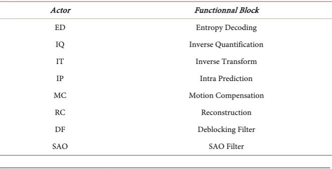
According to the profile stage, we identify eight actors as presented in Table 1. Each actor represents a set of C++ classes in the HM test Model application.

6.2. Number and Size of Data Exchanged (Tokens Exchanged)

It is necessary to observe the data exchanged in the different configurations and to choose the largest number and the largest size. We must therefore define this information for the different classes (A, B,∙∙∙, F). We will take as an example the class C that corresponds to the 832 × 480 resolution which corresponds to 399,360 pixels. So the size will be 399,360 × 4 = 1,597,440 bytes. According to the rule of the worst case, the size of CTU that will be chosen is 16 × 16 (256). So the maximum number of CTUs (tokens) exchanged will be: (832 × 480)/256 or 399360/256 = 1560 CTU (case of class C).

The data exchanged between the different actors of the HEVC CODEC are: - Residual CTUs that are processed by IQ, IT actors. The maximum size of a

CTU is 64 × 64 or 4096 pixels or 16,384 bytes.

- Intra-prediction data (from the ED block to the Intra-prediction), it can be at most a CTU that is: 16,384 bytes.

Table 1. Actors of HEVC Decoder.

Actor Functionnal Block

ED Entropy Decoding

IQ Inverse Quantification

IT Inverse Transform

IP Intra Prediction

MC Motion Compensation

RC Reconstruction

DF Deblocking Filter

DOI: 10.4236/ijcns.2017.1011016 272 Int. J. Communications, Network and System Sciences - Inter-prediction data (from the ED block to the Inter-prediction block or MC

block) composed of the motion vectors. Each motion vector is encoded with 12 bytes (array of 3 integers). Indeed, the motion vector is composed of 3 parameters, the origin, the angle and its length. Each one coded by 1 byte.

- An unfiltered image (from the RC block to the Loop Filter block), 399,360 pixels* 4 bytes or 1,597,440 bytes (size of a frame for class C).

- A full filtered image (from the Loop Filter block to the prediction blocks, IP and MC), 399,360 bytes or 1,597,440 bytes (size of a frame for class C). - Useful data for the Loop Filter block (from the ED block to the SAO filter). It

can be maximum 5 bytes.

6.3. Number of Motion Vectors

The number of motion vectors is always less than or equal to the number of CTUs (it will be equal if all the CTUs that exist in the current image also exist in the reference image even if they change positions) because a vector of Movement carries information about a CTU that has a copy in the reference image. To do this, we can fix the Maximum number of motion vectors in a frame at 1560 (the number of CTUs in a class C frame).

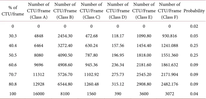
This will pose a modeling problem since it is difficult to create a scenario for each case (i.e. 1561 cases for class C, for example). According to a work in [37], the number of blocks that have motion vectors in a frame obeys a probabilistic law. We rely on the values proposed in the following table (Table 2) and the curve of Figure 6.

Actually, and observing this probability curve, we can note that this charts has a spike between values 30.3% and 60.6%. So it is possible to limit the choice of the values representative of the possible cases of the motion vectors, which are very numerous as it is already mentioned. It can be limited to values in this in-terval and moreover one will try to distribute the chosen values along the chosen portion of the interval to be near to the real values whatever the case (the real value falls always close to one of the approximate values).

6.4. Scenarios Determination

An application that changes its mode of operation according to its input is a dy-namic application. Therefore, it must be modeled with dydy-namic modeling. Each use case will have its own parameters (execution time, memory size, number of tokens exchanged....) and therefore corresponds to an execution scenario. The HEVC decoder is an example of dynamic applications with multiple execution scenarios. Indeed, for a given class (A, B, C,∙∙∙, F), the operation mode of the de-coder depends on three parameters:

- The type of frame to be decoded (I, P or B).

DOI: 10.4236/ijcns.2017.1011016 273 Int. J. Communications, Network and System Sciences Figure 6. Probability of the numbers of motion vectors.

Table 2. Percentage and number of CTU/frame with motion vectors

% of CTU/frame

Number of CTU/Frame

(Class A)

Number of CTU/Frame (Class B)

Number of CTU/Frame (Class C)

Number of CTU/Frame (Class D)

Number of CTU/Frame (Class E)

Number of CTU/Frame

(Class F) Probability

0 0 0 0 0 0 0 0.02

30.3 4848 2454.30 472.68 118.17 1090.80 930.816 0.05

40.4 6464 3272.40 630.24 157.56 1454.40 1241.088 0.25

50.5 8080 4090.50 787.80 196.95 1818.00 1551.360 0.25

60.6 9696 4908.60 945.36 236.34 2181.60 1861.632 0.09

70.7 11312 5726.70 1102.92 275.73 2545.20 2171.904 0.09

80.8 12928 6544.80 1260.48 315.12 2908.80 2482.176 0.09

100 16000 8100 1560 390 3600 3072 0.04

The number of scenarios will therefore depend on the combinations of frame types, number of blocks in a frame with motion vectors (for P and B frames), and blocks with copies for I frames

7. Experimental Results

7.1. Experimental Platform

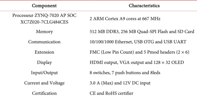
Zedboard platform [38] (Table 3) is an evaluation platform based on a Zynq-7000 family [39]. It contains on the same chip two components. The first is a dual-core ARM Cortex MPCore based on a high-performance processing system (PS). It can be used under Linux operating system or in a standalone mode. The second is an advanced programmable logic (PL) from the Xilinx 7th family that can be used to hold hardware accelerators in multiple areas. The two parts (PS and PL) interact between them by using different interfaces and other signals through over 3000 connections. Available four 32/64-bit high-performance (HP) Advanced eXtensible Interfaces (AXI) and a 64-bit AXI Accelerator Cohe-rency.

7.2. Test Sequences

As an effort to carry out a good evaluation of the standard, the JCT-VC devel-oped a document with some reference sequences and the codec configuration,

0 0.05 0.1 0.15 0.2 0.25 0.3

0 20 40 60 80 100

Probability

DOI: 10.4236/ijcns.2017.1011016 274 Int. J. Communications, Network and System Sciences Table 3. Zed board technical specifications.

Component Characteristics

Processeur ZYNQ-7020 AP SOC

XC7Z020-7CLG484CES 2 ARM Cortex A9 cores at 667 MHz

Memory 512 MB DDR3, 256 MB Quad-SPI Flash and SD Card Communication 10/100/1000 Ethernet, USB OTG and USB UART

Extension FMC (Low Pin Count) and 5 Pmod headers (2 × 6) Display HDMI output, VGA output and 128 × 32 OLED Input/Output 8 switches, 7 push buttons and 8leds

Current and Voltage 3.0 A (Max) and 12V DC input Certification CE and RoHS certifier

which should be used with each one [35]. The sequences are divided into 6 groups (Classes) based on their temporal dynamics, frame rate, bit depth, reso-lution, and texture characteristics

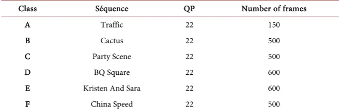
A subset of six video sequences was selected from this list. These six video se-quences were selected from classes A to F. Detailed descriptions of the sese-quences are given in Table 4.

7.3. The SDF3 Tool

The open-source SDF3 tool set [40] used in this work offers an SADF graph generation algorithm that constructs random SADF graphs, which are con-nected, consistent, and deadlock-free. This generation algorithm can be used to benchmark novel SADF analysis, transformation, and implementation algo-rithms. The user can restrict relevant properties of the generated graph (e.g., limit port rates, or construct only acyclic or strongly connected graphs). A set of command line tools as well as a C/C++ API implemented all algorithms used. The rich set of algorithms offered by SDF3, makes it a versatile tool set for the development of novel dataflow-based design approaches.

DOI: 10.4236/ijcns.2017.1011016 275 Int. J. Communications, Network and System Sciences Table 4. Test sequences used on experimentations.

Class Séquence QP Number of frames

A Traffic 22 150

B Cactus 22 500

C Party Scene 22 500

D BQ Square 22 600

E Kristen And Sara 22 600

F China Speed 22 500

worst-case scenario at any stage of the analysis. The constraint that the SDF graph must respect is the bit rate that must not be below 25 frames per second. Therefore, 25 iterations per second because the decoder decompresses an image by iteration. The value of the constraint will therefore be 0.025 iterations pertime unit (ms).

7.4. Actor’s Execution Times and Space Memory

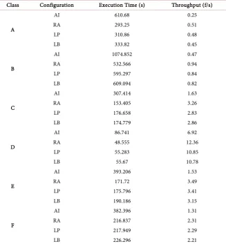
Execution times of actors are the first information needed for the modeling. It is expressed in abstract time units used by the sdf 3 flow command. The designer is thus free to map this abstract unit to a “manly” unit. The time unit used in this work is the processor cycle. To get actors’ execution times, several techniques are used. Some techniques use WCET tools or binaries; other uses simulation and other uses measurement and experimentations. In this work, we have done sev-eral profiling experimentations on the target platform (Zedboard) to calculate the WCET of each actor. Table 5 presents sequences execution time and throughput for all classes on the Zed board platform. Figure 7 presents the indi-vidual execution times for actors of HEVC Decoder (HM test model applica-tion).

In the rest of this paper, we present the experimental values applied to bits of class C (832 × 480 pixels).

We will work with the largest execution time for the AI configuration (worst case), which is equal to 307.414 seconds, and after division on 500 we will have 0.615 seconds (615 ms). In Tables 6-8, we present actors execution time, size of memory and size of tokens exchanged between actors for AI configuration.

For the RA, LD, LP configurations, the largest execution time of the three configurations is 176.658 seconds and after division on 500 will have 0.3533 seconds (354 ms), Actors Execution time (ms)-RA/LP/LB configuration

The memory space sizes for RC, MC, IP, SAO and DB are 400,000 bytes be-cause they manipulate variables that contain whole frames while the remainders are 5000 bytes because they only manipulate CTUs and then their variables are smaller.

DOI: 10.4236/ijcns.2017.1011016 276 Int. J. Communications, Network and System Sciences Table 5. Sequences execution time and throughput for all classes on the Zedboard plat-form.

Class Configuration Execution Time (s) Throughput (f/s)

A

AI 610.68 0.25

RA 293.25 0.51

LP 310.86 0.48

LB 333.82 0.45

B

AI 1074.852 0.47

RA 532.566 0.94

LP 595.297 0.84

LB 609.094 0.82

C

AI 307.414 1.63

RA 153.405 3.26

LP 176.658 2.83

LB 174.779 2.86

D

AI 86.741 6.92

RA 48.555 12.36

LP 55.283 10.85

LB 55.67 10.78

E

AI 393.206 1.53

RA 171.72 3.49

LP 175.796 3.41

LB 190.186 3.15

F

AI 382.396 1.31

RA 216.837 2.31

LP 217.949 2.29

LB 226.296 2.21

The SDF3 tool requires an xml file that describes all information collected from profiling step (such memory sizes, actors execution times, scenarios, tran-sitions between scenarios…). It is essential to adapt this information to the syn-tax imposed by the sdf3 because there are many rules to follow:

- Sizes must be in bytes.

- A same unit of time must be used along the description. - The execution times introduced are just for a single iteration.

The extension of SDF, FSM-based-SADF, which we exploited in our work, requires that the values introduced in the XML description of the application are values that describe the worst case.In this case, the measurement and estimation results in terms of bit rate (throughput) and memory space provided by SDF3 will never be exceeded even if there are other applications that run simulta-neously on the same platform.

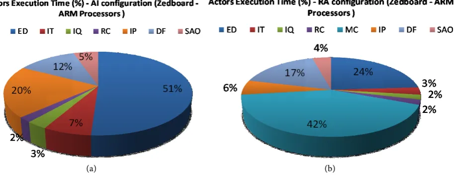
DOI: 10.4236/ijcns.2017.1011016 277 Int. J. Communications, Network and System Sciences (a) (b)

Figure 7. Percentages of execution time for each actor (for AI and RA configuration).

Table 6. Actors Execution time (ms)—AI configuration.

(a)

ED RC IQ IT MC IP DF SAO

313.56 12.30 18.44 43.04 inactif 122.97 73.78 30.74

(b)

ED RC IQ IT MC IP DF SAO

84.80 7.07 7.07 10.60 148.39 21.20 60.06 14.13

Table 7. Sizes of memory spaces consumed to store the internal state of each actor (byte).

ED RC MC IQ IT DB IP SAO

5000 400,000 400,000 5000 5000 400,000 400,000 400,000

Table 8. Sizes of tokens (byte).

DE2IQ DE2MC DE2IP DE2SAO IQ2IT IT2RC TA23DF DF2SAO MC2RC SAO2MC TA23IP IP2RC 16,384 12 16,384 5 16,384 16,384 1,597,440 1,597,440 1,597,440 1,597,440 1,597,440 1,597,440

Table 9 presents the values of rates according to the execution scenario. Y is the number of CTUs that are the references in an I frame. i.e. CTUs that will be used to generate the others (they will be passed in the residue). X is the number of blocks that have motion vectors. So (1560-x) is the number of CTUs that will be passed in the residue (case of frames of types P and B).

Table 10 illustrates the throughput variation of the decoding application ac-cording to the available memory size.

When we increase the memory space dedicated to input output channels for different actors, the throughput increases.

8. Conclusions

DOI: 10.4236/ijcns.2017.1011016 278 Int. J. Communications, Network and System Sciences Table 9. Scenarios.

Scenarios

Iy BPx

a Y 1560 – x

b 0 X

c 1 0

d 1 0

Table 10. Throughputs variation.

Total memory size (MB) Throughput (frame/s)

0.85379 5.1

21.099652 5.1

21.09975 5.1

21.427566 5.1

21.427622 5.1

21.755438 5.1

312.548904 64.5

312.630914 64.5

312.794898 64.5

312.958882 64.5

313.122866 64.5

313.28685 64.5

521.159654 106.1

521.323638 106.1

521.487622 106.1

521.651606 106.1

521.81559 106.1

521.979574 106.1

729.852378 147.7

730.016362 147.7

730.180346 147.7

730.34433 147.7

730.508314 147.7

730.672298 147.7

938.545102 189.3

938.709086 189.3

938.87307 189.3

939.037054 189.3

939.201038 189.3

DOI: 10.4236/ijcns.2017.1011016 279 Int. J. Communications, Network and System Sciences Functional Model MF(describing the application behavior), Architecture Model AM (describing the platform targets in number of processors, cache memory, communication system Bus/NoC), Constraint Model CM and Performance Model PM (execution time representation). The two new models introduced are the PM and the CM. The Constraint Model (CM) describes the functional con-straints of the application and non-functional concon-straints of the target platform. The Performance Model PM describes a performance evaluation of system in every abstraction level. An extension of Khan’s model is used. It is based on ad-dition of relative annotations to execution times and to the size of the data ex-changed of the parallel model.Experimentation is achieved, in this context, on the HEVC/h.265 decoder and the Zedboard platform of Xilinx.

The HEVC/h.265 video decoder is modeled with SADF based FSM in order to solve problems of placing and scheduling this application on an embedded ar-chitecture. This is done by identifying actor dependencies, number of data ex-changed (tokens), execution time and space memory of the decoder applied on C class of bitstreams.

A high-level performance analysis is performed to find an optimal balance between the decoding efficiency and the implementation cost allowing for a complexity reduction at a system level. For an optimal use of the HEVC tools, the best configuration parameters are obtained. For this cost-efficient configura-tion, the absolute complexity values, the memory and task level profiling results confirmed the big challenge needed for its effective implementation. For such implementation, a multiprocessor approach is needed to share the decoding ap-plication execution time between several processors for achieving better execu-tion performances and real time decoding.

References

[1] Jantsch, A. and Sander, I. (2005) Models of Computation and Languages for Em-bedded System Design. Computers and Digital Techniques, 152, 114-129.

[2] Lee, E.A. and Neuendorffer, S. (2005) Concurrent Models of Computation for Em-bedded Software. Computers and Digital Techniques, 152, 239-250.

[3] Hopcroft, J. and Ullman, J. (1979) Introduction to Automata Theory, Languages, and Computation. Addison-Wesley Publishing Company, Reading.

[4] Lee, E. and Messerschmitt, D. (1987) Synchronous Data Flow. IEEE Proceedings, 75, 1235-1245.

[5] Sriram, S. and Bhattacharyya, S.S. (2000) Embedded Multiprocessors: Scheduling and Synchronization. Marcel Dekker, Inc., New York.

[6] Bhattacharyya, S.S., Deprettere, F., Leupers, R. and Takala, J. (2013) Handbool of Signal Processing System. London.

[7] Stuijk, S. (2007) Predictable Mapping of Streaming Applications on Multiproces-sors. PhD Thesis, Eindhoven University of Technology.

DOI: 10.4236/ijcns.2017.1011016 280 Int. J. Communications, Network and System Sciences [9] Bennour, I., Sebai, D. and Jemai, A. (2010) Modeling SW to HW Task Migration for

MPSOC Performance Analysis.DTIS.

[10] Mesman, K.B., Theelen, B., Corporaal, H. and Ha, Y. (2008) Analyzing Composa-bility of Applications on MPSoC Platforms. Journal of Systems Architecture, 54, 369-383.

[11] Wiggers, M.H., Kavaldjiev, N., Smit, G.J.M. and Jansen, P.G. (2005) Architecture Design Space Exploration for Streaming Applications through Timing Analysis. Centre for Telematics and Information Technology, University of Twente, En-schede, Technical Report TR-CTIT-05-36.

[12] Shabbir, A., Kumar, A., Stuijk, S., Mesmana, B. and Corporaal, H. (2010) CAMP-SoC: An Automated Design Flow for Predictable Multi-Processor Architectures for Multiple Applications. Journal of Systems Architecture—Embedded Systems De-sign, 56, 265-277.

[13] Geilen, M. (2010) Synchronous Dataflow Scenarios. ACM Transactions on Embed-ded Computing Systems, 10, 16:1-16:31.

[14] Stuijk, S., et al. (2011) Scenario-Aware Dataflow: Modeling, Analysis and Imple-mentation of Dynamic Applications. 11th International Conference.

[15] Phan, L.T.X., Chakraborty, S. and Thiagarajan, P.S. (2008) A Multi-Mode Real-Time Calculus. Proceedings of the 2008 Real-Time Systems Symposium, Washington DC, 59-69.

[16] Thiele, L. and Stoimenov, N. (2009) Modular Performance Analysis of Cyclic Da-taow Graphs. Proceedings of the 7th ACM International Conference on Embedded Software, New York, 127-136.

[17] Theelen, B.D., Geilen, M., Basten, T., Voeten, J., Gheorghita, S.V. and Stuijk, S. (2006) A Scenario-Aware Data Model for Combined Long-Run Average and Worst-Case Performance Analysis. Memocode, 185-194.

[18] Poplavko, P., Basten, T. and van Meerbergen, J. (2007) Execution-Time Prediction for Dynamic Streaming Applications with Task-Level Parallelism. Proceedings of the 10th Euromicro Conference on Digital System Design Architectures, Methods and Tools, Washington DC, 228-235.

[19] Geilen, M. (2009) Synchronous Dataflow Scenarios. Transactions on Embedded Computing Systems, Special Issue on Model-Driven Embedded-System Design. [20] Ehrlich, P. and Radke, S. (2013) Energy-Aware Software Development for

Embed-ded Systems in HW/SW Co-Design.16th International Symposium on Design and Diagnostics of Electronic Circuits & Systems.

[21] Kai, H., Xio-xu, Z., Si-wen, X., et al. (2015) Profiling and Annotation Combined Method for Multimedia Application Specific MPSoC Performance Estimation. Springer-Verlag, Berlin, Heidelberg.

[22] Smei, H., Smiri, K. and Jemai, A. (2017) Profiling of HEVC Decoder Application in a Co-Design flow. 6th International Colloquium in Applied Research and Technol-ogy Transfer.

[23] Kahn, G. (1974) The Semantics of a Simple Language for Parallel Programming. Information Processing 74: Proceedings of the IFIP Congress 74, Stockholm, Au-gust 1974, 471-475.

[24] Bebelis, V. (n.d.) Boolean Parametric Data Flow. Streaming Day, V. BEBELIS (INRIA) BPDF. http://streaming.conf.citi-lab.fr/streaming_bebelis.pdf

DOI: 10.4236/ijcns.2017.1011016 281 Int. J. Communications, Network and System Sciences [26] Wauters, P., Engels, M., Lauwereins, R. and Peperstraete, J.A. (1996)

Cyc-lo-Dynamic Dataflow. Parallel and Distributed Processing.

[27] Lee, E.A. and Messerschmitt, D.G. (1987) Synchronous Data Flow. Proceedings of IEEE, 75, 1235-1245.

[28] Lee, E.A. and Messerschmitt, D.G. (1987) Static Scheduling of Synchronous Data Flow Programs for Digital Signal Processing. IEEE Transactions on Computers, 36, 24-35.

[29] Design and Implementation of Next Generation Video Coding Systems (H.265/HEVC Tutorial), Vivienne Sze, ISCAS Tutorial, 2014.

[30] Smei, H. and Jemai, A. (2016) Pipelining the HEVC Decoder on ZedBoard Plat-form. International Design & Test Symposium IDT.

[31] Wiegand, T., et al. (2003) Overview of the H.264/AVC Video Coding Standard. IEEE Transactions on Circuits and Systems for Video Technology, 13, 560-576. [32] Valgrind Web. http://valgrind.org/

[33] https://sourceware.org/binutils/docs-2.16/gprof/

[34] https://wiki.gnome.org/Apps/MemProf

[35] Bossen, F. (2012) Common Test Conditions and Software Reference Configura-tions. 9th Meeting of the JCT-VC in Geneva.

[36] BSD Licence HEVC Decoder (HM). https://hevc.hhi.fraunhofer.de

https://github.com/bbc/vc2-reference

[37] Theelen, B.D., Geilen, M.C.W., Stuijk, S., Gheorghita, S.V., Basten, T., Voeten, J.P.M. and Ghamarian, A.H. (2008) Scenario-Aware Dataflow, ES Reports.

[38] Zedboard Plateform. http://www.zedboard.org

[39] Xilinx, Inc. Zynq-7000 All Programmable SoC Technical Reference Manual. http://www.xilinx.com/support/documentation/user_guides/ug585-Zynq-7000-TR M.pdf