Tensor networks and geometry for the modelling of disordered quantum many body systems

(1)

University of Warwick institutional repository:

http://go.warwick.ac.uk/wrap

A Thesis Submitted for the Degree of PhD at the University of Warwick

http://go.warwick.ac.uk/wrap/70003

This thesis is made available online and is protected by original copyright.

Please scroll down to view the document itself.

(2)

Tensor Networks and Geometry for the Modelling

of Disordered Quantum Many-Body Systems

by

Andrew M Goldsborough

Thesis

Submitted to the University of Warwick

for the degree of

Doctor of Philosophy

Physics

(3)

List of Figures

2.1 Infinite system DMRG . . . 7

2.2 Diagrams of a vector, matrix and tensor . . . 11

2.3 Tensor network contractions . . . 12

2.4 MPS bra and ket diagrams . . . 13

2.5 Tensor reshaping . . . 14

2.6 Tensor contraction . . . 15

2.7 Contraction cost . . . 16

2.8 MPS canonical form . . . 19

2.9 Left and right normalisation of MPS tensors . . . 20

2.10 MPS with mixed normalisation . . . 21

2.11 MPS normalisation . . . 22

2.12 Construction of left block . . . 23

2.13 MPS density operators . . . 24

2.14 Expectation value for a single site operator . . . 26

2.15 Expectation value for operators acting on all sites . . . 27

2.16 MPO derivation . . . 29

2.17 MPS MPO expectation value . . . 30

2.18 Matrix product diagrams for nearest neighbour MPO . . . 32

2.19 Matrix product diagram for nearest neighbour MPO with on-site term 33 2.20 Matrix product diagram of next-to-nearest neighbour MPO . . . 34

2.21 Matrix product diagram for exponentially decaying MPO . . . 35

2.22 Matrix product diagrams for Heisenberg Hamiltonian . . . 37

2.23 Right normalising an MPS . . . 41

2.24 DMRG left and right blocks . . . 42

2.25 DMRG effective Hamiltonian . . . 43

2.26 DMRG algorithm . . . 44

2.27 Infinite two-site MPS DMRG . . . 45

(8)

2.29 Next site prediction in two site DMRG . . . 47

2.30 Density matrices from MPS tensors . . . 48

2.31 Modified density matrix . . . 49

2.32 Eigenvalue equation for OBCs . . . 50

2.33 Matrix product diagrams for nearest neighbour MPO with PBC . . 52

2.34 Matrix product diagrams for the Heisenberg Hamiltonian with PBC 53 2.35 MPS and MPO with PBC . . . 54

2.36 Matrix product diagram of a four site Hamiltonian MPO with PBC 55 2.37 Effective Hamiltonian with PBC . . . 56

3.1 Two-point correlation function from CFT . . . 62

3.2 Entanglement spectrum and entropy for the phases . . . 64

3.3 Previous phase diagrams for the disordered Bose-Hubbard model at N/L= 1 . . . 65

3.4 Phase diagrams for the disordered Bose-Hubbard model atN/L= 1 66 3.5 Finite size scaling of the Luttinger parameter K forN/L= 1 . . . . 67

3.6 Finite size scaling of the Mott gap Eg forN/L= 1 . . . 69

3.7 Previous phase diagram for the disordered Bose-Hubbard model at N/L= 1/2 . . . 70

3.8 Phase diagrams for the disordered Bose-Hubbard model atN/L= 1/2 71 3.9 Finite size scaling of the Luttinger parameter K forN/L= 1/2 . . . 72

3.10 Superfluid fraction ρs(U) at ∆µ= 0.5 for N/L= 1/2 . . . 73

3.11 Average maximum filling over the N/L= 2 phase diagram . . . 74

3.12 Phase diagrams for the disordered Bose-Hubbard model atN/L= 2 75 3.13 Finite size scaling of the Luttinger parameter K forN/L= 2 . . . . 76

3.14 Finite size scaling of the Mott gap Eg forN/L= 1 . . . 77

4.1 Singular values from DMRG . . . 80

4.2 Correlation functions from DMRG . . . 81

4.3 Geometry of an MPS . . . 82

4.4 Geometry of a PEPS . . . 83

4.5 The corner of Hilbert space . . . 84

4.6 Entanglement and correlation in AdS/CFT . . . 85

4.7 Geometry of a periodic MERA . . . 87

5.1 SDRG algorithms of MDH, Westerberg and Hikihara . . . 89

5.2 Tensor network diagrams for SDRG as an MPO process . . . 92

(9)

5.4 The SDRG algorithm as a TTN . . . 95

5.5 Commutativity of isometries . . . 96

5.6 Indexing in tSDRG . . . 97

5.7 Correlation functions in tSDRG . . . 99

5.8 Density matrix and reduced density matrix in tSDRG . . . 100

5.9 Efficient calculation of density matrix in tSDRG . . . 102

5.10 Ground state energy per site . . . 103

5.11 Spin-spin correlation function . . . 104

5.12 Scaling parameter as a function of L . . . 106

5.13 Typical spin correlation function . . . 107

5.14 Fit of tensor network geometry to correlation function . . . 108

5.15 Entanglement entropy as a function of disorder . . . 109

5.16 Entanglement as a function of system size . . . 110

5.17 Entanglement entropy as a function of block size . . . 111

5.18 Entanglement entropy per bond . . . 112

6.1 Definitions for complete trees . . . 116

6.2 Decomposition of a tree into two primary subtrees . . . 117

6.3 Average leaf-to-leaf path length for complete binary tree . . . 119

6.4 Average leaf-to-leaf path length for infinite m-ary trees . . . 122

6.5 Variance for binary trees . . . 124

6.6 Variance for infinite m-ary trees . . . 125

6.7 A complete, periodic binary tree . . . 129

6.8 Correlation function for homogeneous complete TTN . . . 131

7.1 Definitions for Catalan trees . . . 135

7.2 All unique binary trees with 1, 2 and 3 vertices . . . 136

7.3 Diagrammatic decomposition of the set on trees withn vertices . . . 136

7.4 Diagrammatic decomposition for the first leg . . . 140

7.5 Diagrammatic decomposition for the second leg . . . 141

7.6 Nearest neighbour path length in annvertex tree . . . 151

7.7 The connecting paths forr= 3 . . . 155

7.8 Bulk and boundary contributions to the path length . . . 155

7.9 Symmetry between short and long paths . . . 156

7.10 Legs involved in boundary paths . . . 157

7.11 Equivalence between path lengths and rooted paths . . . 163

7.12 Average path length as a function of separation . . . 164

(10)

7.14 Path length as a function of separation for random binary trees . . . 166

7.15 Comparing paths in the different trees . . . 167

A.1 String theory? . . . 175

A.2 Path to depth correspondence forn= 3 . . . 176

(11)

Acknowledgments

Scientific research is never performed in a bubble, we rely so much on those around

us for support, inspiration and distraction, without which getting to the point of

submitting a PhD thesis would be impossible. I have a lot of people to thank and I

have no doubt that I have missed a great many more.

First and foremost I would like to thank my supervisor Prof. Rudolf A.

R¨omer for giving me the opportunity to live a life of science. He somehow

man-aged to balance both guidance and freedom to pursue my own research interests,

providing a wealth of knowledge on both physics and general life that will no doubt

be influential in my future decisions. On the technical side I would like to thank

the Engineering and Physical Science Research Council (EPSRC) for financial

sup-port (EP/J003476/1) and the MidPlus Regional HPC Centre (EP/K000128/1) for

computing resources that were used to perform my research.

On a more personal level I would like to thank my fellow students in PS001

and members of the Warwick theory group notably: Matthew Bates, Dr. Jack Heal,

Anja Humpert, Dr. Daniel Pearce, Dr. Sebastian Pinski and Alex Rautu to name but

a few, for creating such an enjoyable and friendly working atmosphere, always being

there to talk science or anything but. I would like to thank the coauthors of the graph

theory work. The path length problem was originally something fun to try before

going to the pub on a Friday afternoon, but turned out to be a fantastic learning

experience. I would also like to thank the great many scientists from around the

world whom I have met and become friends with at conferences and workshops. In

many ways it is the people who make science such a unique and enjoyable enterprise.

(12)

col-lectively known as theKnights of Ni (KON) for all of the adventures over the years.

My friends from the Michael Stoker Building (MSB) at Clare Hall, Cambridge for

the good food and the good times. Dr. Mark Pinder for friendship and school bus

discussions on science and philosophy that instilled a passion and thirst for

knowl-edge that is yet to be diminished. My friend and flatmate Dr. David Dossett for

friendship and guidance in some of the most stressful of times. My parents Alan

and Janet, and brother Mark for unending support at every point in my life and

making me the person that I am.

Finally, a special thanks go to my girlfriend Steph who has been so loving,

(13)

Declarations

I declare that the content of this thesis is original work except where referenced

within the text and has not been submitted as part of any other degree or

qualifi-cation. Chapters 1, 2 and 4 provide a background to the field, the information for

which was gathered from the texts cited throughout. Chapters 3, 5, 6 and 7 are

respectively based on the following papers:

• A. M. Goldsborough and R. A. R¨omer. Using entanglement to discern phases

in the disordered one-dimensional Bose-Hubbard model. arXiv:1503.02973

[cond-mat.dis-nn], March 2015, (submitted to EPL).

• A. M. Goldsborough and R. A. R¨omer. Self-assembling tensor networks and

holography in disordered spin chains. Phys. Rev. B, 89:214203, June 2014.

• A. M. Goldsborough, S. A. Rautu, and R. A. R¨omer. Leaf-to-leaf distances

and their moments in finite and infinite m-ary tree graphs. Phys. Rev. E,

91:042133, April 2015.

• A. M. Goldsborough, J. M. Fellows, S. A. Rautu, M. Bates, G. Rowlands, and R. A. R¨omer. Leaf-to-leaf distances in ordered Catalan tree graphs.

arXiv:1502.07893 [math-ph], February 2015, (in preparation).

The entirety of the work was conducted under the supervision of Professor R. A.

R¨omer and the content of the chapters highlighted above was performed in

collab-oration with the indicated authors. The thesis was typeset with LA_{TEX 2ε} _{and the}

warwickthesis style using the Vim text editor. Graphs were drawn using XMGrace

(14)

Abstract

This thesis explores the use of tensor networks in the study of disordered quantum-many body systems and the connection between disorder in the Hamilto-nian and tensor network geometry.

Tensor networks provide a powerful and elegant approach to quantum many-body simulation. The simplest example is the density matrix renormalisation group (DMRG), which is based on the variational update of a matrix product state (MPS). It has proved to be the most accurate approach for the numerical study of strongly correlated one dimensional systems. We use DMRG to study the one dimensional disordered Bose-Hubbard model at fillings N/L= 1/2, 1 and 2 and show that the whole phase diagram for each can be successfully obtained by analysing entangle-ment properties alone. We find that the average entangleentangle-ment is insufficient to accurately locate all of the phases, however using the standard error on the mean we are able to construct a phase diagram that is consistent with previous studies.

It has recently been shown that there is a connection between the geometry of tensor networks and the entanglement and correlation properties that it can encode, which is a generalisation of the so calledarea law for entanglement entropy. This suggests that whilst gapped quantum systems can be accurately modeled using an MPS, a tensor network with a holographic geometry is natural to capture the logarithmic entanglement scaling and power law decaying correlation functions of critical systems. We create an algorithm for the disordered Heisenberg Hamiltonian that self assembles a tensor network based on the disorder in the couplings. The geometry created is that of a disordered tree tensor network (TTN) that when averaged has the holographic properties characteristic of critical systems.

(15)

Abbreviations

AdS -Anti-de Sitter space

AdS/CFT -Anti-de Sitter/conformal field theory correspondence

AFM -Antiferromagnetic

APBC -Anti-periodic boundary condition

CFT -Conformal field theory

DMRG -Density matrix renormalisation group

FM -Ferromagnetic

KT - Kosterlitz-Thouless

MBL -Many-body localisation

MDH -Ma, Dasgupta and Hu

MERA -Multi-scale entanglement renormalisation ansatz

MPO -Matrix product operator

MPS -Matrix product state

NRG -Numerical renormalisation group

OBC -Open boundary condition

PBC - Periodic boundary condition

PEPS -Projected entangled pair state

QMC - Quantum Monte Carlo

RG -Renormalisation group

SDRG -Strong disorder renormalisation group

SVD -Singular value decomposition

tSDRG -Tree tensor network strong disorder renormalisation group

(16)

Chapter 1 Introduction

At its most basic level a quantum many-body system can be defined by a Hilbert space and a Hamiltonian which can describe the evolution of the state. The

di-mension of the Hilbert space grows exponentially with the number of particles in

the system. Calculations for systems containing a small handful of particles can be simple, but the exponential scaling means that exact calculations quickly become

unfeasible. As a simple example take a spin-1/2 system, where each particle can

take one of two states. Because of the tensor product form of the Hilbert space, the dimension scales as 2n _where _n _{is the number of particles [1]. For one mole of}

such particles, the dimension and therefore the number of states is ∼ 21023. Thus the number of possible states in just one mole of these simplified particles dwarfs the total number of particles in the universe [2], which is estimated to be ∼1080.

This highlights part of the problem in modelling quantum matter; any attempt to

perform a calculation for a reasonably large number of particles fails spectacularly. The exponential growth of Hilbert space has led to some scholars questioning not

just the impracticiality of such a large space, but even if such a construction is

physical [3, 4].

As exact calculations for quantum many-body systems are not possible, it is

necessary to use methods that reduce computational complexity whilst still

achiev-ing high accuracy. There have been several numerical algorithms that have enabled the simulation of materials that would have otherwise been impossible. For large

scale electronic sturctures, like those found in condensed matter physics and

quan-tum chemistry, dynamical mean field theory (DMFT) and density functional theory (DFT) have been very successful, but are limited to systems without significant

(17)

the properties of physical system can be determined from the electron density of

the ground state, which can be determined from an effective non-interacting sys-tem [6]. Wilson’s numerical renormalisation group (NRG) [7], as will be discussed

in chapter 2, trucates the Hilbert space using the low energy eigenvectors of the

Hamiltonian. It is used primarily on impurity models, and is not at all successful as a general approach to quantum many-body problems. Quantum Monte Carlo

(QMC) is perhaps the most well known method, this maps a quantum problem ind

spatial dimensions to that of ad+ 1 dimensional classical partition function [8]. One of the major issues with QMC is thesign problem, which prevents the method from

being successful for many frustrated and fermionic systems. In these cases the

map-ping to the classical system introduces negative Boltzmann weights that make the statistical error quickly become larger than the property being calculated [8]. A new

method created in 1992 by White, called thedensity matrix renormalisation group,

revolutionised the simulation of one dimensional systems. It truncates the Hilbert space in accordance with the eigenstates corresponding to the largestχeigenvalues

of the ground state density matrix. Because of the use of the density matrix, rather

than just the eigenvectors of the Hamiltonian as in NRG, DMRG encodes some of the entanglement of the ground state allowing accurate simulation of many

quan-tum systems. Unlike QMC, DMRG does not suffer from the sign problem and is considered the most accurate numerical method for one dimensional systems [9].

Disordered quantum many-body systems are of great interest but are

partic-ularly problematic. It is natural to want to study systems with disorder as perfect clean materials are very rare in nature. Furthermore the introduction of disorder

can completely change the observed phase of the material. The study of disordered

systems became a major part of the study of the electronic properties of condensed matter with the analysis of localisation by Anderson [10]. For non-interacting

elec-tronic systems in a three dimensional disordered lattice it was found that a critical

value of the on site disorder marked the transition between extended and localised states. The interplay between interactions and disorder is much less well understood

andmany-body localisation is currently a hot topic of research.

In this thesis we will analyse the theory oftensor networks, and apply them with a focus on disordered systems. In chapter 2 we introduce the basic concepts of

a tensor network in the context of DMRG. We provide all information necessary to

understand the fundamental operations that make up a tensor network algorithm and use them to construct the matrix product state (MPS), which is the simplest

example of a tensor network. We show how to perform a variational update to the

(18)

of MPS DMRG we analyse the disordered Bose-Hubbard model in chapter 3. As

entanglement is at the heart of DMRG and is calculated at every point in the simulation of the system, we illustrate the efficacy of entanglement as a tool for

deciphering the phase of the ground state wavefunction. The content of this chapter

is based on ref. [11], which is currently under review. In chapter 4 we discuss more generally the theory of tensor networks, why they work for certain cases and

why they don’t for others and how tensor networks go beyond DMRG to simulate

more complex systems. Chapter 5 creates a tensor network algorithm where the structure of the network is determined by the disorder in the Hamiltonian. In this

way each disorder realisation has a custom tree tensor network (TTN) and when

disorder averaged we show that the system has holographic properties that govern the entanglement and correlation scaling. The chapter is based on [12], which was

published in Physical Review B. The final two chapters (6 and 7) analyse how the

geometry of tree tensor networks affects the asymptotic form of the averaged two-point correlation function. Chapter 6 looks at a complete tree and finds the average

leaf-to-leaf path length when the leaves of the tree are effective lattice points. This

chapter is based on [13], which is currently under review. Chapter 7 extends the ideas of the previous chapter to sets of full binary trees that are more similar to

(19)

Chapter 2 Matrix Product States and the

Density Matrix Renormalisation

Group

2.1 White’s Density Matrix Renormalisation Group

The field of tensor networks has its roots in Wilson’s NRG [7] and the DMRG

method devised by White [15]. As mentioned in chapter 1, for an interacting one

dimensional system ofLsites, the Hilbert space of the system is the product of the Hilbert spaces of the sites

HL=H ⊗. . .⊗ H. (2.1.1)

If each site can take one of n states, the Hilbert space of the system scales as nL_.

This exponential increase means that any computation quickly becomes intractable.

NRG and DMRG are numerical methods that reduce the size of this Hilbert space to a point that computations are possible, but still retains the necessary information

regarding the low energy eigenstates. As a motivation to the theory and application

of tensor networks we will briefly sketch out these two algorithms.

2.1.1 Numerical Renormalisation Group

The NRG algorithm famously worked well for the Kondo impurity model, which

maps a spherically symmetric Kondo model onto a lattice Hamiltonian with the

impurity as the first site and the conduction electrons as the rest of the lattice [16]. NRG is a purely numerical method and works by tracing out the higher energy

(20)

[16]:

1. Take L sites at the left hand side of the system to form a block, where L is

small enough so that the HamiltonianHL can be exactly diagonalised.

2. DiagonaliseHLand keep only themeigenvectors corresponding to the lowest

eigenvalues as the higher eigenvectors do not contribute significantly to the

ground state of the system.

3. Form a matrixO of the meigenvectors

O= 

   ..

. ... ...

V1 V2 . . . Vm

..

. ... ... 

  

(2.1.2)

whereV1 is the ground state eigenvector and so on.

4. UseO to change the basis and truncate the size of the Hamiltonian

¯

HL=O†HLO (2.1.3)

and all other operators

¯

AL=O†ALO (2.1.4)

These will now be matrices of dimensionm×m.

5. Add a site onto the block to formHL+1 and repeat the procedure from step 2

until the full length of the chain is reached.

This procedure works well because each successive site is less well coupled to the

impurity and thus the energy scale is lower. Most lattice problems (for example the

Heisenberg model) do not have these properties, and so NRG is not appropriate. It turns out that the solution to getting a successful procedure for a one dimensional

lattice system lies in the density matrix projection. Instead of using the lowestm

eigenstates to truncate the Hamiltonian matrix at each step, DMRG uses the lowest m eigenstates of the ground statedensity matrix to perform the truncation. Using

the density matrix does not necessarily choose the lowest energy eigenstates locally,

but rather the states that are mosthighly coupled to the ground state [17].

2.1.2 Infinite System DMRG Procedure

(21)

finite algorithm acts upon the superblock to accurately find the ground state of the

system. The infinite algorithm is [16, 18]:

1. Start with a superblock of sizeL= 4 that is made up of a left (system) block of sizel= 1;Hl, two single sites and a right (environment) block of sizel= 1;

H_lR.

2. Form Hl+1 and Hl+1R within the superblock.

3. Form the superblock fromHl+1 and Hl+1R .

4. Diagonalise the superblock and find the ground state eigenvector|ψi.

5. Create the density matrix

ρii0 = X

j

ψ∗_ijψi0_j. (2.1.5)

6. Diagonalise the density matrix and keep the eigenvectorsV corresponding to

the lowestm eigenvalues.

7. Create matrix O that will be used to truncate the operators:

O= 

   ..

. ... ...

V1 V2 . . . Vm

..

. ... ... 

  

(2.1.6)

8. UseO to change the basis and truncate the size of the Hamiltonian:

¯

Hl+1 =O†Hl+1O (2.1.7)

and all of the operators:

¯

Al+1 =O†Al+1O (2.1.8)

These will now be matrices of dimensionm×m.

9. Create a new superblock of sizeL+ 2 from ¯Hl+1, two sites and ¯Hl+1R .

10. Repeat from step 3 to grow the size of the superblock by two sites each

(22)

Superblock

2l+2

l+1 l+1

Construct superblock Insert two sites

L R

L

R

L

R

Diagonalise and truncate L and R

Repeat

Figure 2.1: Pictorial representation of the infinite DMRG process. Starting with the left (system) and right (environment) blocks, each representing l sites, two sites are added to create a superblock. This is diagonalised and the ground state eigenvector used to make a density matrix, the eigenvectors corresponding to the lowestmeigenvalues of which are used to truncate the Hamiltonians for the newLandRblocks representingl+1 sites. The whole process is then repeated.

2.1.3 Finite System DMRG Procedure

The finite system DMRG algorithm uses the same basic principles that are used in

the infinite algorithm, however the system is kept at a set sizeL and the aim is to calculate the energy of the desired state to a greater accuracy. The finite system

algorithm is usually used after the length of the chain has grown to a desired size

using the infinite algorithm. In the finite case the superblock is again constructed from a left (system) block, lengthl, two states and a right (environment) block, size

l0. Now the system and environment blocks are no longer kept the same size so that the location on the chain that the two sites are inserted moves along the chain. The algorithm is performed as follows:

1. Perform the infinite algorithm until the chain length is the desired size L

storing the ¯Hl, ¯HlR0 and all of the operatorsA_l that are required to construct

the superblock at each step.

(23)

4. Form a superblock from ¯Hl+1, two sites and ¯Hl0₋₁.

5. Proceed by performing steps 3 and 4 until the right hand edge of the system

is reached, wherel0= 1. This is the right sweep.

6. Now grow the right block at the expense of the left block. Perform steps 3

and 4 with the roles oflandl0 reversed until the left hand edge of the system is reached, wherel= 1. This is theleft sweep.

7. Again, reverse the roles ofland l0 and perform another left sweep.

8. Repeat, sweeping back and forth across the system until convergence is hit or

a specified number of sweeps is reached.

DMRG proved to be a highly accurate and versatile numerical method with

applications too numerous to list here, but comprehensive review articles provide

many references [9, 19]. It was discovered by ¨Ostland and Rommer [20] that DMRG can be interpreted as an MPS. The MPS allows a greater understanding of the

structure of information in the DMRG algorithm, giving reason for its successes and failures (see chapter 4). This has lead to further developments such as time

evolution [21, 22, 23], systems in the thermodynamic limit [24] and efficient periodic

boundary conditions (PBCs) [25, 26, 27]. The theory that has been developed in the context of MPS DMRG opens the door to more complex algorithms acting on

networks of tensors with structures designed to suit the problem at hand. All of

these tensor network algorithms have a lot in common with MPS DMRG, so the rest of this chapter will be devoted to a pedagogical overview of MPS.

2.2 Introduction to Matrix Product States

Consider a quantum system with basis states |↑i and |↓i. Simple states can be formed as a product of these [28], for example

|Ψi=|↑i ⊗ |↑i. (2.2.1)

In general these states can be written as a product of the two sites

(24)

Using summation notation this can be an outer product of two element vectors

|Ψi= X

σ1,σ2

Vσ1|σ1i ⊗Vσ2|σ2i

= X

σ1,σ2

Cσ1,σ2|σ1i ⊗ |σ2i, (2.2.3)

whereσi can be↑ or↓and Cσ1,σ2 is a two component tensor with elements

Cσ1,σ2 =

ac ad bc bd

!

. (2.2.4)

Product states such as these have the bases independent of each other and the expectation values factorise. On the other hand, entangled states such as

|Ψi= √1

2(|↑i ⊗ |↓i − |↓i ⊗ |↑i) (2.2.5)

do not have factorising expectation values. The maximally entangled state (2.2.5)

would require a tensor of the form

σ2 =↓ σ2=↑

σ1=↓ 0 −1/ √

2 σ1=↑ 1/

√

2 0

which cannot be described by eq. (2.2.4). If instead of being described by vectors,

letVσ1 and Vσ2 be matrices [29], for example

Mσ1,i=

1

4

√

2 1 0

0 1 !

, Mi,σ2 =

1

4

√

2

0 −1

1 0

!

(2.2.6)

These matrices are then combined using a standard matrix product over theiindex,

which gives the entangled state

X

i

Mσ1,iMi,σ2 =

1

√

2

0 −1

1 0

!

, (2.2.7)

as desired. Theiindex introduces entanglement between the two states and can be

(25)

Equation (2.2.2) can be generalised to a lattice ofLstates with open

bound-ary conditions (OBCs). Here, a product state is given by

|Ψi=

L

Y

i=1

[ai(↑)|↑ii+ai(↓)|↓ii], (2.2.8)

where there are two coefficients,ai(↑) andai(↓), for each site [28]. Equation (2.2.3)

is generalised to include anL index tensorCσ1...σL and the wavefunction becomes

|Ψi= X

σ1,...,σL

Cσ1...σL|σ1i ⊗ · · · ⊗ |σLi. (2.2.9)

As with the two particle case, theL index tensor can be split into a series of local

tensors with connections to their neighbours that allow the inclusion of

entangle-ment. When away from the boundaries each site has two neighbours thus the tensors at each site have three indices; one for the site basis and one for each neighbour. In

full the wavefunction takes the form

|Ψi= X

σ1,...,σL

X

a1,...,aL−1

Mσ1,a1Mσ2,a1a2. . . MσL−1,aL−2aL−1MσL,aL−1|σ1, . . . , σLi,

(2.2.10)

where|σ1. . . σLiis a short hand for|σ1i ⊗ · · · ⊗ |σLi. For the remainder of the thesis

the⊗ will be omitted for simplicity but is implied in the product of basis vectors.

The σi indices label the spins of the basis and are known as the physical indices,

whereas the ai are the bond, virtual or auxiliary indices. To draw a distinction

between the two index types it is convention to have the physicalσias upper indices,

thus giving the standard form of an MPS

|Ψi= X

σ1,...,σL

X

a1,...,aL−1

Mσ1

a1M

σ2

a1a2. . . M

σL

aL−2aL−1M

σL

aL−1|σ1, . . . , σLi. (2.2.11)

Taking the hermitian conjugate gives the bra state

hΨ|= X

σ1,...,σL

X

a1,...,aL−1

M∗σ1

a1 M

∗σ2

a1a2. . . M

∗σL−1

aL−2aL−1M

∗σL

aL−1hσ1, . . . , σL|. (2.2.12)

The MPS is a valuable tool in the computation of quantum many body states as, by

controlling the size of the matrices one can introduce enough entanglement to model a local Hamiltonian but keep the Hilbert space small enough such that calculations

are tractable. This is know as setting the bond dimension,χ, and within a DMRG

(26)

(a) (b) (c)

Figure 2.2: Diagrammatic representations of (a) a vector, (b) a matrix, and (c) a general tensor. The shape represents the object and the lines or legs

the indices.

the density matrix (see 2.1.2).

2.3 Diagrammatic Notation

One of the most elegant features of the tensor network formalism is the diagrammatic

representation of the mathematics, which makes visualising the algorithms very easy.

A tensor is drawn as a shape (here circles) where each index is represented by a line orleg. In this manner a vector, which is a one index tensor, is a circle with one line

coming from it. Similarly a matrix is a circle with two legs and a general tensor

withkindices is a circle with k legs. Examples of these are given in fig. 2.2. Multiplication of tensors is generalised by the notion of tensor contraction.

The simplest example is a vector inner product that takes two vectors to give a

scalar

S=X

i

ViVi0. (2.3.1)

In the tensor network diagrammatic convention the contraction is drawn by joining

the lines that represent the summed over index, resulting in a object with no legs as shown in fig. 2.3(a). Multiplication of a vector with a matrix is

V_j0 =X

i

ViMij, (2.3.2)

drawn in fig. 2.3(b). General contraction is the summation over the repeated index

of any two tensors, for example

Cij...i0_j0_...= X

k

Aij...k...Bi0_j0_...k..., (2.3.3)

(27)

there-(a)

=

(b)

=

(c)

=

Figure 2.3: Diagrammatic representations of contractions. (a) Inner prod-uct of a vector with another vector (eq. 2.3.1). (b) Vector multiplying a matrix (eq. 2.3.2). (c) General tensor contraction (eq. 2.3.3).

The standard diagram for an MPS is a chain of circles connected horizontally by the

bond indices with the physical indices drawn vertically. The MPS of eq. (2.2.11) is

given in fig. 2.4(a). The bra state MPS (2.2.12) will be drawn in a similar way to the ket but with the physical indices pointing in the opposite direction as shown in

fig. 2.4(b).

There is no set convention as to whether the physical indices for the wave-function should point up or down and the literature contains examples of both

(up: [29, 30, 31, 32, 33], down: [2, 34, 35, 36, 37, 38, 39, 40, 41]). Throughout

this document a ket state will have physical indices that point down to be con-sistent with the conventions of the literature on holographic tensor network states

[12, 34, 42, 43, 44, 45] that will become important in latter parts of the thesis.

2.4 Fundamental Details

Tensor networks require operations that manipulation the tensors, the most

funda-mental of which arereshaping and contraction. It is using these actions that all of the more complicated tensor network algorithms are built.

2.4.1 Tensor Reshaping

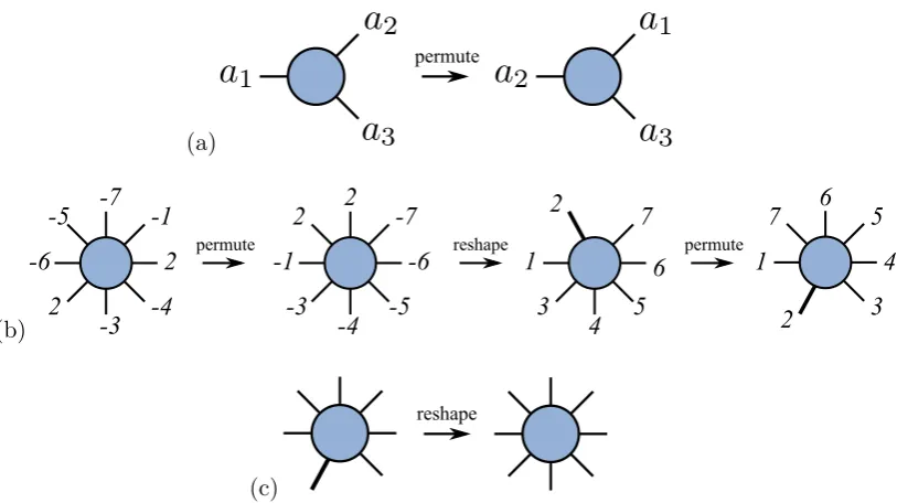
The reshaping of the tensors involves permutation, fusing and splitting of indices.

(28)

(a)

(b)

Figure 2.4: Diagrammatic representation of an MPS (a) ket given by eq. (2.2.11) and (b) bra given by eq. (2.2.12). The circles represent the M

tensors and the lines are the tensor indices. The horizontal lines represent the bond indices, the vertical lines the physical indices.

transpose operation on a matrix. For exampleAa1a2a3 _{can be permuted to} _Aa2a1a3

as shown by fig. 2.5(a). Permutation and limited reshaping functions for tensors are common and exist in packages such as MATLAB and NumPy, but general fusion

and splitting functions are not.

Fusion involves combining two or more indices to create a composite index that spans all combinations of the original indices, the following is a description of

how to create such a function and is shown diagrammatically in fig. 2.5(b). Begin

by labelling the indices of the tensor by the desired final order with the legs that are to be fused given a positive number, the indices to be left given a negative number.

The indices are then permuted to be in the order of the labels, with the convention that the diagrams are labelled from 9 o’clock anticlockwise as in [37]. Note that now

the two indices that are to be fused are next to each other. To fuse these indices

it is necessary to calculate the dimension of the resulting composite index, which is product of the component indices. The next step is to reshape the tensor into the

desired form. This is performed by flattening the tensor into a vector then splitting

it up into indices of the desired dimension (in MATLAB, for example, this is done by the reshape function) where the final index is now the composite index. The

final step is to permute the reshaped tensor such that the indices are in the desired

order. Here we note that the distinction between indices to be fused and not is no longer needed so the negative indices are made positive to allow the permutation to

be made in the correct order.

(29)

(a)

permute

(b)

1 3

4 7 2

6 5 -1

2

-3 -4 -7

2 -6

-5

-1 -3

-4 -5 -6 -7 2 2

permute reshape

1

3 4 7

2 6

5

permute

(c)

[image:29.595.125.532.104.332.2]

reshape

Figure 2.5: Example of (a) permutation of indices, (b) the tensor fusion function and (c) the tensor split function as described in the text.

will be split and the sizes of the desired component indices after splitting. Create a

list of the index dimensions for the tensor and insert the split dimensions in place of the dimension of the index to be split then reshape the tensor according to this

list of index sizes. This is diagrammatically shown in fig. 2.5(c). It is important

that the fuse and split have the same indexing convention such that splitting after a fusion recovers the same tensor. Note that MATLAB like Fortran iscolumn-major,

whereas NumPy like C and Mathematica isrow-major.

2.4.2 Tensor Contraction

The most commonly performed action in a tensor network algorithm is the tensor

contraction, so it is vital that it is done fast. As mentioned in section 2.3, the concept

of a tensor contraction is a generalisation of a matrix multiplication to objects of arbitrary dimension. Matrix multiplication algorithms are very common and there

exist very highly optimised functions in linear algebra packages such as BLAS and

LAPACK, which form the basis of the tensor contraction function. To use the matrix multiplication functions, the tensors must first be reshaped into matrices, multiplied

and then converted back into tensors.

(30)

1 -8

-1

-2

-3

-4

-7

-6

-5

1 -8

-1

-2

-3

-4

-7

-6

-5

fuse

multiply

6

5

3

4

7

2

1

8

2

3

5

1

4

7

6

permute

split

Figure 2.6: Diagrammatic form of the tensor contraction function as de-scribed in the text. Note that the minus signs are dropped after the multi-plication.

often many different ways that two tensors can be contracted depending on which

index is being summed over. Therefore in a similar manner to the fusion function, the contraction function requires instruction as to which indices to contract and the

desired order of the indices of the resulting tensor, where the indices to be contracted

are positive and those to be left are negative. Using the numbering, permute the tensors such that the indices to be contracted are the final indices on the left hand

tensor, A, and the first indices on the right hand tensor, B. Fuse the indices that

are not contracted on each tensor leaving two matrices, each with one index to be contracted. These matrices can then be efficiently multiplied resulting in a matrix,

C, with one index being a composite of the un-contracted indices ofAand the other

the un-contracted indices of B. These two legs are then split and permuted into the desired form. Similar to the fusion example, after multiplication there are no

indices to be contracted over therefore the negativity of the remaining indices can

be dropped so that the permutation achieves the desired result. Figure 2.6 shows a diagrammatic example of the mechanics of the tensor contraction.

2.4.3 Time Estimates

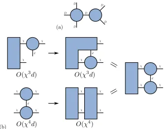
The order in which a tensor network is contracted can have a great effect on the execution time of an algorithm, therefore it is useful to have a means of estimating

this cost so that the optimal order of contraction can be found. The diagrammatic

(31)

(a)

[image:31.595.154.488.105.368.2]

(b)

Figure 2.7: Contraction of (a) two tensors with computational costing O(D6) and (b) Contraction of three tensors, showing that the order of contraction effects the cost of an operation.

example contraction of a rank four and a rank three tensor as shown in fig. 2.7(a)

where each index hasDelements is of order D6 orO(D6).

An simple example of where the order of contraction effects the overall cost

of an operation is shown in fig. 2.7(b). This is the contraction of two MPS tensors

with a left block, which is part of calculating an expectation value, the details of which are in section 2.5.4. The top order isO(χ3d), whereas the bottom is O(χ4d).

With an MPS the bond dimensionχcan be∼100 - 1000 so the second order takes

abouta thousand times longer, clearly showing the advantage of choosing an optimal order of contraction.

2.4.4 Singular Value Decomposition

Another commonly used tool in the manipulation of tensor network states is the

singular value decomposition (SVD) [30], which states that a rectangular matrixA

of dimensionNA×NB can always be written in the form

(32)

U is anNA×min(NA, NB) matrix with orthonormal columns (U†U =11), which is

unitary if NA = NB (U U† = U†U = 11). S is diagonal with non-negative entries,

which are the singular values and are usually given in order of decreasing size. V† is a min(NA, NB)×NBmatrix with orthogonal rows ((V†)(V†)†=11), which is also

unitary ifNA=NB.

For a system of more than two sites, with the bases split into two blocksA

and B with dimensions NA and NB respectively, a state of the system |Ψi can be

written as [30]

|Ψi=X

i,j

Ψij|σiiA|σji_B, (2.4.2)

where |σiiA and |σji_B are orthonormal bases of A and B respectively, and the

coefficients are elements of matrix Ψij. Performing an SVD of Ψij in eq. (2.4.2)

gives

|Ψi= X

i,j

Ψij|σiiA|σji_B

= X

i,j,a

UiaSaaVaj† |σiiA|σji_B, (2.4.3)

This is also known as aSchmidt decomposition.

The amount of entanglement between blocksA andB is encoded within the

singular values, which is quantified by thevon Neumann orentanglement entropy

S_A|B=−

X

a=1

s2_alog₂s2_a, (2.4.4)

wheresa are the singular values from diagonal matrixS. When the wavefunction is

normalised the set of singular values square and sum to 1. If only one of thesa is

non-zero, then the system is in a product state with SA|B = 0. The other extreme

is having all of the singular values equal, i.e. sa= 1/ √

N whereN is the dimension

of matrixS. This maximally entangled state therefore has entropy SA|B= log2N.

2.5 Matrix Product States

2.5.1 The Canonical Form

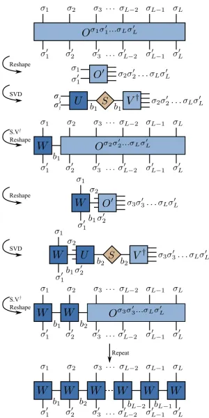
It is possible to take any state with tensorCσ1...σL _{and convert it into an MPS [30].}

The tensor is first reshaped into a matrix C_σ0[1]

1,(σ2...σL), where the second index is a

(33)

two by performing an SVD

Cσ1...σL ₌_C0[1]

σ1,(σ2...σL)=

X

a1

U_σ[1]₁_,a₁S_a[1]₁_,a₁V_a[1]†

1,(σ2...σL)

= X

a1

Aσ1

a1C

σ2...σL

a1

= X

a1

Aσ1

a1C

0[2]

(a1σ2),(σ3...σL), (2.5.1)

where Uσ[1]1,a1 has been reshaped into A

σ1

a1. S

[1] _{has been contracted with} _V[1]† _and

been reshaped to obtain a tensor that now represents all physical indices apart from σ1. This can then be reshaped into a matrix C

0[2]

(a1σ2),(σ3...σL) and split by SVD

Cσ1...σL₌ X a1

Aσ1

a1

X

a2

U_(a[2]

1σ2),a2S

[2] a2,a2V

[2]†

a2,(σ3...σL)

= X

a1,a2

Aσ1

a1A

σ2

a1a2C

σ3...σL

a2 , (2.5.2)

where again U_(a[2]

1σ2),a2 has been reshaped into A

σ2

a1a2 and C

σ3...σL

a2 has been made

from the contraction and reshaping of S[2] and U[2]. This process can be repeated

for allL sites of the chain giving

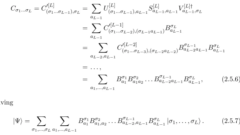
Cσ1...σL =

X

a1,...,aL−1

Aσ1

a1A

σ2

a1a2. . . A

σL−1

aL−2aL−1A

σL

aL−1. (2.5.3)

Inserting into eq. (2.2.9) gives

|Ψi= X

σ1,...,σL

X

a1,...,aL−1

Aσ1

a1A

σ2

a1a2. . . A

σL−1

aL−2aL−1A

σL

aL−1|σ1, . . . , σLi, (2.5.4)

which is the explicit left-canonical form of an MPS. The diagrammatic derivation is given by fig. 2.8. The fact that the A matrices were obtained from the U of an

SVD means that it isleft-normalised, i.e. it satisfies

X

(ai−1,σi)

U_(ai†

−1σi),a0iU(ai−1σi),ai =δa

0

i,ai,

X

(ai−1,σi)

U_a∗0

i,(ai−1σi)U(ai−1σi),ai =δa0i,ai,

X

σi

X

ai−1

A∗_aiσi −1a0iA

σi

(34)

19

Reshape

SVD

S.V Reshape

Reshape

SVD

S.V Reshape

†

[image:34.595.181.451.144.592.2]

Repeat

(35)

(a)

=

(b)

[image:35.595.130.517.323.540.2]

=

Figure 2.9: Diagrammatic representation of (a) left-normalisation given by eq. (2.5.5) and (b) right-normalisation given by eq. (2.5.9).

or diagrammatically in fig. 2.9(a).

Equation (2.5.4) is obtained by starting at site 1 and working towards siteL.

The start point of the derivation does not alter the state, thus an equivalent MPS

can be derived starting fromL and working towards 1,

Cσ1...σL=C

0[L]

(σ1...σL−1),σL=

X

aL−1

U_(σ[L]

1...σL−1),aL−1S

[L]

aL−1,aL−1V

[L]†

aL−1,σL

= X

aL−1

C_(σ0[L−1]

1...σL−2),(σL−1aL−1)B

σL aL−1

= X

aL−2,aL−1

C_(σ0[L−2]

1...σL−3),(σL−2aL−2)B

σL−1

aL−2aL−1B

σL aL−1

= . . . ,

= X

a1,...,aL−1

Bσ1

a1B

σ2

a1a2. . . B

σL−1

aL−2aL−1B

σL

aL−1, (2.5.6)

giving

|Ψi= X

σ1,...,σL

X

a1,...,aL−1

Bσ1

a1B

σ2

a1,a2. . . B

σL−1

aL−2,aL−1B

σL

aL−1|σ1, . . . , σLi. (2.5.7)

This is theright-canonical formof an MPS. TheBmatrices are reshapedV†matrices which satisfy

V†V =11

⇒ (V†)(V†)†=11, (2.5.8)

hence theB matrices are right-normalised

X

σi

X

ai

Bσi_ai₋₁_aiB_a∗σi0

i−1ai

=δ_a0

(36)

Figure 2.10: Diagrammatic representation of an MPS with mixed normali-sation.

The diagrammatic form is given by fig. 2.9(b).

By starting the normalisation process as both ends it is possible to have a

mixed canonicalstate, where the left side is left normalised and the right side is right

normalised. At the point where the two normalisations meet there will be a leftover

matrix of singular values as shown in fig. 2.10. This matrix can be contracted with either neighbouring tensor to make a tensor that does not have either right or left

normalisation. These states will prove useful in calculating expectation values in the

next section. These normalisations do not have any effect on expectation values; as such they are differentgauges.

2.5.2 Overlaps

Orthonormality of the basis vectors and normalisation of the wavefunctions implies that we expecthΨ|Ψi = 1, which is easy to show using the right normalisation of

theA tensors [30]

hΨ|Ψi= X

σ1,...,σL

X

a1,...,aL−1

a01,...,a0L−1

A∗σ1

a0₁ A

∗σ2

a0₁a0₂. . . A

∗σL a0_L−1

×Aσ1

a1A

σ2

a1a2. . . A

σL

aL−1hσ1, . . . , σL|σ1, . . . , σLi

= X

σ2,...,σL

X

a1,...,aL−1

a0₁,...,a0_L−1

" X

σ1

A∗σ1

a0₁ A σ1

a1

#

A∗σ2

a0₁a0₂. . . A

∗σL a0_L₋₁A

σ2

a1a2. . . A

σL aL−1

= X

σ2,...,σL

X

a1,...,aL−1

a0₁,...,a0_L−1

δa0

1a1A

∗σ2

a0₁a0₂. . . A

∗σL a0_L₋₁A

σ2

a1a2. . . A

σL

(37)

=

[image:37.595.212.432.104.408.2]

=

...

=

Figure 2.11: Diagrammatic derivation of the normalisation of a bra-ket as in eq. (2.5.11).

where we have used the conditions on A in eq. (2.5.5). Repeating until the end of

the chain yields the result

hΨ|Ψi= X

σ3,...,σL

X

a2,...,aL−1

a0

2,...,a0L−1

" X

σ2

X

a1

A∗σ2

a1a02A

σ2

a1a2

#

A∗σ3

a0

2a03. . . A

∗σL a0

L−1

Aσ3

a2a3. . . A

σL aL−1

= X

σ3,...,σL

X

a2,...,aL−1

a0

2,...,a0L−1

δ_a0

2a2A

∗σ3

a0

2a03. . . A

∗σL a0

L−1

Aσ3

a2a3. . . A

σL aL−1

=. . . ,

=X

σL

X

aL−1

A∗_aLσL₋₁AσL_aL₋₁

(38)

Figure 2.12: Construction of the left block L in derivation (2.5.12) tensor by tensor.

This derivation can be performed very neatly pictorially as in fig. 2.11. A similar derivation gives the same result for right-normalised B matrices. The overlap of

two wavefunctions (hΦ|Ψi) cannot make use of this convenient normalisation, so it

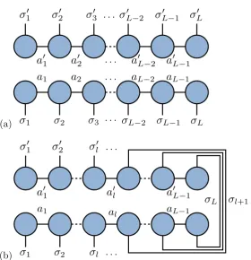
is necessary to contract all of the terms. If each wavefunction is represented by an MPS with a bond dimensionχ this can still be done efficiently

hΦ|Ψi= X

σ1,...,σL

X

a1,...,aL−1

a0₁,...,a0_L₋₁

M0∗σ1

a0

1 M

0∗σ2

a0

1a02. . . M

0∗σL a0

L−1

×Mσ1

a1M

σ2

a1a2. . . M

σL

aL−1hσ1, . . . , σL|σ1, . . . , σLi

= X

σ2,...,σL

X

a1,...,aL−1

a0₁,...,a0_L₋₁

L[1]_a

1a01M

0∗σ2

a0

1a02. . . M

0∗σL a0

L−1M

σ2

a1a2. . . M

σL aL−1

=. . .

= X

σi,...,σL

X

ai−1,...,aL−1

a0_i₋₁...,a0_L₋₁

L[L_ai−1] −1a0i−1M

0∗σi a0

i−1a0i. . . M

0∗σL a0

L−1

M_aiσi₋₁_ai. . . MσL aL−1

=. . . , (2.5.12)

where the M are the MPS tensors for |Ψi and M0∗ are the tensors for hΦ|. The calculation is performed one tensor at a time form left to right, grouping the

con-tracted tensors into ablock L. Figure 2.12 shows the contraction of one site into the

(39)

(a)

[image:39.595.203.484.100.391.2]

(b)

Figure 2.13: (a) MPS density operator ˆρ of eq. (2.5.14) and (b) reduced density operator ˆρA of eq. (2.5.16), where sitesl+ 1 to Lhave been traced

over.

2.5.3 The Density Operator

The density operator for a wavefunction|Ψi is defined as

ˆ

ρ=|Ψi hΨ|. (2.5.13)

For an MPS this takes the form [30]

ˆ

ρ= X

σ1,...,σL

σ01,...,σ0L

X

a1,...,aL

a01,...,a0L

Mσ1

a1 . . . M

σL aL−1M

∗σ0₁ a01 . . . M

∗σ_L0 a0_L−1

|σ1, . . . , σLi hσ01, . . . , σ

0

L|, (2.5.14)

or diagrammatically as in fig. 2.13(a). Like the singular values of an SVD, the

density operator contains the entanglement information of the state. Reduced density operators are calculated by tracing over the degrees of freedom of the system. Most

(40)

reduced density matrices are then

ˆ

ρA= TrB|Ψi hΨ| , ρˆB = TrA|Ψi hΨ|. (2.5.15)

ˆ

ρA can be expressed in MPS form as

ˆ ρA=

X

σ1,...,σL

σ₁0,...,σ_l0

X

a1,...,aL

a0₁,...,a0_L

Mσ1

a1 . . . M

σl al−1alM

σl+1

alal+1. . . M

σL

aL−1 (2.5.16)

×M∗σ 0

1

a0₁ . . . M

∗σ0_l a0_l₋₁a0_lM

∗σl+1

a0_la0_l₊₁. . . M

∗σL

a0_L₋₁|σ1, . . . , σli hσ

0

1, . . . , σ

0

l|,

which is shown in fig. 2.13(b). The contracted tensors of the B block form the

reduced density matrix ρA

ρA=

X

σl+1,...,σL

X

al+1,...,aL−1

Mσl+1

alal+1. . . M

σL aL−1M

∗σl+1

a0_la0_l₊₁. . . M

∗σL a0_L−1

. (2.5.17)

The reduced density matrix for regionB (ρB) can be made using the same argument

but it is the left hand sites that are contracted.

Like the SVD in eq. (2.4.4), the reduced density matrices can be used to

calculate the von Neumann entropy

SA|B=−TrρAlog2ρA=−TrρBlog2ρB. (2.5.18)

The entanglement entropy is the same whether calculated usingρA orρB as it is a

measure of how entangled block A is to B. It is worth noting that to take the log of a matrix it is necessary to diagonalise it and can therefore be computationally

expensive. When the MPS is in a mixed state with the left region left normalised

and the right region right normalised the calculation of entanglement entropy is greatly simplified,ρA of eq. (2.5.17) becomes

ρA=

X

σl+1,...,σL

X

al+1,...,aL−1

SalalB σl+1

alal+1. . . B

σL aL−1Sa0la

0

lB

∗σl+1

a0

la0l+1. . . B

∗σL a0

L−1

=X

al

SalalSa∗0

lal =SS

†_. _(2.5.19)

Similarly ρB = S†S. As S is real and diagonal, ρA =ρB =S2. Thus eq. (2.5.18)

becomes equal to (2.4.4) with the eigenvalues of the reduced density matrix equal

(41)

Figure 2.14: Expectation value for a single site operator.

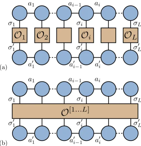
2.5.4 Expectation Values

The expectation value of a local operatorO[i] _{can be calculated in a highly efficient}

manner due to the normalisation of the MPS, where the operator is defined as

O[i]= X

σi,σ0_i

Oσi,σ0i|_σ_ii h_σ0

i|, (2.5.20)

and implicitly acts with an identity on the rest of the sites. An example of such an

operator issz_i, giving the expectation value for the z-component of the spin for site i. If the MPS bra and ket are gauged such that all sites to the left of the operator

are left normalised and all to the right are right normalised, the calculation of the

expectation value is almost trivial, i.e.

hΨ|O[i]_|_Ψ_i₌ X

σ1,...,σL

X

a1,...,aL−1

a0

1,...,a0L−1

A∗σ1

a0

1 . . . A

∗σi−1

a0

i−2a

0

i−1

M∗σ 0

i a0

i−1a

0

i

B∗σi+1

a0

ia

0

i+1

. . . B_a∗0σL

L−1

×Oσiσi0Aσ1 a1. . . A

σi−1

ai−2ai−1M

σi ai−1aiB

σi+1

aiai+1. . . B

σL aL−1

× hσ1. . . σi−1|σ1. . . σi−1i hσi0|σ

0

ii hσi|σii hσi+1. . . σL|σi+1. . . σLi

=X

σiσ0_i

X

ai−1ai

M_ai∗σ₋0₁_aiOσiσ0i_Mσi

ai−1ai, (2.5.21)

where the normalisation of the MPS was used to set the sites to the left and right of

the operator equal to the identity. The diagrammatic representation is given in fig. 2.14. In a similar way to fig. 2.12 it can be shown that (2.5.21) can be performed

inO(χ2d).

(42)

two-(a)

[image:42.595.198.442.106.359.2]

(b)

Figure 2.15: Expectation value for (a) a single site operator acting on all sites and (b) a general operator acting on all sites.

point correlation functions or the totalsz taking the form

hΨ| O[1]_{. . .}_O[L]_|_Ψ_i₌ X

σ1,...σL

σ0

1,...,σL0

X

a1,...,aL−1

a0

1,...,a0L−1

M∗σ 0

1

a01 . . . M

∗σ_L0 a0_L−1

Oσ1σ10 _{. . . O}σLσ0LMσ1. . . Mσ

0

L,

(2.5.22)

or diagrammatically as shown by fig. 2.15(a). Gauging the MPS to a mixed canonical form will provide a simplification to the contraction if there are not operators acting

on the edge sites. In eq. (2.5.22) there is no such simplification as all sites are acted

on by operators, so is calculated inO(Lχ3d). The most general form of expectation value is where the operator is not local and represented by a 2L index tensor,

hΨ| O[1...L]|Ψi= X

σ1,...σL

σ₁0,...,σ_L0

X

a1,...,aL−1

a0₁,...,a0_L₋₁

M∗σ 0

1

a0

1 . . . M

∗σ0

L a0

L−1O

σ1σ10...σLσ0L_Mσ1_{. . . M}σL0_, _(2.5.23)

given by fig. 2.15(b). An example of an operator that takes this form is the Hamil-tonian. Unlike the local operators, contracting full tensor operators means having

(43)

2.6 Matrix Product Operators

The computational cost of storage and manipulation of general tensor operators

scales exponentially with system size as discussed in the previous section. The idea of a matrix product operator (MPO) [30, 46, 47] is to use the ideas of MPSs

to transform the tensor operators into a form that can potentially be contracted

efficiently. A general operator can be written as

O= X

σ1,...σL

σ0

1,...,σ0L

Oσ1σ10...σLσL0 |σ₁. . . σ_Li hσ0

1. . . σL0|. (2.6.1)

This can be decomposed using SVDs in the same way as the MPS derivation for (2.5.4). Proceeding as before with O0 being the matrix resulting from a reshaping of tensorO, we have

Oσ1σ01...σLσ

0

L ₌_O0

σ1σ10,(σ2σ02...σLσ0L)=

X

b1

U_σ[1]

1σ0₁,b1S

[1] b1,b1V

[1]†

b1,(σ2σ0₂...σLσ0_L)

=X

b1

Wσ1σ10

b1 O

0

(σ2σ20,b1),(σ3σ03...σLσ0L)

= X

b1,b2

Wσ1σ10

b1 W

σ2σ02

b1b2 O

0

(σ3σ03,b2),(σ4σ04...σLσL0)

= X

b1,...,bL−1

Wσ1σ01

b1 W

σ2σ20

b1b2 . . . W

σL−1σL0−1

bL−2bL−1 W

σLσ_L0 bL−1

(2.6.2)

The standard form for an MPO is therefore

O= X

σ1,...σL

σ₁0,...,σ_L0

X

b1,...,bL−1

Wσ1σ 0

1

b1 W

σ2σ20

b1b2 . . . W

σL−1σ0L−1

bL−2bL−1 W

σLσ0

L

bL−1 |σ1. . . σLi hσ

0

1. . . σ

0

L|.

(2.6.3)

As usual this derivation can be performed pictorially as in fig. 2.16.

The expectation value hΨ|O|Ψi is found by contracting the MPO with an MPS bra and ket

hΨ|O|Ψi= X

σ1,...,σL

σ₁0,...,σ_L0

X

a1,...,aL

a0₁,...,a0_L

X

b1,...,bL

M∗σ 0

1

a0₁ W σ1σ10

b1 M

σ1

a1M

∗σ02

a0₁a0₂W σ2σ20

b1b2 M

σ2

a1a2×. . .

· · · ×M∗σ 0

L−1

a0_L₋₂a0_L₋₁W

σL−1σL0−1

bL−2bL−1 M

σL−1

aL−2aL−1M

∗σ0_L a0_L₋₁W

σLσ0_L bL−1 M

σL

aL−1. (2.6.4)

(44)

29

S.V Reshape Reshape

SVD

S.V Reshape

Reshape

SVD

†

Repeat

σ'

₁

[image:44.595.163.464.100.702.2]

(45)

Figure 2.17: Diagrammatic form of the expectation value as given by eq. (2.6.4). As usual the circles are MPS tensors and the squares MPO tensors.

the indices explicitly written the expression is rather opaque yet the diagram in fig.

2.17 is easy to understand. Many operators have an MPO representation that has a constant MPObond dimension DW, that is the indices bi have a constant

num-ber of elements. Most noticeably many common Hamiltonians have this property,

for example the Heisenberg and Hubbard models, meaning that calculating energy expectation values becomes efficient taking O(Lχ3DWd).

2.6.1 Explicit form of Matrix Product Operators

Many of the most common lattice Hamiltonians can be written as an MPO with a constant bond dimension DW, so it is useful to understand how these explicit

MPOs are created and manipulated. For more complicated MPOs it is helpful to

use graphical representations. Throughout this sectionmatrix product diagrams will be used but so-calledfinite weight automata are also common [29]. Matrix product

diagrams consist of two columns of points representing the first and second indices of

a matrix, then a labelled arrow connecting a point of the first column to one on the second column is the element in the matrix for those indices. Matrix multiplication

is then simply two of these placed end on end and the matrix elements are the sum

of all the paths that connect the appropriate indices (see fig. 2.18 for an example). The most simple one dimensional nearest-neighbour Hamiltonian with OBCs

takes the form

H=

L−1

X

i=1

(46)

When written explicitly in terms of tensors this is [36]

Hσ1σ10...σLσ

0

L ₌_Aσ1σ

0

1

1 ⊗A

σ2σ02

2 ⊗11σ3σ

0

3 ⊗ · · · ⊗₁₁σiσ

0

i⊗ · · · ⊗₁₁σLσ

0

L

+11σ1σ01 ⊗_Aσ2σ

0

2

2 ⊗A

σ3σ03

3 ⊗ · · · ⊗11σiσ

0

i ⊗ · · · ⊗₁₁σLσ

0

L₊_{. . .}

· · ·+11σ1σ01⊗ · · · ⊗_Aσiσ

0

i

i ⊗A

σi+1σi0+1

i+1 ⊗ · · · ⊗11

σLσ0

L₊_{. . .}

· · ·+11σ1σ0₁_{⊗ · · · ⊗}₁₁σiσ_i0_{⊗ · · · ⊗}_AσL−1σ

0

L−1

L−1 ⊗A

σLσ_L0

L , (2.6.6)

which can be written as an MPO with tensors

W[1]σ1σ 0

i

1b1 =

11σ1σ01 Aσ1σ

0 1 1 0 , (2.6.7) W[i]σiσ 0 i bi−1bi =



  

11σiσ0i Aσiσ

0

i

i 0

0 0 Aσiσ

0

i i

0 0 11σiσ0i



  

, (2.6.8)

W[L]σLσ 0

L bL−11 =

   0 AσLσ 0 L L

11σLσ0L





. (2.6.9)

The matrix product diagrammatic form of eq. (2.6.8) is shown in fig. 2.18(b). The

first and last sites are special cases, they are the first row and last column of the gen-eral case, respectively. These have the diagrammatic form shown in fig. 2.18(a) and

2.18(c), respectively. The product of multiple matrices is represented by

concate-nating multiple of these diagrams as shown in fig. 2.18(d). The resulting operator is the sum of the possible paths across the diagram where the binary operator between

theAi is a tensor product. This gives the explicit form of eq. 2.6.6 as desired.

On-site terms are simple to include in the MPO and have a clear representa-tion in the diagram. They take the top right element of the MPO and connect the

top to the bottom of the diagram directly on that site. An example of a Hamiltonian

with on-site and nearest neighbour terms is

H=

L−1

X

i=1

AiAi+1+ L

X

i=1

Tensor networks and geometry for the modelling of disordered quantum many body systems

University of Warwick institutional repository:

http://go.warwick.ac.uk/wrap

A Thesis Submitted for the Degree of PhD at the University of Warwick

http://go.warwick.ac.uk/wrap/70003

This thesis is made available online and is protected by original copyright.

Please scroll down to view the document itself.

Tensor Networks and Geometry for the Modelling

of Disordered Quantum Many-Body Systems

Andrew M Goldsborough

Physics

Contents

List of Figures

Acknowledgments

Declarations

Abstract

Abbreviations

Chapter 1

Introduction

Chapter 2

Matrix Product States and the

Density Matrix Renormalisation

Group

2.1

White’s Density Matrix Renormalisation Group

Superblock

L R

L

R

L

R

2.2

Introduction to Matrix Product States

2.3

Diagrammatic Notation

=

=

=

2.4

Fundamental Details

1

-8

-1

-2

-3

-4

-7

-6

-5

1

-8

-1

-2

-3

-4

-7

-6

-5

6

5

3

4

7

2

1

8

8

2

3

5

1

4

7

6

2.5

Matrix Product States

=

=

=

=