Kent Academic Repository
Full text document (pdf)
Copyright & reuse
Content in the Kent Academic Repository is made available for research purposes. Unless otherwise stated all content is protected by copyright and in the absence of an open licence (eg Creative Commons), permissions for further reuse of content should be sought from the publisher, author or other copyright holder.
Versions of research
The version in the Kent Academic Repository may differ from the final published version.
Users are advised to check http://kar.kent.ac.uk for the status of the paper. Users should always cite the published version of record.
Enquiries
For any further enquiries regarding the licence status of this document, please contact:
If you believe this document infringes copyright then please contact the KAR admin team with the take-down information provided at http://kar.kent.ac.uk/contact.html
Citation for published version
Zhang, Haomin and McLoughlin, Ian Vince and Song, Yan (2016) Robust sound event recognition
using convolutional neural networks. In: Acoustics, Speech and Signal Processing (ICASSP),
2015 IEEE International Conference, 19-24 April 2015, Brisbane, Australia.
DOI
https://doi.org/10.1109/ICASSP.2015.7178031
Link to record in KAR
http://kar.kent.ac.uk/55020/
Document Version
ROBUST SOUND EVENT RECOGNITION USING CONVOLUTIONAL NEURAL
NETWORKS
Haomin Zhang, Ian McLoughlin, Yan Song
National Engineering Laboratory of Speech and Language Information Processing
The University of Science and Technology of China, Hefei, PRC
ABSTRACT
Traditional sound event recognition methods based on in-formative front end features such as MFCC, with back end sequencing methods such as HMM, tend to perform poorly in the presence of interfering acoustic noise. Since noise corrup-tion may be unavoidable in practical situacorrup-tions, it is important to develop more robust features and classifiers. Recent ad-vances in this field use powerful machine learning techniques with high dimensional input features such as spectrograms or auditory image. These improve robustness largely thanks to the discriminative capabilities of the back end classifiers. We extend this further by proposing novel features derived from spectrogram energy triggering, allied with the powerful classification capabilities of a convolutional neural network (CNN). The proposed method demonstrates excellent per-formance under noise-corrupted conditions when compared against state-of-the-art approaches on standard evaluation tasks. To the author’s knowledge this in the first application of CNN in this field.
Index Terms— Machine hearing, auditory event detec-tion, convolutional neural networks
1. INTRODUCTION
Sound event classification is a developing research field which has traditionally benefitted from advances in more mature research in related areas, such as automatic speech recognition (ASR). Detecting sound events in noise is poten-tially very useful in daily life, such as in allowing a computer to hear and eventually understanding environmental sounds like a human, and from this to infer what is happening in the environment. This technology has implications for improv-ing ASR in many noisy real world scenarios, in security and healthcare monitoring, in intelligent building or city manage-ment, and in environmental analysis [1].
Unlike in spoken language, sound events are more ran-dom, both periodic and aperiodic, with less well defined oc-currence patterns. Sound events also exhibit much wider fre-quency and amplitude ranges, since they are not constrained by production from the human vocal apparatus [2]. These
factors make the task of sound event detection and recogni-tion inherently more difficult than ASR. In fact, ASR-inspired techniques such as MFCC, PLP, ZCR, LSPs [3] have featured prominently in the field [4, 5, 6]. However state-of-the-art ro-bust performance has been achieved only when using higher dimensionality representations such as auditory images [7], spectrogram image features [8] and spectrogram-derived sub-band power distribution [9]. Feature vectors derived from these representations are used in conjunction with machine learning techniques including SVM [10],kNN [9], PAMIR [7] and so on. The objective of these systems is for powerful machine learning capabilities to infer discriminative relation-ships from less refined but higher dimensionality input fea-tures. A baseline comparison of many techniques on standard evaluation tasks, has been performed recently by Dennis [9].
It is notable that, for the robust task (i.e. recognition of sounds in noise), the best performing input features are in fact images [11]. This provides support for adopting machine learning algorithms from the image processing domain. This was the stated reason for adoption of PAMIR with stabilised auditory images (SAI) in [12]. Similarly, the current paper proposes the use of convolutional neural networks (CNN) with a novel spectrogram image feature (SIF), based upon the observation that CNN-based techniques have recently performed well in related image processing tasks [13, 14]. In particular, the fact that general sounds are not precisely lo-calised in the time-frequency spectrogram, but may preserve strong local relationships, means that the global convolution and subsampling approach inherent to the CNN has advan-tages. Therefore, this paper develops and evaluates a novel CNN back-end classifier and SIF feature extraction front-end.
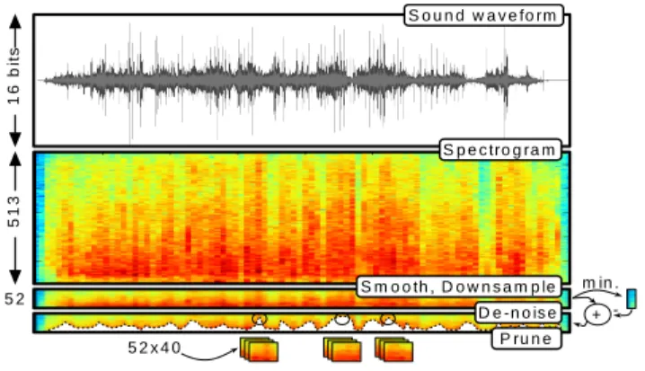
2. IMAGE FEATURE BASED ON SPECTROGRAM This section will detail the formation of SIF vectors from a spectrogram of a sampled sound. Firstly, a spectrogram is generated by stacking fast Fourier transform (FFT) magni-tudes from the original sound’s highly overlapped analysis windows. Given lengthNanalysis frames(n)and Hamming windoww(n), the short time spectral representation of thelth framef(l, k)is obtained,f or k= 0. . .⌊N/2⌋as follows:
Fig. 1. Block diagram of the image feature extraction process. f(l, k) = N−1 X n=0 s(n).w(n).e−j2πnk/N (1) This yields spectrogram image f(l, k) which is then smoothed in frequency using a window of lengthW;
f(l, k) =
W−1 X
i=0
f(l, k+i)/W (2) before being down sampled to a frequency resolution ofB
points by averaging. In fact, preliminary results indicate that further image smoothing, using a simple two element win-dow in the frequency domain, improves results in noisy con-ditions by up to 1% (we will therefore report results both with and without this step). The resulting down sampled and smoothed spectrogram,fb(l, b), is then de-noised by subtract-ing the value of the minimum frequency component found occurring in any frame across the input array:
fdn(l, b) =fb(l, b)−min
l {fb(l, b)} f or b= 1. . . B (3) Finally, per frame time-domain energy,e(l), is computed:
e(l) =
B
X
b=1
fdn(l, b) (4) The three maximum energy indicesJj(j = 1. . .3)are found and used to prune the entire image arrayfdn(l, b)by discard-ing all but the immediate context of the six frames around those energy peaks. This process will therefore yield 18 sep-arate features, SIF, each of which is an L×B dimension
down-sampled, de-noised image, irrespective of the length of the original sound array:
SIF=fdn{κ− ⌊L/2⌋:κ−1 +⌊L/2⌋,1 :B} (5)
whereκ= Jj−2 : Jj + 3 f or j = 1. . .3. The entire feature extraction process flow is illustrated in Fig. 1, from
top to bottom, showing an input sound waveform, forming the overlapped spectrogram, smoothing, down-sampling and de-noising followed by computation of frame-by-frame energy and subsequent pruning. The spectrogram is shown here in colour purely for purposes of illustration.
Note that the authors have investigated a number of alter-native pruning methods which are not detailed here for rea-sons of lack of space. The use of the entire un-pruned stack of down-sampled images for classification was found to be not viable since it takes much longer to train the CNN, which is then much more difficult to achieve convergence. It is not the intention of the authors to claim that the pruning method is optimal, but simply to demonstrate that it is effective. It con-stitutes the first published application of CNN classification to sound event recognition.
3. CNN FOR SOUND EVENT RECOGNITION CNNs are a class of multi-layer neural networks which tain convolution layers, subsampling layers and fully con-nected layers. While the network complexity is high due to the large amount of connectivity, the use of shared weights within layers assists in reducing the number of parameters that need to be trained. However, CNNs share the need, with deep neural networks (DNN), for large amounts of training data. In general, for a convolutional layerl−1, we form layer output maps from
xlj=f(X i∈Mj xl−1 i ∗k l ij+blj), (6) wherexl
jis thejth output map,x l−1
i is theith input map,
klij denotes the kernel that is applied, and Mj represents a
selection of input maps [15]. The subsampling layer is sim-pler,xlj=f(βjldown(xl−1i ) +blj)withdown(.)representing
sub-sampling andβandbare biases [15].
The fully connected output layer is effectively a dual layer multi-layer perceptron (MLP) network, with input layer size depending upon the total number of nodes in the final CNN subsampling layer, but otherwise formed as a typical MLP. Like an MLP, the CNN can be learned by gradient descent using the back-propagation algorithm. As mentioned above,
units in the same feature map share the same parameters, so the gradient of a shared weight is simply computed as the sum of the shared parameter gradients.
The CNN is widely used in image processing [13, 14], where it has demonstrated good performance. Similarly, it has been applied to the ASR field [16, 17], and has been shown to achieve better results than traditional networks for many different tasks. A spectrogram is really a special image con-taining different patterns, many of which exhibit local rela-tionships but only weak absolute locality, i.e. a recognisable sound event may appear at different times and in slightly dif-ferent frequency ranges. They thus appear suitable for classi-fication by CNN, particularly since the CNN is insensitive to patterns at different positions in a image (thanks to the con-volution and subsampling steps). Furthermore, sounds events in daily life usually contain more random patterns than those of speech: they can appear more like random pictures, which means that they are potentially even more suitable for CNN classification than is the speech task.
4. EXPERIMENTS AND RESULTS 4.1. The evaluation task
The sound and noise corpora used in this paper are chosen to match those used to evaluate current state-of-the-art SIF-based methods, as defined by Dennis et. al. [18, 9]. 50 sound classes and 80 sound files are selected randomly from the Real Word Computing Partnership (RWCP) Sound Scene Database in Real Acoustic Environments [19]. Four differ-ent environmdiffer-ents of noise are chosen from the NOISEX-92 database, namely “Destroyer Control Room”, “Speech Bab-ble”, “Factory Floor 1” and “Jet Cockpit 1”.
50 of the 80 files in each class are designated to be a train-ing set (total 2500 files), with the rest formtrain-ing the testtrain-ing set (total 1500 files). During testing, randomly-chosen noise is added from random starting points to the sounds at levels of 20, 10 and 0 dB SNR (plus one test with no noise added). However training uses only clean sounds. The mismatched noise conditions make the task more challenging, but are ar-guably more similar to the situation in reality.
At a 16kHz sample rate, we choose an FFT analysis window length of 1024, which means one frame lasts for
1024/16kHz= 64ms. While speech may be considered pseudo-stationary for around 20ms [2], general environmen-tal sounds are more agile, so we use highly overlapped anal-ysis windows spaced 64 samples apart. This time difference between two frames in the spectrogram array is therefore only 64/16kHz= 4ms, allowing important instantaneous information to be captured.
A typical CNN structure form is chosen to match those used by other authors in the ASR domain. This comprises two convolutional layers with outputmaps of size 6 and 12, a convolution kernel size of5×5and a subsampling kernel size
Table 1. Accuracy (%) against SIF time span.
L clean 20dB 10dB 0dB mean 16 87.40 87.13 85.33 75.67 83.88 20 90.93 90.80 89.13 76.73 86.90 24 93.87 93.93 92.07 79.67 89.89 28 93.60 93.53 91.53 77.40 89.02 32 93.33 93.40 91.67 75.60 88.50 36 93.93 94.27 93.00 77.47 89.67 40 94.40 94.27 92.67 75.13 89.12 44 93.80 93.80 91.00 70.33 87.23 48 64.20 64.00 62.87 49.73 60.20 of2×2. The CNN toolbox [20] is used for all experiments. 4.2. Results and discussion
While the CNN classifier and the input feature representation both involve many parameters which could be individually tuned to improve performance, the following subsections in-vestigate only the effect of different frequency and time res-olutions in the input SIF, the effect of smoothing, and use of Mel-filterbanks to form the CNN input feature. Each test re-quired the creation of a custom-sized CNN which were, apart from the feature under test, identical in other aspects.
4.2.1. The effect of SIF time-span on performance
The number of frames in a feature defines how much time one SIF spans. Since the test data set includes a range of sounds from very short to very long duration, it is not immediately clear what is the optimal time span. We therefore investigate full performance (i.e. in both clean and noisy conditions) with the number of frames in the SIF (L) set from 16 to 48. Re-sults are shown in Table 1, where the frequency resolution is maintained at 24. We can see that performance first rises withL, then drops as it becomes too big, and within the cen-tral region of the table, the performance is relatively flat. We will therefore set the baselineL= 40for future experiments. This value appears to be long enough to contain the necessary timespan, but short enough to maintain sufficient time reso-lution. It yields highest accuracy in clean conditions and yet still maintains good accuracy in noisy conditions.
4.2.2. The effect of frequency resolution on performance
The frequency solution defines how many frequency bands there are in an image feature. We begin by setting the number of frames in the SIF to 40. Then we compute performance as the frequency resolution,B, is swept from 48 to 68 in steps of 4. The results are shown in Table 2. It is clear that best overall performance – in both clean and noisy conditions – is achieved whenB= 52.
Therefore,52×40seems to be a suitable SIF dimension-ality for the given experimental conditions, dataset and
clas-Table 2. Accuracy (%) against frequency resolution. B clean 20dB 10dB 0dB mean 48 96.60 96.27 93.87 79.13 91.47 52 97.33 97.40 95.67 83.07 93.37 56 96.73 96.53 94.27 81.47 92.25 60 97.27 97.07 93.93 79.73 92.00 64 97.27 97.13 94.47 80.13 92.25 68 96.93 97.00 94.27 78.87 91.77
sifier method. All sizes and dimensions of the final CNN and feature extractor were labelled clearly in Figs. 1 & 2.
4.2.3. Comparison with other system
Since we adopt a standard sound recognition task, database and evaluation criteria, it is possible to compare the proposed approach directly with existing state-of-the-art methods. The top part of Table 3 therefore lists a number of results from Dennis [18], with “Dennis SIF” reporting the accuracy that he achieved with a simpler spectrogram image feature and an SVM classifier. The lower part of the table compares our own systems, described as follows:
SIF-CNNis the baseline CNN outlined above. Perfor-mance is extremely good overall, at 93% mean accuracy. While performance with clean sounds is slightly worse than some of the traditional approaches, this is more than com-pensated for by an extremely good 83% accuracy in 0dB SNR conditions. SIF-IS-CNN is identical to the baseline CNN except for a 2-bin frequency domain smoothing ap-plied to the spectrogram prior to de-noising. It is the highest performing system overall, especially for noisy conditions. Further experiments are currently being undertaken to de-termine whether this improvement is due to the smoothing of the de-noising vector or to smoothing of the spectrogram image itself. SIF-IS-DNNimplements a 4-layer DNN using the same input features and number of classes as the CNN system. While there is no guarantee that the optimal dimen-sion of internal layers for the DNN should match that of the CNN, it is at least an indication of DNN performance using the given feature and similar computational load. In fact the performance of this is better than all results reported prior to this paper, apart from the final SIF in [18] and the DNN system in [11].
MelFb-CNNuses the same setup as the SIF-CNN, but in-stead of smoothing the spectrogram image over a window of size W, a standard Mel-filterbank analysis is applied with the motivation that this has shown benefit for similar ASR tasks. Clearly the spectral content of the sounds analysed in this paper differs from that of speech, resulting in a slight performance degradation overall. However it is interesting that the performance in clean and 20dB SNR conditions is actually slightly improved by the use of the Mel-filterbank.
The final results, particularly for SIF-IS-CNN, confirm
Table 3. Classification accuracy (%) for various sound event detection methods (italicised systems are from Dennis [18] and McLoughlin et. al. [11]).
System clean 20dB 10dB 0dB mean
MFCC-HMM 99.4 71.9 42.3 15.7 57.4 MFCC-SVM 98.5 28.1 7.0 2.7 34.1 ETSI-AFE 99.1 89.4 71.7 35.4 73.9 MPEG-7 97.9 25.4 8.5 2.8 33.6 Gabor 99.8 41.9 10.8 3.5 39.0 GTCC 99.5 46.6 13.4 3.8 40.8 MP+MFCC 99.4 78.4 45.4 10.5 58.4 Dennis SIF 91.1 91.1 90.7 80.0 88.5 DNN-SIF 96.0 94.4 93.5 85.1 92.3 SIF-CNN 97.33 97.40 95.67 83.07 93.37 SIF-IS-CNN 97.33 97.27 96.20 85.47 94.07 SIF-IS-DNN 86.67 86.40 85.33 73.53 82.98 MelFb-CNN 97.67 97.53 94.67 70.27 90.04
the benefits of a SIF representation, including smoothing and de-noising, on creating a noise-robust sound event detection method. An excellent 85% accuracy is achieved in 0dB SNR, and mean accuracy exceeding 94%.
5. CONCLUSION
The paper has proposed the use of a convolutional neural net-work (CNN) for robust sound event detection, motivated by the inherent image-like nature of the spectrogram representa-tion – and encouraged by recently reported good CNN perfor-mance for similar ASR tasks. A dimension reduction process has been developed to convert the arbitrary length spectro-gram obtained from a sound recording into smoothed and de-noised spectrogram image feature (SIF) blocks of size52×40. Both the frequency domain resolution and the time span of these blocks have been investigated in terms of classification performance using appropriately sized CNNs. Use of a stan-dard evaluation task adopted by other authors has allowed di-rect comparison with other sound event recognition systems, and has revealed that the proposed CNN formulation, using smoothed and de-noised SIF features, is capable of yielding excellent classification accuracy, especially for the challeng-ing 0dB SNR noise condition. To the author’s knowledge, this paper describes the first published application of CNN to this domain, and yields the best accuracy reported to date from spectrogram features.
6. ACKNOWLEDGEMENTS
The authors would like to acknowledge, the following for supporting this work: National Nature Science Foundation of China (grant 61172158), Chinese Universities Scientific Fund (grants no WK2100060008 and WK2100000002).
7. REFERENCES
[1] Richard F. Lyon, “Machine hearing: an emerging field,”
IEEE Signal Processing Magazine, vol. 42, pp. 1414– 1416, 2010.
[2] Ian Vince McLoughlin,Applied Speech and Audio Pro-cessing, Cambridge University Press, 2009.
[3] Ian Vince McLoughlin, “Review: Line spectral pairs,”
Signal processing, vol. 88, no. 3, pp. 448–467, 2008. [4] Axel Plinge, Ren´e Grzeszick, and Gernot A Fink, “A
bag-of-features approach to acoustic event detection,” in
Acoustics, Speech and Signal Processing, 2014. ICASSP 2014 Proceedings. 2014 IEEE International Conference on. IEEE, 2014, pp. 3732–3736.
[5] Michael Casey, “Mpeg-7 sound-recognition tools,”
IEEE Transactions on circuits and Systems for video Technology, vol. 11, no. 6, pp. 737–747, 2001.
[6] Selina Chu, Shrikanth Narayanan, and C-CJ Kuo, “En-vironmental sound recognition with time–frequency au-dio features,”Audio, Speech, and Language Processing, IEEE Transactions on, vol. 17, no. 6, pp. 1142–1158, 2009.
[7] Thomas C Walters, Auditory-based processing of com-munication sounds, Ph.D. thesis, University of Cam-bridge, 2011.
[8] Jonathan Dennis, Huy Dat Tran, and Haizhou Li, “Spec-trogram image feature for sound event classification in mismatched conditions,” Signal Processing Letters, IEEE, vol. 18, no. 2, pp. 130–133, 2011.
[9] Jonathan Dennis, Huy Dat Tran, and Eng Siong Chng, “Image feature representation of the subband power dis-tribution for robust sound event classification,” Audio, Speech, and Language Processing, IEEE Transactions on, vol. 21, no. 2, pp. 367–377, 2013.
[10] Guodong Guo and Stan Z Li, “Content-based audio classification and retrieval by support vector machines,”
Neural Networks, IEEE Transactions on, vol. 14, no. 1, pp. 209–215, 2003.
[11] Ian McLoughlin, Zhang H.-M., Xie Z.-P., Song Y, and Xiao W, “Robust sound event classification using deep neural networks,” Audio, Speech, and Language Pro-cessing, IEEE Transactions on, vol. PP, no. 99, 2015. [12] Richard F Lyon, Jay Ponte, and Gal Chechik, “Sparse
coding of auditory features for machine hearing in in-terference,” in Acoustics, Speech and Signal Process-ing (ICASSP), 2011 IEEE International Conference on. IEEE, 2011, pp. 5876–5879.
[13] Yann LeCun and Yoshua Bengio, “Convolutional net-works for images, speech, and time series,” The hand-book of brain theory and neural networks, vol. 3361, 1995.
[14] Yann LeCun, L´eon Bottou, Yoshua Bengio, and Patrick Haffner, “Gradient-based learning applied to document recognition,” Proceedings of the IEEE, vol. 86, no. 11, pp. 2278–2324, 1998.
[15] Jake Bouvrie, “Notes on convolutional neural net-works,” 2006.
[16] Ossama Abdel-Hamid, Abdel-rahman Mohamed, Hui Jiang, and Gerald Penn, “Applying convolutional neural networks concepts to hybrid nn-hmm model for speech recognition,” inAcoustics, Speech and Signal Process-ing (ICASSP), 2012 IEEE International Conference on. IEEE, 2012, pp. 4277–4280.
[17] Tara N Sainath, Abdel-rahman Mohamed, Brian Kings-bury, and Bhuvana Ramabhadran, “Deep convolutional neural networks for lvcsr,” in Acoustics, Speech and Signal Processing (ICASSP), 2013 IEEE International Conference on. IEEE, 2013, pp. 8614–8618.
[18] Jonathan William Dennis, Sound Event Recognition in Unstructured Environments using Spectrogram Image Processing, Ph.D. thesis, Nanyang Technological Uni-versity, Singapore, 2014.
[19] Satoshi Nakamura, Kazuo Hiyane, Futoshi Asano, Takeshi Yamada, and Takashi Endo, “Data collection in real acoustical environments for sound scene under-standing and hands-free speech recognition,” in EU-ROSPEECH, 1999, pp. 2255–2258.
[20] Rasmus Berg Palm, “Prediction as a candidate for learn-ing deep hierarchical models of data,”Technical Univer-sity of Denmark, Palm, 2012.
![Table 3. Classification accuracy (%) for various sound event detection methods (italicised systems are from Dennis [18]](https://thumb-us.123doks.com/thumbv2/123dok_us/9000950.2797907/5.918.473.835.171.431/classification-accuracy-various-detection-methods-italicised-systems-dennis.webp)
