Simulation Study on the Effects of
Ignoring Clustering in Regression
Analysis
28
thJune 2019
Johanna Thommai
s1793616
Department of Research Methodology, Measurement and Data Analysis (OMD)
First supervisor: prof. dr. ir Jean-Paul Fox
ABSTRACT
In the following, a simulation study was conducted in order to examine the effects of clustering on the precision of the model parameter estimates. One assumes that estimates will appear to be biased when disregarding part of the random effect structure. When taking clustering effects out of the equation more information will be assumed than the data actually contains, which leads to an overstatement of the precision and to false claims about statistical significance. The other way around, an overestimation of the random effect structure will imply non-existing correlations between observations, which leads to an underestimation of the precision. In order to test this assumption, simulated data is used to examine the under- and overestimation of the precisions. Furthermore, we are interested in the bias of standard error estimates of the fixed effects, when mis-specifying the clustering effects. Statistical analysis of p-values and standard errors of the intercepts and fixed effects in the Linear Mixed Effect Model and Linear Model showed that failing to account for clustering effects leads to extreme and biased outcomes which in turn will lead to false conclusions. Moreover, it was found that when dealing with negatively clustered data, ANVOCA, LME and LM falsely proposed that there was no evidence for clustering.
Keywords: Clustering effects, Linear Mixed Models, Model fit, simulation study, random intercept model
1. Introduction
Clustered designs play a major role in educational (Barcikowski, 1981) and clinical and
health research, especially in intervention-related studies, where individuals need to be assigned
or treatment effects (Galbraith, Daniel & Vissel, 2010). As they thereby build the foundation of
the majority of biological research it is of importance that research is conducted with appropriate
statistical methods of analysis in order to produce valid and robust conclusions (Galbraith,
Daniel & Vissel, 2010). A sampling design is regarded as clustered whenever it can be classified
into a number of distinct groups with having more than at least two levels, namely one individual
and one group level (Galbraith et al., 2010). This key feature gives the data the hierarchical, also
called multilevel nature and assumes that within groups have more similarities than between
groups, which implies correlated observations within a group (Galbraith et al., 2010).
When analyzing hierarchical data the intra-class correlation (ICC) coefficient plays a
central role as above described correlation, also called similarity, dependency or
non-independence within a group, is measured by the ICC (Pryseley et al., 2011; Galbraith et al.,
2010; Baldwin, Murray & Shadish, 2005). Hence, the ICC coefficient is the quantitative measure
of variance accounted for by clustering effects. Thus, the greater the ICC rate the stronger is the
design effect due to similarity within groups (Dorman, 2008). The ICC can be both positive and
negative as a common correlation (Kenny & Judd, 1986). According to Pryseley et al. (2011),
negative correlations can be interpreted as negative within-unit correlation suggesting
dissimilarity within the cluster. Further, Pryseley and colleagues (2011) assume that negative
ICC values arise as a result of unstable variance or covariance which in turn is hindering
convergence. This hampering can be decreased by increasing sample and cluster sizes. Hence
they argued that small sample and cluster sizes are a supporting factor of negative ICC.
Moreover, it is suggested that this negative variance component is rather normal for linear
within-group correlation values can arise from compositional or non-random sampling as
dissimilar units might be sampled (Kenny & Judd, 1986; Wang, Yandell & Rutledge, 1992).
Handling clustered data seems to pose an issue on researchers as the methods of handling
clustering are not well developed nor widely understood yet (Galbraith et al., 2010). Thus, when
encountering clusters researchers have assumed that the observations within the data are
independent and thereby ignored the clustering effects and used the individual mean as the unit
of analysis (Galbraith et al., 2010; Barcikowski, 1981). Another approach applied by researchers
is to include the clustering effect as a factor in a regression model. However, this approach fails
to allow for a within-group cluster comparison as ANOVA is only able to represent information
from one treatment group. Therefore, the information is not sufficient to estimate both group and
fixed effects for the clusters (Galbraith et al., 2010). When negative ICC values were obtained,
Wang and colleagues (1991) showed that researchers tend to ignore these values altogether by
either setting the ICC to zero or simply not reporting the obtained values.
However, approaching clustered data in the afore-described manner poses several issues.
Ignoring the clustering effect when conducting analysis is considered incorrect according to
Barcikowski (1981) as it will yield inappropriate outcomes of clustered data since the analysis of
significance is only executed on one level. In other words, when researchers choose one level
over the other they run the risk of either losing statistical power when ignoring the individual
level, or putting the internal validity at stake by running the analysis solely on the individual
level (Barcikowski, 1981). When the clustering level is chosen as the unit of analysis, individual
differences are lost which results in the fact that the effect of individual variability cannot be
determined in a proper way. Moreover, the numbers of clusters are normally small within each
large differences and hence increasing the Type II error rate (Barcikowski, 1981). The more
common way is to analyze for significance only on the individual level and ignoring clustering
effects of the data by using statistical techniques as the linear regression model or fixed effects of
variance models. These models treat all observations as independent from each other and solely
focus on individual differences. However, it is crucial to take into account that by grouping
individuals together, even in randomized samples, individuals are influenced and will influence
each other and thereby creating a so-called class effect (Barcikowski, 1981; Dorman, 2008).
Therefore, individuals who are being observed in clusters require for individual-level analysis to
take this clustering effect into account in order to maintain a nominal Type I error rate for the
fixed effects (Matuschek, Kliegl, Vasishth, Baayen & Bates, 2017). Furthermore, ignoring
clustering effects can lead to over-precise estimates and too extreme p-values as the differences
between clusters are ignored (Lee & Thompson, 2005).
This paper will focus on the latter approach when clustering effects are ignored and
analysis is carried out on the individual level. Therefore, the goal of this study is to investigate
possible consequences when clustering effects are ignored in nested data. More specifically, it is
aimed to examine to what extent bias in the model estimates like standard errors and p-values of
fixed effects and intercepts can occur when ignoring any clustering in the data. Furthermore,
focus will be laid on whether there is a difference in ignoring negative or positive within-cluster
correlations. Lastly, this study is going to test if there is sufficient evidence for clustering effects
2. Methods
2.1 Models
In order to execute the aforementioned research goals of this paper, following models are the focus of this simulation study.
2.1.1 Linear Model (LM)
yij=β0+β1x+εij (1)
where y is the dependent variable for the unit i in cluster j, with i=1,..., n , the x as the independent variable, β0 is the intercept and β1x the slope of the regression line.
2.1.2 Linear Mixed Effects Model (LME)
yij=Xβ+Zu+εij (2a) with β∼N(μ , σ)
(2b)
where y is the outcome variable for the unit i in cluster j, X is the matrix of the predictor variable, β the column vector of the fixed-effects regression coefficients, Z is the design matrix for the random effects with u as the vector and ε is the error term
2.2 Procedure
In this study, a Monte Carlo simulation was conducted. The data were generated under
an LME model, which can generate data with observations in a cluster that are positively
correlated. Data that had negatively correlated observations in a cluster were generated according
to a multivariate model with a covariance matrix displaying the dependence structure in a cluster.
In order to test the research goals, the parameters were re-estimated with lmer which accounts for
positive correlation and with lm in order to compare how the results change when the correlation
in the data was ignored.
2.3 Design
A Monte Carlo simulation study consisting of one condition the strength of cluster
dependence, with a= 20 clusters and n= 5 observations within clusters, running the simulation
with 1000 replications, was executed. As one of the goals was to investigate whether there was a
difference in ignoring positive or negative correlation, the simulation included 15 values of
correlation ranging from -.19 to no correlation (.00) up to a positive correlation with the highest
one being .20. As a large sample and cluster size can adjust and compensate for negative
correlation (Pryseley et al., 2011) a relatively small cluster size was chosen of a= 20.
Furthermore, the study aimed to investigate whether an incorrect random intercepts model had a
negative influence on the other estimates within a statistical model. Therefore, p-values of
intercept and fixed effects were computed within an LME and ANCOVA model in order to
examine any biased pattern in the form of extreme p-values. The same was executed for the
Lastly, the study's goal was to find sufficient evidence for clustering effects. Therefore,
the p-value for testing the significance of clustering under ANVOCA and the ANOVA test under
LME were computed. In order to check whether the LME or LM fits the data best, the Bayesian
Information Criterion (BIC) was computed to choose the best fitting model, where the model
with the smallest BIC value was preferred. Finally, the probability of a within-cluster correlation
being larger than zero was computed for each value of correlation under a multivariate statistical
model, as this multivariate model can include both negative and positive correlations and was
expected to give appropriate results.
3. Results
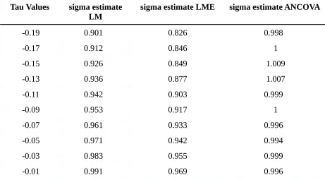
As expected, both LM and LME as models of analysis produced biased estimates of the
measurement error variance (sigma) when true values of correlation were negative. As can be
seen in Table 1, sigma estimates for LME ranged from .826 to .995 and constantly increased with
higher correlation values. It was expected that the LME would yield better results for positive
correlations. LM cannot handle correlations and was expected to produce biased estimates for the
variance in case of correlated outcome data. However, with LM values between .901 and 1.091,
better results were obtained than expected. Moreover, it can be concluded that the residual
variance estimates under LM did not suffice from positive correlations in the data since the
estimated values for the error variance ranged from 1.018 to 1.091 for the highest positive
correlation. In accordance with beforehand made assumptions, the ANCOVA is able to
appropriately estimate the error variance across both negative and positive correlations with
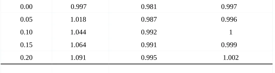
Moreover, as can be seen in Table 2 the analysis results of the slope and intercept
estimates for LM, LME and ANCOVA show that these estimates are affected by neither the
negative nor the positive correlations. The values for the fixed effect (Betaf) were close to the
true value of .1 and imply that the results were not biased. Furthermore, it becomes visible that
the values for all three models of analysis are quite similar when considering the estimates for
the fixed effects, once again confirming that changing the correlation did not have an influence
on the fixed effect estimates.
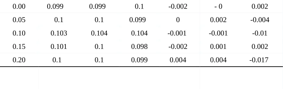
Table 3 displays the p-values of the (Betaf) effect of the predictor variable and intercept
estimates. It can be seen that when testing for this intercept with a true value of 0 as the null
hypothesis the p-values for the intercept for the LM and LME display quite extreme ranges for
the intercept estimates for both negatively and positively correlated data. The highest negative
correlation yields a p-value of .842 and the highest positive correlation displays a value of .497
for the LME and .424 for the LM. From this, it can be inferred that the t-test is not appropriately
measuring statistical significance but is assuming more information than there actually is for the
positively correlated data and underestimates the information for negative correlations. Coming
to the results of the fixed effect, Betaf, it can be seen that both models produce similar values,
namely being around .376 for both negative and positive correlation. Hence, no difference
between the models is to be seen once again which in turn is accounted by the non-differing
means of the fixed effect Betaf. This demonstrates that when the correlation is ignored, statistical
tests of significance will produce biased p-value results.
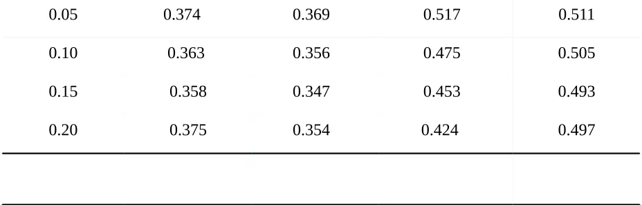
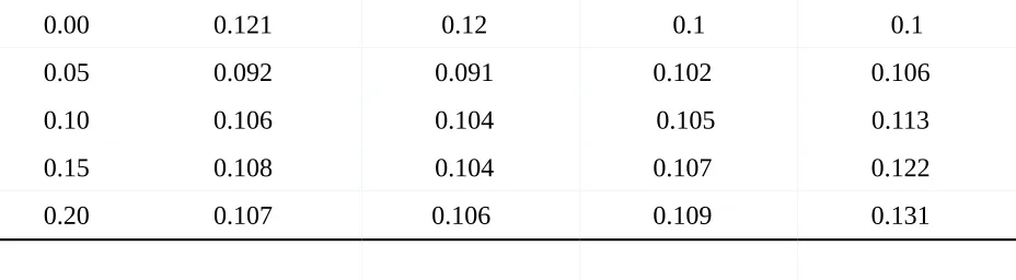
When analyzing the values of the standard error of the fixed effect in LM and LME one
aspect strikes odd. When looking at Table 4 one sees that the measurement of standard errors for
as a difference was expected. One would expect that the LME fits better for the positive
correlations than LM. The results suggest, however, that there is no impact on the estimations of
the slope with varying positive correlations. Further, the standard errors of the intercept estimates
were computed and compared for LM and LME. Here, similar results can be observed. Both
models produced similar standard error estimates with values ranging from .091 to 0.109. It can
be seen that standard error estimates for both models become larger as true values of correlation
increase which is opposed to the expected assumption.
Another goal of this study was to investigate whether we can find sufficient evidence for
clustering effects. In comparison to each other, the LM is always chosen over the LME model
which suggests that the BIC is not a powerful method for detecting evidence of a positive
clustering in the data. The LM does account for any correlation in the data, yet the BIC suggests
that the LM is to be preferred and that there is, therefore, no evidence for clustering effects.
Concluding from that it means that the BIC is not measuring sufficiently the support for
clustering in the data. When looking at the p-values for ANCOVA and the LME it becomes clear
that these two methods as well fail to identify any clustering effects and falsely claim that there is
no sufficient evidence when using a significance level of .05. The p-values for the negative
correlation are exactly 1.0 in both methods and become increasingly smaller for the positive ones
with .097 for the highest positive correlation in ANCOVA and .209 for the random intercept,
which is low. Lastly, it can be seen that the estimations under the multivariate model, which
incorporates both negative and positive correlation, seem to be sufficient. When considering the
probability that the correlation is positive under the multivariate model, P(tau>0), i.e., the
probability of the correlation being greater than 0, we get a probability of 0 for the negative
than 0, it is not likely to yield larger probabilities. With increasing true values of correlation, the
probability as well rises suggesting that for a correlation of .20 the probability that the correlation
is greater than 0 equals 93.9% (.939) and for no correlation 52.2% (.522). Based on these
findings, it can be concluded that the multivariate model is the sufficient method of analysis in
this comparison that accounts for both negative and positive clustering and yields appropriate
evidence.
4. Discussion
The main purpose of this simulation study was to investigate the effects of clustering in
the data and to examine its impact on the model estimates when correlation is ignored.
Furthermore, it was aimed to test whether there was a difference in ignoring negative or positive
correlation and if there was sufficient evidence for clustering effects. For these goals, a
simulation study was executed in RStudio with focus on standard error and p-value estimates for
the intercept and fixed effect and model comparison in order to investigate clustering effects. The
model comparison shows that leaving out correlation will result in false statistical outcomes as
the BIC always seem to favor the LM model, which does not account for any correlation, as the
preferred method of analysis over the LME. Moreover, ANCOVA and the random intercept of
the LME produced extreme p-values for both negative and positive correlation. The multivariate
model, however, yielded sufficient results and showed proper support for clustering in the data.
Further, results showed that both standard errors and p-values are biased and produce extreme
values with standard errors of the intercept being too low for positive correlations and too high
for negative ones. P-values of the intercept show that the statistical test of significance fails to
with research done in the past. Dorman's (2008) study of clustering effects in classroom
environments illustrated that ignoring even moderate ICC values (i.e., .05 < ρ < .10), will lead to
inflated Type I error rates. Further, the study conducted by Galbraith and colleagues (2010) as
well demonstrate that correlation within clustered data needs to be taken into account in order to
avoid extreme p-values.
When computing p-values and standard error estimates for the fixed effect in LME and
LM it becomes clear that the values do not differ from each other, which was probably caused by
the fact that the groups did not differ for the fixed effect but differed for the intercepts. For future
research, it might be interesting to also use random slopes in order to investigate how clustering
effects influence them. The current study does not take this into account which produced results
that do not differ and thereby suggest no impact as now. However, it is possible that the bias
cancel each other out, which can be an explanation for the values produced in this study.
Another remark for future research is to create more conditions in order to compare
varying cluster and sample sizes, and more fixed effects. That way more insightful information
can be gained .
Taking all of the above-described results into consideration, it can be concluded that
clustering effects do have an important effect on the model parameters and estimations. Leaving
them out will lead to bias, suggesting either statistical significance when there is none or the
other way around. It is thus recommended to choose appropriate statistical models, like the
multivariate model, that can account for both negative and positive correlation and thereby
produces more accurate results. As clustered data plays a major role in biological, health and
educational research, it is important to appropriately account for clustering effects as otherwise
REFERENCES
Barcikowski, R. (1981). Statistical Power with Group Mean as the Unit of Analysis. Journal Of
Educational Statistics, 6(3), 267. doi: 10.2307/1164877
Baldwin, S., Murray, D., & Shadish, W. (2005). Empirically supported treatments or type I
errors? Problems with the analysis of data from group-administered treatments. Journal
Of Consulting And Clinical Psychology, 73(5), 924-935. doi:
10.1037/0022-006x.73.5.924
Dorman, J. (2008). The effect of clustering on statistical tests: an illustration using classroom
environment data. Educational Psychology, 28(5), 583-595. doi:
10.1080/01443410801954201
Fox, J. (2008). Applied regression analysis and generalized linear models (2nd ed.). Thousand
Galbraith, S., Daniel, J., & Vissel, B. (2010). A Study of Clustered Data and Approaches to Its
Analysis. Journal Of Neuroscience, 30(32), 10601-10608. doi:
10.1523/jneurosci.0362-10.2010
Kenny, D., & Judd, C. (1986). Consequences of violating the independence assumption in
analysis of variance. Psychological Bulletin, 99(3), 422-431. doi:
10.1037//0033-2909.99.3.422
Lee, K., & Thompson, S. (2005). The use of random effects models to allow for clustering in
individually randomized trials. Clinical Trials: Journal Of The Society For Clinical
Trials, 2(2), 163-173. doi: 10.1191/1740774505cn082oa
Matuschek, H., Kliegl, R., Vasishth, S., Baayen, H., & Bates, D. (2017). Balancing Type I error
and power in linear mixed models. Journal Of Memory And Language, 94, 305-315. doi:
10.1016/j.jml.2017.01.001
Pryseley, A., Tchonlafi, C., Verbeke, G., & Molenberghs, G. (2011). Estimating negative variance
components from Gaussian and non-Gaussian data: A mixed models approach.
Computational Statistics & Data Analysis, 55(2), 1071-1085. doi:
10.1016/j.csda.2010.09.002
Wang, C., Yandell, B., & Rutledge, J. (1992). The dilemma of negative analysis of variance
estimators of intraclass correlation. Theoretical And Applied Genetics, 85(1), 79-88. doi:
APPENDIX A
Table 1
Sigma estimates
Tau Values sigma estimate
LM sigma estimate LME sigma estimate ANCOVA
-0.19 0.9010 0.8260 0.9980
-0.17 0.9120 0.846 1
-0.15 0.9260 0.849 1.009
-0.13 0.9360 0.877 1.007
-0.11 0.9420 0.903 0.9990
-0.09 0.9530 0.917 1
-0.07 0.9610 0.933 0.9960
-0.05 0.9710 0.942 0.9940
-0.03 0.9830 0.955 0.9990
0.00 0.9970 0.981 0.9970
0.05 1.018 0.987 0.9960
0.10 1.044 0.992 1
0.15 1.064 0.991 0.9990
[image:16.612.92.559.72.197.2]0.20 1.091 0.995 1.002
Table 2
Beta F and Intercept estimates
Tau Values
Beta F LM Beta F LME
Beta F ANCOVA
Intercept LM
Intercept LME
Intercept ANCOVA
-0.19 0.0960 0.096 0.0950 - 01 - 01 -0.0020
-0.17 0.102 0.1020 0.101 0.0010 0.0020 0.0070
-0.15 0.103 0.103 0.1040 0.0010 0.0010 0.0040
-0.13 0.097 0 0.0970 0.097 - 0.0021 - 01 0.0050
-0.11 0.098 0 0.0980 0.098 -0.0030 0.0010 0.0030
-0.09 0.102 0.1020 0.102 -0.0030 0.0050 0.0010
-0.07 0.099 0 0.0990 0.1 0.0010 -0.0030 -0.025 0
-0.05 0.102 0 0.102 0.103 -0.0020 0.0010 0
-0.03 0.098 0 0.0980 0.0980 -0.000 0.0060 -0.015 0
0.00 0.09900 0.0990 0.1 -0.0020 - 01 0.0020
0.05 0.1 0.1 0.0990 01 0.0020 -0.0040
0.10 0.103 0.104 0.104 -0.001 0 -0.0010 -0.010
0.15 0.101 0.1 0.098 -0.0020 0.0010 0.0020
[image:17.612.76.537.73.218.2]0.20 0.10 0.1 0.099 0.0040 0.0040 -0.017 0
Table 3
P-Values of Beta F and Intercept estimates
Tau Values Beta F p-value
LM Beta F p- value LME Intercept p-value LM intercept p-value LME
-0.19 0.3760 0.3760 0.8420 0.8420
-0.17 0.37 0.370 0.7440 0.7440
-0.15 0.3660 0.3660 0.6820 0.6820
-0.13 0.3530 0.3530 0.6190 0.6190
-0.11 0.367 0.3720 0.5970 0.5970
-0.09 0.3670 0.3670 0.5850 0.586
-0.07 0.3580 0.3570 0.5460 0.548
-0.05 0.35 0.350 0.53 0.535
-0.03 0.339 0 0.3390 0.5310 0.541
-0.01 0.337 0.3370 0.5220 0.538
0.05 0.374 0 0.3690 0.5170 0.511
0.10 0.363 0.3560 0.4750 0.505
0.15 0.358 0.3470 0.4530 0.493
[image:18.612.92.556.73.221.2]0.20 0.375 0.3540 0.4240 0.497
Table 4
Standard Error of Beta F and Intercept estimates
Tau Values SE Beta F LM SE Beta F LME SE Intercept LM SE Intercept
LME
-0.19 0.0910 0.0910 0.0910 0.0910
-0.17 0.0960 0.0960 0.0920 0.0920
-0.15 0.0970 0.0970 0.0930 0.0930
-0.13 0.0930 0.0930 0.0940 0.0940
-0.11 0.0940 0.0940 0.0970 0.0970
-0.09 0.0960 0.060 0.0960 0.0970
-0.07 0.0970 0.09370 0.0980 0.0990
-0.05 0.1030 0.1030 0.9900 0.1
-0.03 0.090 0.090 0.0980 0.1010
0.00 0.1210 0.120 0.1 0.1
0.05 0.0920 0.0910 0.1020 0.1060
0.10 0.1060 0.1040 0.1050 0.1130
0.15 0.1080 0.1040 0.1070 0.1220
[image:19.612.75.539.72.200.2]0.20 0.1070 0.10600 0.1090 0.1310
Table 5
Evidence for clustering effects
Tau Values
ANCOVA p-value
LME p-value random intercept
BIC LM BIC LME P(tau>0)
-0.19 1.0 1 274.122 278.7915 0
-0.17 1.0 1 276.565 282.3918 0
-0.15 0.9950 1 279.738 282.8716 0
-0.13 0.9730 1 281.829 286.436 0.0060
-0.11 0.9320 1 283.153 287.8727 0.0290
-0.09 0.8630 0.9920 285.38 289.4982 0.0880
-0.07 0.7860 0.9770 287.155 292.5436 0.160
-0.05 0.7030 0.9450 289.117 293.5946 0.2630
-0.03 0.6110 0.8990 291.703 296.1523 0.3640
-0.01 0.5440 0.8340 293.338 298.2549 0.4580
0.00 0.4840 0.7980 294.531 298.7387 0.5220
0.05 0.3060 0.6170 298.667 302.25 0.6960
0.15 0.1370 0.320 307.515 308.7636 0.8860