University of Warwick institutional repository: http://go.warwick.ac.uk/wrap
A Thesis Submitted for the Degree of PhD at the University of Warwick
http://go.warwick.ac.uk/wrap/50023
This thesis is made available online and is protected by original copyright.
Please scroll down to view the document itself.
Library Declaration and Deposit Agreement
1. STUDENT DETAILS
Please complete the following:
Full name: ………. University ID number: ………
2. THESIS DEPOSIT
2.1 I understand that under my registration at the University, I am required to deposit my thesis with the University in BOTH hard copy and in digital format. The digital version should normally be saved as a single pdf file.
2.2 The hard copy will be housed in the University Library. The digital version will be deposited in the University’s Institutional Repository (WRAP). Unless otherwise indicated (see 2.3 below) this will be made openly accessible on the Internet and will be supplied to the British Library to be made available online via its Electronic Theses Online Service (EThOS) service.
[At present, theses submitted for a Master’s degree by Research (MA, MSc, LLM, MS or MMedSci) are not being deposited in WRAP and not being made available via EthOS. This may change in future.]
2.3 In exceptional circumstances, the Chair of the Board of Graduate Studies may grant permission for an embargo to be placed on public access to the hard copy thesis for a limited period. It is also possible to apply separately for an embargo on the digital version. (Further information is available in the Guide to Examinations for Higher Degrees by Research.)
2.4 If you are depositing a thesis for a Master’s degree by Research, please complete section (a) below. For all other research degrees, please complete both sections (a) and (b) below:
(a) Hard Copy
I hereby deposit a hard copy of my thesis in the University Library to be made publicly available to readers (please delete as appropriate) EITHER immediately OR after an embargo period of ………... months/years as agreed by the Chair of the Board of Graduate Studies.
I agree that my thesis may be photocopied. YES / NO (Please delete as appropriate)
(b) Digital Copy
I hereby deposit a digital copy of my thesis to be held in WRAP and made available via EThOS.
Please choose one of the following options:
EITHER My thesis can be made publicly available online. YES / NO(Please delete as appropriate)
OR My thesis can be made publicly available only after…..[date] (Please give date)
YES / NO(Please delete as appropriate)
OR My full thesis cannot be made publicly available online but I am submitting a separately identified additional, abridged version that can be made available online.
YES / NO (Please delete as appropriate)
3. GRANTING OF NON-EXCLUSIVE RIGHTS
Whether I deposit my Work personally or through an assistant or other agent, I agree to the following:
Rights granted to the University of Warwick and the British Library and the user of the thesis through this agreement are non-exclusive. I retain all rights in the thesis in its present version or future versions. I agree that the institutional repository administrators and the British Library or their agents may, without changing content, digitise and migrate the thesis to any medium or format for the purpose of future preservation and accessibility.
4. DECLARATIONS
(a) I DECLARE THAT:
I am the author and owner of the copyright in the thesis and/or I have the authority of the authors and owners of the copyright in the thesis to make this agreement. Reproduction of any part of this thesis for teaching or in academic or other forms of publication is subject to the normal limitations on the use of copyrighted materials and to the proper and full acknowledgement of its source.
The digital version of the thesis I am supplying is the same version as the final, hard-bound copy submitted in completion of my degree, once any minor corrections have been completed.
I have exercised reasonable care to ensure that the thesis is original, and does not to the best of my knowledge break any UK law or other Intellectual Property Right, or contain any confidential material.
I understand that, through the medium of the Internet, files will be available to automated agents, and may be searched and copied by, for example, text mining and plagiarism detection software.
(b) IF I HAVE AGREED (in Section 2 above) TO MAKE MY THESIS PUBLICLY AVAILABLE DIGITALLY, I ALSO DECLARE THAT:
I grant the University of Warwick and the British Library a licence to make available on the Internet the thesis in digitised format through the Institutional Repository and through the British Library via the EThOS service.
If my thesis does include any substantial subsidiary material owned by third-party copyright holders, I have sought and obtained permission to include it in any version of my thesis available in digital format and that this permission encompasses the rights that I have granted to the University of Warwick and to the British Library.
5. LEGAL INFRINGEMENTS
I understand that neither the University of Warwick nor the British Library have any obligation to take legal action on behalf of myself, or other rights holders, in the event of infringement of intellectual property rights, breach of contract or of any other right, in the thesis.
Please sign this agreement and return it to the Graduate School Office when you submit your thesis.
AUTHOR:Steven Gary Parsons DEGREE: Ph.D.
TITLE:Eclipsing white dwarf binaries
DATE OF DEPOSIT: . . . .
I agree that this thesis shall be available in accordance with the regulations governing the University of Warwick theses.
I agree that the summary of this thesis may be submitted for publication. I agree that the thesis may be photocopied (single copies for study purposes only).
Theses with no restriction on photocopying will also be made available to the British Library for microfilming. The British Library may supply copies to individuals or libraries. subject to a statement from them that the copy is supplied for non-publishing purposes. All copies supplied by the British Library will carry the following statement:
“Attention is drawn to the fact that the copyright of this thesis rests with its author. This copy of the thesis has been supplied on the condition that anyone who consults it is understood to recognise that its copyright rests with its author and that no quotation from the thesis and no information derived from it may be published without the author’s written consent.”
AUTHOR’S SIGNATURE: . . . .
USER’S DECLARATION
1. I undertake not to quote or make use of any information from this thesis without making acknowledgement to the author.
2. I further undertake to allow no-one else to use this thesis while it is in my care.
DATE SIGNATURE ADDRESS
Eclipsing white dwarf binaries
by
Steven Gary Parsons
Thesis
Submitted to the University of Warwick for the degree of
Doctor of Philosophy
Department of Physics
Contents
List of Tables v
List of Figures vii
Acknowledgments x
Declarations xi
Abstract xiii
Chapter 1 Introduction 1
1.1 Prelude . . . 1
1.2 Binary star evolution . . . 3
1.2.1 Post common envelope binaries . . . 6
1.2.2 Double white dwarf binaries . . . 7
1.3 Period change mechanisms . . . 8
1.3.1 Gravitational radiation . . . 8
1.3.2 Magnetic braking . . . 8
1.3.3 Applegate’s mechanism . . . 9
1.3.4 Third bodies . . . 10
1.4 Thesis overview . . . 10
Chapter 2 Methods and Techniques 12 2.1 Introduction . . . 12
2.2 Observations and Reductions . . . 12
2.2.1 Charge Coupled Devices . . . 12
2.2.2 Infrared Detectors . . . 14
2.2.3 Photometry . . . 15
2.2.4 Spectroscopy . . . 19
2.3.1 Measuring radial velocities . . . 24
2.3.2 Ksec correction . . . 26
2.3.3 Time system conversions . . . 29
2.3.4 Light curve model fitting . . . 31
2.4 Summary . . . 38
Chapter 3 The masses and radii of the stars in NN Ser 39 3.1 Introduction . . . 39
3.2 Target information . . . 39
3.3 Observations and their Reduction . . . 40
3.3.1 Spectroscopy . . . 40
3.3.2 Photometry . . . 42
3.4 Results . . . 43
3.4.1 The White Dwarf’s Spectrum . . . 43
3.4.2 Secondary Star’s Spectrum . . . 46
3.5 System Parameters . . . 55
3.5.1 Light Curve Analysis . . . 55
3.5.2 Heating of the Secondary Star . . . 58
3.5.3 Distance to NN Ser . . . 58
3.5.4 Ksec correction . . . 59
3.6 Discussion . . . 63
3.7 Summary . . . 67
Chapter 4 The masses and radii of the stars in SDSS J0857+0342 68 4.1 Introduction . . . 68
4.2 Target information . . . 68
4.3 Observations and their reduction . . . 69
4.3.1 ULTRACAM photometry . . . 69
4.3.2 SOFI J band photometry . . . 69
4.3.3 X-shooter spectroscopy . . . 70
4.4 Results . . . 70
4.4.1 White dwarf temperature . . . 70
4.4.2 Light curve model fitting . . . 71
4.4.3 Radial Velocities . . . 73
4.4.4 Ksec correction . . . 76
4.5 Discussion . . . 77
4.5.1 System parameters . . . 77
4.6 Summary . . . 81
Chapter 5 The masses and radii of the stars in SDSS J1212-0123 and GK Vir 82 5.1 Introduction . . . 82
5.2 Target information . . . 82
5.3 Observations and their reduction . . . 83
5.3.1 ULTRACAM photometry . . . 83
5.3.2 SOFI J-band photometry . . . 83
5.3.3 X-shooter spectroscopy . . . 83
5.4 Results . . . 85
5.4.1 SDSS J1212-0123 . . . 85
5.4.2 GK Vir . . . 93
5.5 Discussion . . . 102
5.6 Summary . . . 108
Chapter 6 A new double white dwarf eclipsing binary 109 6.1 Introduction . . . 109
6.2 Target information . . . 109
6.3 Observations and their Reduction . . . 110
6.3.1 LT+RISE photometry . . . 110
6.3.2 Gemini+GMOS spectroscopy . . . 110
6.4 Results . . . 110
6.4.1 Light curve model fitting . . . 110
6.4.2 Temperatures . . . 112
6.4.3 Radial velocities . . . 112
6.4.4 System Parameters . . . 114
6.5 Summary . . . 116
Chapter 7 Period changes in eclipsing PCEBs 117 7.1 Introduction . . . 117
7.2 Observations and their reduction . . . 117
7.3 Light Curves . . . 120
7.3.1 Flaring Rates . . . 127
7.4 O-C Diagrams . . . 128
7.5 Discussion . . . 142
7.5.1 Variations in Secondary Star Radii . . . 142
7.6 Summary . . . 145
Chapter 8 Discussion and Conclusions 147
8.1 Summary . . . 147 8.2 Testing mass-radius relations . . . 148 8.3 Orbital period variations . . . 150
Appendix A SDSS J1212-0123 emission lines 152
Appendix B GK Vir emission lines 155
List of Tables
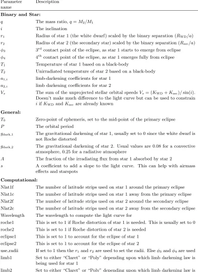
2.1 lcurveparameters . . . 36
3.1 Log of spectroscopic observations of NN Ser . . . 40
3.2 Photometric observations of NN Ser . . . 42
3.3 Comparison star information . . . 43
3.4 Identified emission lines in the UVES spectra . . . 54
3.5 Best fit parameters from MCMC minimisation . . . 56
3.6 Distance measurements for NN Ser . . . 58
3.7 Measured and corrected values ofKsec . . . 61
3.8 System parameters . . . 66
4.1 Observations of SDSS J0857+0342 . . . 69
4.2 Parameters from fitting the light curves of SDSS J0857+0342 . . . . 73
4.3 Hydrogen Balmer line offsets and velocities . . . 76
4.4 Parameters for SDSS J0857+0342 . . . 77
5.1 Journal of observations for GK Vir and SDSS J1212-0123 . . . 84
5.2 White dwarf absorption features in SDSS J1212-0123. . . 88
5.3 Secondary star atomic absorption features in SDSS J1212-0123 . . . 90
5.4 Fitted parameters for SDSS J1212-0123 . . . 94
5.5 Fitted parameters for GK Vir . . . 102
5.6 System parameters for SDSS J1212-0123 and GK Vir . . . 103
6.1 Mid-eclipse times for CSS 41177 . . . 111
6.2 Parameters for CSS 41177 . . . 115
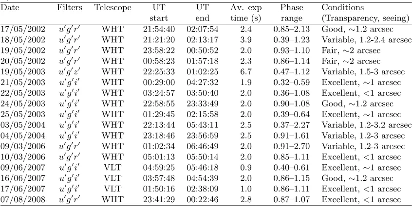
7.1 ULTRACAM observations of eclipsing PCEBs . . . 118
7.2 Non-ULTRACAM observations of eclipsing PCEBs . . . 119
7.3 Previously determined physical parameters . . . 123
A.1 Secondary star emission lines in SDSS J1212-0123 . . . 152
B.1 Secondary star emission lines in GK Vir . . . 155
C.1 ULTRACAM eclipse times for DE CVn . . . 159
C.2 Previous eclipse times for DE CVn . . . 160
C.3 ULTRACAM eclipse times for GK Vir . . . 161
C.4 Previous eclipse times for GK Vir . . . 162
C.5 ULTRACAM eclipse times for NN Ser . . . 163
C.6 Other eclipse times for NN Ser . . . 164
C.7 ULTRACAM eclipse times for QS Vir . . . 165
C.8 Other eclipse times for QS Vir . . . 166
C.9 ULTRACAM eclipse times for RR Cae . . . 167
C.10 Previous eclipse times for RR Cae . . . 168
C.11 ULTRACAM eclipse times for RX J2130.6+4710 . . . 169
C.12 Previous eclipse times for RX J2130.6+4710 . . . 170
C.13 ULTRACAM eclipse time for SDSS J0110+1326 . . . 171
C.14 Previous eclipse times for SDSS J0110+1326 . . . 172
C.15 ULTRACAM eclipse time for SDSS J0303+0054 . . . 173
C.16 Previous eclipse times for SDSS J0303+0054 . . . 174
C.17 ULTRACAM eclipse time for SDSS J1212-0123 . . . 175
C.18 Previous eclipse times for SDSS J1212-0123 . . . 176
List of Figures
1.1 Equipotential surfaces of the Roche geometry in a binary system . . 4
1.2 A third body’s effect on eclipse times . . . 11
2.1 Reading out a CCD . . . 13
2.2 Infrared detector readout modes . . . 14
2.3 ULTRACAM filter profiles . . . 15
2.4 CCD calibration frames . . . 17
2.5 A CCD image with apertures . . . 18
2.6 2D image of a stellar spectrum . . . 20
2.7 Telluric absorption . . . 22
2.8 A raw ´echelle spectrum . . . 23
2.9 Flat-fielding an ´echelle spectrum . . . 24
2.10 Line profile fit to the Ki7699 ˚A line . . . 25
2.11 Optical depth effects on emission lines . . . 28
2.12 Effects of optical depth on the light curve of a line . . . 29
2.13 The primary eclipse geometry in a PCEB . . . 32
2.14 Decreasing the radius-inclination correlation . . . 37
3.1 Average spectrum of NN Ser . . . 41
3.2 Sine curve fit for the Heii4686 ˚A absorption line . . . 44
3.3 Sine curve fit to the Balmer absorption features . . . 45
3.4 Normalised white dwarf spectrum of NN Ser . . . 46
3.5 Trailed spectra of various lines . . . 47
3.6 Sine curve fits for the Balmer emission features . . . 48
3.7 Linewidths of the emission lines . . . 49
3.8 Spectrum of the heated part of the secondary star . . . 50
3.9 Hydrogen emission line profiles . . . 51
3.12 Light curves of various emission lines . . . 60
3.13 Ksec correction applied to the emission lines . . . 62
3.14 Mass-radius plot for the white dwarf in NN Ser . . . 63
3.15 Mass-radius plot for the low mass star in NN Ser . . . 64
4.1 Spectral model fit to the white dwarf component of SDSS J0857+0342 71 4.2 Light curves of SDSS J0857+0342 . . . 72
4.3 Model fits to the lightcurves of SDSS J0857+0342 . . . 74
4.4 Averaged X-shooter spectrum . . . 74
4.5 Trailed spectrum of several lines . . . 75
4.6 Mass-radius plot for the white dwarf in SDSS J0857+0342 . . . 78
4.7 Mass-radius plot for the low mass star in SDSS J0857+0342 . . . 79
5.1 Averaged X-shooter spectrum of SDSS J1212-0123 . . . 85
5.2 Calcium and Magnesium absorption in SDSS J1212-0123 . . . 87
5.3 Trailed spectra of several lines in SDSS J1212-0123 . . . 88
5.4 Radial velocity fits to both components of SDSS J1212-0123 . . . 91
5.5 Equivalent width variations of the Ki7699˚A line in SDSS J1212-0123 91 5.6 Light curve fits for SDSS J1212-0123 . . . 94
5.7 Averaged X-shooter spectrum of GK Vir . . . 95
5.8 Trailed spectra of several lines in GK Vir . . . 97
5.9 Radial velocity fits to both components of GK Vir . . . 98
5.10 TheKsec for SDSS J1212-0123 and GK Vir . . . 100
5.11 Light curve fits for GK Vir . . . 101
5.12 Mass-radius plot for white dwarfs . . . 104
5.13 Mass-radius plot for the white dwarf in SDSS J1212-0123 . . . 106
5.14 Mass-radius plot for low-mass stars . . . 107
6.1 LT+RISE light curve of CSS 41177 . . . 111
6.2 Fit to the SDSS spectrum of CSS 41177 . . . 112
6.3 Trailed spectrum of CSS 41177 . . . 113
6.4 Constraints on the parameters of CSS 41177 . . . 115
7.1 Primary eclipses of DE CVn, QS Vir and RX J2130.6+4710 . . . 121
7.2 Primary eclipses of RR Cae, SDSS J0110+1326 and SDSS J0303+0054 122 7.3 Full orbit light curves of QS Vir . . . 124
7.4 Full orbit light curves of SDSS J0303+0054 . . . 126
7.5 Light curve and model fit to the eclipse of GK Vir . . . 129
7.7 O-C diagram for DE CVn . . . 131
7.8 O-C diagram for GK Vir . . . 132
7.9 O-C diagram for NN Ser . . . 134
7.10 O-C diagram for QS Vir . . . 136
7.11 O-C diagram for RR Cae . . . 139
7.12 Eclipse width as a function of O-C for NN Ser . . . 143
7.13 Variations in the secondary star scaled radii for GK Vir and NN Ser . 144 8.1 Mass-radius plot for white dwarfs . . . 148
Acknowledgments
I am extremely grateful to Prof. Tom Marsh for his support and guidance throughout my PhD. His ability to clearly explain any aspect transformed me from a graduate student into a researcher. His door was always open and I’ve lost count of the number of hours we’ve spent discussing various topics.
I thank Prof. Boris G¨ansicke, Dr. Chris Copperwheat and Stelios Pyrzas for a great number of enlightening discussions over the years. I would also like to thank the entire ULTRACAM team, particularly Prof. Vik Dhillon, for giving me the opportunity to use ULTRACAM and their trust in leaving it in my hands! There have been several occasions when I’ve had to call Vik in the middle of the night with some sort of problem and he was always able to solve it.
Declarations
I, Steven Parsons, hereby declare that this thesis has not been submitted in any previous application for a higher degree. This thesis represents my own work, except where references to other works are given. The following Chapters are based on refereed publications that I have submitted during my period of study:
Chapter 3 is based on: Parsons S. G., Marsh T. R., Copperwheat C. M., Dhillon V. S., Littlefair S. P., G¨ansicke B. T. and Hickman R., “Precise mass and radius values for the white dwarf and low mass M dwarf in the pre-cataclysmic binary NN Serpentis”, MNRAS, 402, 2591 (2010).
Chapter 4 is based on: Parsons S. G., Marsh T. R., G¨ansicke B. T., Dhillon V. S., Copperwheat C. M., Littlefair S. P., Pyrzas S., Drake A. J., Koester D., Schreiber M. R. and Rebassa-Mansergas A., “The shortest period detached white dwarf + main-sequence binary”, MNRAS, 419, 304 (2012).
Chapter 5 is based on: Parsons S. G., Marsh T. R., G¨ansicke B. T., Rebassa-Mansergas A., Dhillon V. S., Littlefair S. P., Copperwheat C. M., Hickman R. D. G., Burleigh M. R., Kerry P., Koester D, Nebot G´omez-Mor´an A., Pyrzas S., Savoury C. D. J., Schreiber M. R., Schmidtobreick L, Schwope A. D., Steele P. R. and Tappert C., “A precision study of two eclipsing white dwarf plus M dwarf binaries”, MNRAS, 420, 3281 (2012).
Chapter 6 is based on: Parsons S. G., Marsh T. R., G¨ansicke B. T., Drake A. J. and Koester D., “A Deeply Eclipsing Detached Double Helium White Dwarf Binary” ApJ, 735, L30 (2011).
Abstract
Recent years have seen an explosion in the number of eclipsing binaries containing white dwarfs. In the last few years the number of systems has increased from 7 to over 40, thanks mainly to large surveys such as the Sloan Digital Sky Survey and the Catalina Sky Survey. Many of these systems are survivors of the common envelope phase during which the two stars orbit within a single envelope which is rapidly thrown off through loss of energy and angular momentum. Detailed analysis of these systems can yield extremely precise physical parameters for both the white dwarf primary and its companion star. Stellar masses and radii are some of the most fundamental parameters in astronomy and can be used to test models of stellar structure and evolution. They can also be used to constrain the evolutionary history of the binary system offering us the chance to better understand the common envelope phase itself.
In this thesis I present high-precision studies of several eclipsing post common envelope binaries. I use a combination of high-speed photometry and high-resolution spectroscopy to measure the masses and radii of both stars in each system. I compare these results to evolutionary models and theoretical mass-radius relations and find that, on the whole, the measured masses and radii agree well with models. However, the main-sequence companion stars are generally oversized compared to evolutionary models, although this deviation is much less severe at very low masses (<
∼0.1 M⊙). I
also find that the measured masses and radii of carbon-oxygen core white dwarfs are in excellent agreement with theoretical models. Conversely, the first ever precision mass-radius measurement of a low-mass helium core white dwarf appears undersized compared to models.
Large scale surveys have also begun to identify double white dwarf eclipsing binaries. In this thesis I present a study of one of these systems and show the potential, as a double-lined spectroscopic binary, of measuring precise parameters for both stars in the future.
Chapter 1
Introduction
1.1
Prelude
The night sky has been used for thousands of years as a calender and navigational tool. In ancient Persia it was also used as an eye test. Mizar, one of the brightest stars in the Plough, has a faint partner named Alcor. The two stars appear virtually indistinguishable except to those with perfect eyesight. These two stars were in fact the first binary stars ever known (a recent study by Mamajek et al. 2010 has shown that these stars actually form part of a sextuplet system). We now know that most stars are part of binary or multiple systems (Iben, 1991). The majority of these stars are sufficiently separated from each other that they will never interact and will evolve in the same manner as an isolated star of the same mass.
plus main-sequence star systems. A small number of these systems are inclined in such a way that, as viewed from Earth, they exhibit eclipses. These detached eclips-ing binaries are a primary source of accurate physical properties of stars and stellar remnants. A combination of modeling their light curves and measuring the radial velocities of both components allows us to measure masses and radii to a precision of better than 1 per cent (e.g. Andersen 1991; Southworth et al. 2005; South-worth et al. 2007; Torres et al. 2010). These measurements are crucial for testing theoretical mass-radius relations, which are used in a wide range of astrophysical circumstances such as inferring accurate masses and radii of transiting exoplanets, calibrating stellar evolutionary models and understanding the late evolution of mass transferring binaries such as cataclysmic variables (Littlefair et al. 2008; Savoury et al. 2011). Additionally, the mass-radius relation for white dwarfs has played an important role in estimating the distance to globular clusters (Renzini et al., 1996) and the determination of the age of the galactic disk (Wood, 1992).
Although ubiquitous in the solar neighborhood, the fundamental properties of low-mass M dwarfs are not as well understood as those of more massive stars (Kraus et al., 2011). There is disagreement between models and observations, con-sistently resulting in radii up to 15 per cent larger and effective temperatures 400K or more below theoretical predictions (Ribas 2006; L´opez-Morales 2007). These in-consistencies are not only seen in M dwarf eclipsing binaries (Bayless & Orosz 2006; Kraus et al. 2011) but also in field stars (Berger et al. 2006; Morales et al. 2008) and the host stars of transiting extra-solar planets (Torres, 2007).
of it. However, in this case, it is only the gravitational redshift measurement that gives a truly independent mass-radius measurement, since the white dwarf radius determined from its parallax and the spectral modeling still rely to some extent on white dwarf models, and hence the mass-radius relation, therefore this approach is less direct when it comes to testing white dwarf mass-radius relations.
The small size of white dwarfs (roughly Earth-sized) means that the eclipse features are short and sharp. These allow us to measure extremely precise eclipse times. Accurate eclipse timings can reveal period changes; long term period de-creases are the result of genuine angular momentum loss from the binary, however, shorter timescale period modulation can be the result of many different mechanisms (see section 1.3). Orbital period variations can give us insights into binary evolution. This thesis presents high precision studies of eclipsing white dwarf binaries, the main aim being to measure precise model-independent parameters for both stars in the binary. The same data produce very accurate eclipse times which are analysed in search of period changes.
1.2
Binary star evolution
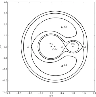
If two stars form a binary system, then their individual evolution may be affected by their companion. The combination of the gravitational potential of each star and the centrifugal potential create the potential of the system, known as the Roche geometry. Close to a star the equipotential surfaces are spherical and material is bound to the star. Further out the influence of the other star distorts the shape of the surfaces. The largest closed equipotential surface of each star is known as its Roche lobe. The lines of Roche equipotential depend only upon the mass ratio,
q = M1/M2, with the scale being set by a, the orbital separation (Warner, 1995),
an example of this is shown in Figure 1.1 for a binary with a mass ratio of 0.2. If the surface of both stars are well within their Roche lobes then they will remain spherical. However, as a star grows larger in radius it will begin to distort to match the equipotentials of its Roche lobe. The star becomes “pear” shaped and points towards its companion. If the star’s radius exceeds its Roche lobe then material will be transferred from the Roche lobe filling star to its companion via the inner Lagrangian point (L1) and mass transfer can being.
Figure 1.1: A cross section in the orbital plane of a binary with a mass ratio of 0.2, depicting the equipotential surfaces of the Roche geometry. The positions of the white dwarf (WD) and secondary star (MS) are shown as well as the centre of mass (CoM) and the five Lagrangian points (the points at which an object will be theoretically at rest relative to the two stars). The Inner Lagrangian point L1 lies
between the two masses. For the two outer Lagrangian points, L2 lies behind the
smaller mass, on the line determined by the two masses, and L3 lies behind the
larger mass. L4 and L5 are positioned at the vertical corners of the two equilateral
triangles with as shared base the line between the centres of the two stars, withL4
leading the motion of the orbit andL5 lagging behind. Thexandy axes are labeled
sphere containing the same volume as the Roche lobe is (Eggleton, 1983)
RL
a =
0.49q2/3
0.6q2/3 + ln 1 + q1/3. (1.1)
When the more massive member of a binary system departs from the main sequence and begins to expand, its surface may expand beyond its Roche lobe and material will be transferred to the less massive star. However, in this case material is moving from the more massive star to the less massive one and is therefore gaining angular momentum as it moves away from the centre of mass. To conserve angular momentum the binary separation must decrease, but this also leads to a reduction in the size of the Roche lobe by Equation 1.1.
If the donor has developed a deep convective envelope it can be approximated by a polytrope of index 1.5. In this case the mass-radius relation is R ∝ M−1/3,
hence its radius will expand in response to rapid (adiabatic) mass loss. This de-creases the timescale for mass transfer which will be well below the thermal timescale for the companion, even if it is a main-sequence star of comparable mass to the ini-tial mass of the donor (Iben & Livio, 1993). The companion is unable to readjust quickly enough to the additional mass and the accreted material simply piles up into a hot blanket on its surface until it too fills its Roche lobe, at which point a common envelope (CE) develops.
The envelope itself may not necessarily be rotating with the binary and therefore both stars will experience a drag force. This force causes the two stars to spiral inwards. The energetics that result in the ejection of the envelope of material are uncertain (Iben & Livio, 1993). However, a certain fraction of the orbital energy of the binary will be used to eject the common envelope. The parameter usually used to describe this isαCE (Webbink, 1984; de Kool et al., 1987; de Kool, 1992):
GMi(Mi−Mc)
Ri
=αCEλ
GMcM2
2af −
GMiM2
2ai !
, (1.2) whereλ is a parameter dependent upon the structure of the star, usually assumed to be constant, e.g. λ = 0.5 (de Kool et al., 1987). Mi and Ri are the mass and
radius of the star at the start of mass transfer, Mc is the core mass of the giant,
M2 is the companion star mass and ai and af are the separation of the two stars
before and after the common envelope phase. A value of αCE near unity implies
the current population of post common envelope binaries (PCEBs). The common envelope phase is thought to last<1000 years.
The core composition of the white dwarf that emerges from the CE phase depend upon the evolutionary status of the progenitor star. If the progenitor had not started helium burning then the white dwarf will have a He core with
MWD <∼ 0.5 M⊙. If helium burning was achieved then most of the helium would
have been converted to carbon and oxygen and the white dwarf will have a C/O core with a mass of 0.5 M⊙ <∼ MWD<∼ 1.1 M⊙. For the most massive white dwarfs
(1.1 M⊙ <∼MWD <∼1.38 M⊙) the progenitor would have been able to convert most
of the C/O to O/Ne and thus the white dwarf will have a O/Ne core.
1.2.1 Post common envelope binaries
Once the common envelope has been expelled the tightly bound binary is revealed containing the core of the giant, which will become a white dwarf, and its main-sequence companion. These binaries have periods of up to a few days.
Until recently only a handful of PCEBs (∼30) where known (see the cata-logue of Schreiber & G¨ansicke, 2003). This has now changed thanks mainly to the Sloan Digital Sky Survey (SDSS, York et al. 2000). A dedicated search for white dwarf plus main-sequence binaries in the SDSS spectroscopic survey yielded more than 1600 systems (Rebassa-Mansergas et al., 2007, 2010), of which roughly a third are PCEBs (Schreiber et al., 2008), based on radial velocity variations. The majority of these systems contain low-mass, late-type M dwarfs, while a large percentage of the white dwarfs are also of low mass (Rebassa-Mansergas et al., 2011). The sample of PCEBs has been further increased by long term photometric surveys such as the Catalina Sky Survey (CSS, Drake et al. 2009), which has identified over a dozen new eclipsing systems (Drake et al., 2010), and the Palomar Transient Factory (PTF, Law et al. 2009), which has also found several eclipsing systems with very dominant main-sequence stars (Law et al., 2011).
1.2.2 Double white dwarf binaries
Double white dwarf binaries (DWDs) share a similar evolutionary history to PCEBs. DWDs can be split into two groups which have different properties: the detached and semi-detached DWDs. In most cases DWDs are the result of a second common envelope phase, although an alternative channel for the formation of semi-detached DWDs involves a normal CV in which the mass transfer started from a donor close to the end of core hydrogen burning. In this case, mass transfer uncovers the helium-rich core of the donor and allows the system to avoid the classical period minimum of CVs at about 80 min (Solheim, 2010).
Detached DWDs are simple pairs of white dwarfs slowly spiraling towards each other under the influence of gravitational radiation. The semi-detached DWDs, known as AM CVn stars (see Solheim, 2010, for a recent review), are systems where mass is transferred from a Roche lobe filling hydrogen-deficient star to its more massive white dwarf companion. This mass transfer is stable and AM CVn binaries can reach very short periods, e.g. HM Cnc which has an orbital period of only 5.4 minutes (Israel et al., 2002; Roelofs et al., 2010).
Binary population synthesis studies predict that there are of order 100–300 million detached DWDs in the Galaxy (Han, 1998; Nelemans et al., 2001; Liu et al., 2010; Yu & Jeffery, 2010). They are likely to be the dominant source of background gravitational waves detectable by the proposed space-based gravitational wave in-terferometer, LISA (Hils et al., 1990). The loss of orbital angular momentum via gravitational radiation in these systems will eventually bring the two white dwarfs into contact with one another. Those that achieve this within a Hubble time are possible progenitors of AM CVn binaries, R CrB stars and Type Ia supernovae (Iben & Tutukov, 1984). The coalescence of two low-mass, helium core white dwarfs is also a possible formation channel for the creation of single sdB stars (Webbink, 1984); indeed it may be one of the more important sdB formation channels (Han et al., 2003).
(2010), Brown et al. (2011) and Vennes et al. (2011b) and an additional system presented in this thesis (Chapter 6).
1.3
Period change mechanisms
Angular momentum loss drives the evolution of close binary stars. For short period systems (<3 hours) gravitational radiation (Kraft et al. 1962; Faulkner 1971) dom-inates whilst for longer period systems (> 3 hours) a magnetised stellar wind can extract angular momentum, the so-called magnetic braking mechanism (Verbunt & Zwaan 1981; Rappaport et al. 1983). Accurate eclipse timings can reveal period changes; long term period decreases are the result of angular momentum loss, how-ever, shorter timescale period modulation can be the result of internal processes within the main sequence star, such as Applegate’s mechanism (Applegate 1992; see Section 1.3.3), or possible light travel time effects caused by the presence of a third body. Therefore, accurate eclipse timings of binaries can test theories of an-gular momentum loss as well as theories of stellar structure and potentially identify low mass companions. In this section I summarise the main mechanisms that can produce variations in the observed arrival time of eclipses.
1.3.1 Gravitational radiation
Angular momentum is lost from a binary system via gravitational radiation. The rate of angular momentum loss due to gravitational radiation was presented by Peters & Mathews (1963):
dJ dt =−
32 5
G7/2 c5 a
−7/2M2
1M22M1/2J, (1.3)
where ais the orbital separation, M1 and M2 are the primary and secondary star
masses andM is the total mass (M1+M2).
The relatively low masses of both stars in PCEBs mean that only a very small amount of angular momentum is lost via this mechanism. However, it does affect all binary systems and in some cases (e.g. the detached double white dwarf binaries) is the only mechanism that removes angular momentum from the system.
1.3.2 Magnetic braking
drag-down its rotation. In close binaries the rotational and orbital periods have become synchronised meaning that the angular momentum is taken from the binary orbit causing the period to decrease. In the disrupted magnetic braking model this process ceases in very low mass stars (M<
∼0.3M⊙) as it is hypothesised that they become
fully convective in this mass regime and hence the magnetic field is no longer rooted to the stellar core. This model was proposed to explain the cataclysmic variable period gap (a dearth of systems with periods between 2 and 3 hours). At periods of around 3 hours the secondary star becomes fully convective and hence magnetic braking ceases, this reduces the mass transfer rate and eventually causes the donor to shrink back to within its Roche lobe, stopping mass transfer. During this time the period loss is driven solely by gravitational radiation until the secondary star touches its Roche lobe again at a period of around 2 hours. However, it is still unclear how the angular momentum loss changes over the fully convective boundary (Andronov et al., 2003).
Verbunt & Zwaan (1981) calculated the angular momentum loss rate due to magnetic braking to be
dJ
dt =−3.8×10
−23
M⊙R⊙4M2Rγ2ω3J 0> γ >4 (1.4)
where ω is the angular frequency of rotation of the secondary star. γ is a di-mensionless parameter which can have a value between 0 and 4, in the context of cataclysmic variable evolution γ = 2 is frequently used (Schreiber & G¨ansicke, 2003). For PCEBs the angular momentum lost via magnetic braking is many orders of magnitude higher than via gravitational braking. However, for many systems the secondary star has a mass less than 0.3M⊙ (a fully convective atmosphere) and
hence magnetic braking should not be occurring.
1.3.3 Applegate’s mechanism
In Applegate’s mechanism (Applegate, 1992), as the main sequence star goes through an activity cycle, the outer parts of the star are subject to a magnetic torque chang-ing the distribution of angular momentum and thus its oblateness. The orbit of the stars are gravitationally coupled to variations in their shape hence the period is al-tered on the same timescale as the activity cycles. This has the effect of modulating the period with fairly large amplitudes (∆P/P ∼10−5) over timescales of decades
or longer.
mechanism and comparing it to the total amount of energy available to the main-sequence star. Applegate’s equation for the energy required to generate a period change is
∆E= Ωdr∆J+
∆J2
2Ieff
, (1.5)
where Ωdr is the initial differential rotation which is set to zero since we are after
the minimum energy required. The star is separated into a shell and a core,Ieff =
ISI∗/(IS+I∗) is the effective moment of inertia where S stands for the shell and∗
represents the core. Following the prescription of Applegate (1992) the shell mass is set toMS = 0.1M⊙meaning thatIeff = 0.5IS= (1/3)MSR∗2. The change in angular
momentum, ∆J, is calculated via ∆J = −GM
2
R
a
R
2 ∆P
6π , (1.6)
wherea is the orbital separation. The energy required for Applegate’s mechanism can then be compared with the total energy available to the main sequence star over the time-span of the period change (∆τ),
E= 4πR2σT4∆τ, (1.7) whereT is the temperature of the star andσis the Stefan-Boltzmann constant. If the total energy available is lower than the minimum required to drive the period change via Applegate’s mechanism, then an alternative explanation is required to explain the period change. However, even if the energy is available, it does not necessary mean that it is caused by Applegate’s mechanism, only that it is a possible cause.
1.3.4 Third bodies
The presence of a third body results in the central binary being displaced over the orbital period of the third body. This delays or advances eclipse times through variations in light travel time (see Figure 1.2). Since the third body can have a large range of orbital periods these effects can happen over a range of timescales.
1.4
Thesis overview
Figure 1.2: An invisible third body (black circle) in orbit around a close binary (blue+red circles) will cause a cyclic period change as observed from Earth. As the central binary moves around the centre of mass of the whole system (green point) it moves slightly further away from, or closer to, Earth. Therefore, the light has more or less distance to travel and as a consequence eclipses are observed to appear later or earlier than predicted.
related to close binary evolution and that eclipsing binaries are a powerful tool to use to help try and solve these problems. I have also shown that there are a variety of mechanisms that can affect the orbital period of a compact binary, both genuine angular momentum loss as well as other quasi-sinusoidal effects, and that the eclipses of compact binaries can be used to detect possible planetary mass companions.
Chapter 2
Methods and Techniques
2.1
Introduction
In this chapter I will outline all the techniques I used to analyse eclipsing white dwarf binaries. I will begin with discussing the basics of collecting and reducing astronomical data. I will then present several important tools for analysing eclipsing binaries with the aim of measuring fundamental parameters.
2.2
Observations and Reductions
2.2.1 Charge Coupled Devices
Charge Coupled Devices (CCDs) are the workhorses of modern astronomy. The low noise level, high quantum efficiency and wide bandpass of CCDs have made them almost ubiquitous. A CCD is a collection of metal-oxide semiconductor (MOS) capacitors in a two dimensional array, known as pixels. When a photon hits a pixel it produces an electron via the photoelectric effect. A voltage applied to the electrodes produces a potential barrier which traps the electron until the CCD is readout.
The CCD readout proceeds in the following way: first, the collected electrons are shifted across the array one column at a time, while the last column is shifted on to the serial register. The electrons are then moved down the serial register to the sense node, where the charge is measured and converted to a digital number, called an analog-to-digital unit (ADU). This process is repeated until the entire CCD is read out. The operation of a CCD can be summarised in thebucket brigade analogy, illustrated in Figure 2.1.
Figure 2.1: The “bucket brigade” analogy for the operation of a CCD. Each bucket (pixel) fills with rainwater (photo-electrons) during an exposure. Once the exposure is finished, each row of buckets is moved down one row at a time onto the serial register. Once on the serial register each bucket is moved to the sense node to measure the amount of rainwater. Figure courtesy of Richard Hickman.
This, combined with the additional noise introduced by spurious electrons in the on-board CCD electronics, is referred to as readout noise.
The charge transfer procedure can be very fast. However, the analog to digital conversion process is much slower and limits the readout speed of a CCD. The time taken for the CCD to readout is known as the dead time and can be quite significant, of the order of 2−100s (depending upon the number of pixels). There are several ways to reduce the dead time; binning can be used to group together several pixels and read them out together. For example, using a 2×2 binning mode will group 4 adjacent pixels together, reducing the overall readout time by a factor of∼4. Furthermore, windowing can be used to readout only a specific part of the CCD, the smaller the windows, the shorter the dead time.
Frame transfer CCDs use a different approach. In this case the CCD has an extra unexposed area which can be read whilst the next exposure is being made. In this way the dead time can be greatly reduced. For example, the frame transfer CCDs used by the high-speed camera ULTRACAM (Dhillon et al., 2007) are capable of transferring the frame in milliseconds whilst the time to read the entire CCD is
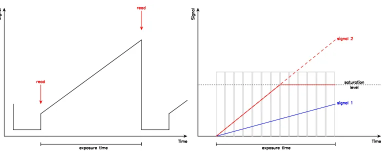
Figure 2.2: Infrared detector readout modes. Left: an example of Double Correlated Read mode. The charge is read out at the start and end of the exposure, eliminating any offsets, such as thermal noise. Right: an example of Non-Destructive Read. The charge is sampled several times during the exposure and the count level is determined by fitting the slope of the Signal vs. Time. For pixels with high flux (red) only the readout values below the saturation level are taken into account when calculating the slope. The pixel value is then extrapolated to the full exposure time.
2.2.2 Infrared Detectors
Unlike optical CCDs, the charges from individual pixels in infrared detector arrays are not shifted from pixel to pixel during the readout process. Attempts to make charge transfer devices from infrared detector materials have been generally unsuc-cessful (Joyce, 1992). Instead, each pixel is independently read and each column individually reset. This allows several different readout methods. The two most common infrared detector readout modes are:
Double Correlated Read: In Double Correlated Read (DCR) the voltage is sampled twice, once at the beginning of the exposure and a second time at the end of the exposure. This approach eliminates thermal noise and other offsets, but increases the read noise by√2 because the noise from both readouts go into a single image. DCR incurs fewer overheads and thus is suitable where the dominant source of uncertainty is the Poisson noise of the sky emission, e.g. infrared imaging. An example of DCR is shown in the left hand panel of Figure 2.2
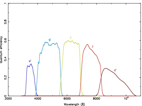
Figure 2.3: ULTRACAM filter profiles (including the quantum efficiency of the detectors). Only light within a specific wavelength range is permitted through to the detector. This allows flux measurements with different instruments to be directly compared.
threshold (close to the detector saturation) and extrapolating to the exposure time. The sampling need not be linear, sampling concentrated towards the beginning and end of the integration minimises the noise and is known as Fowler sampling (Fowler & Gatley, 1990). An example of NDR is shown in the right hand panel of Figure 2.2, with regularly spaced sampling.
The SOFI photometry presented in Chapters 4 and 5 uses DCR mode, whilst the near infrared data from X-Shooter also presented in Chapters 4 and 5 were collected using NDR mode with threshold limited integrations.
2.2.3 Photometry
is accurate. The following sections outline these steps.
Bias subtraction
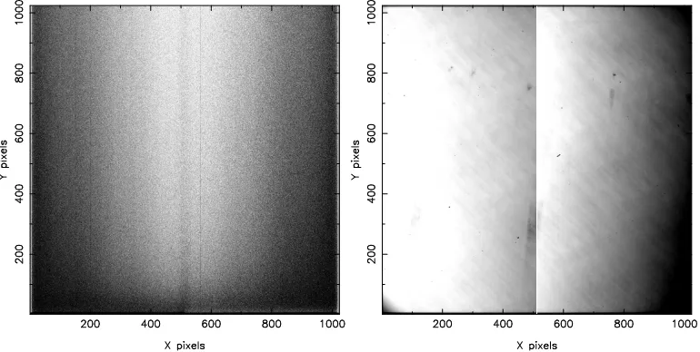
Since the analog to digital conversion process introduces a small amount of sta-tistical fluctuation in the pixel values, the zero value of the CCD is offset. This avoids potential negative pixel values (which would require a “sign bit” to be used). However, this bias level needs to be subtracted so that errors can be properly deter-mined. This can be estimated by using a bias frame which is a zero exposure-time frame, an example of which is shown in the left hand panel of Figure 2.4. Several bias frames can be combined to reduce the statistical noise and the resultant frame subtracted from the science images.
Bias frames are not possible using infrared detectors since zero second expo-sures are not possible. Therefore, any bias level is subtracted using dark frames.
Dark-current subtraction
Electrons in the detector can occasionally gain enough thermal energy to jump into the conduction band without the influence of a photon. This extra signal is known as the dark current and can be a substantial source of noise, especially for long exposures. The dark current can be reduced by cooling the detector. An estimate of the dark current can be made using dark frames, which are long exposures with the shutter closed. For CCDs the dark current is proportional to the exposure time, therefore the dark frame can be scaled to match the exposure time of the science image. Infrared detector materials have a dark current that is not linear with time and hence dark frames must be taken with the same exposure time as the science frames. Usually several dark frames are combined to reduce the statistical noise and the resultant frame is subtracted from the science frames. For CCDs the bias level is removed before subtraction whilst the dark frame of an infrared detector acts as both a dark and bias frame.
Flat-fielding
Figure 2.4: left: a bias frame from CCD2 of ULTRACAM. The CCD is split into two channels with different bias levels, here the left hand channel has been multiplied up to match the mean level of the right hand one. The difference between the highest and lowest value is only 3%. Right: a flat field frame from CCD2 (g′
band) of ULTRACAM.
one. All science images are then divided by this frame. Alternately, special flat field screens are provided in many observatories (known as dome flats). An example of a flat field frame is shown in the right hand panel of Figure 2.4.
Aperture photometry
Figure 2.5: An NTT+ULTRACAM g′
band image of the sky with several stars visible. The CCD was windowed and only half is shown. Three stars have apertures placed over them. For each star, the smallest circle is the object aperture whilst the two larger circles denote the sky annulus.
The usual way of choosing the size (radius) of the apertures is profile fitting. This approach assumes that the profile of the star resembles some known function (e.g. Gaussian or Moffat functions, the latter based on stellar images (Moffat, 1969)) and thus we can fit the profile to measure variables such as peak intensity and Full-Width at Half-Maximum (FWHM). This allows us to get a good idea of the current atmospheric conditions. The size of the apertures is then based on the FWHM multiplied by a suitable scaling factor. Initially a range of scale factors are used (e.g. ranging from 1.5 to 2.0, in steps of 0.1), then the scale factor that produces the highest signal-to-noise ratio is chosen for the final reduction.
Differential photometry
Flux calibration
In some cases it is desirable to turn count values into magnitudes or milli-Janskys (mJy). These values can be compared to external data sets and models. This conversion is achieved using a standard star. Standard stars are relatively bright, non-variable stars with well measured magnitudes in several different bands. The list presented by Smith et al. (2002) is generally used to flux calibrate observations made with the SDSSugriz filters.
The magnitude of the standard star is
mµ=−2.5 log10(Cµ) +xµ−κµX, (2.1)
where µ represents the filter of interest, Cµ is the counts per second, xµ is the
instrumental zero point, κµ is the extinction coefficient in theµband and X is the
airmass.
Since the magnitude of a standard star is known, the only unknowns are the instrumental zero point and the extinction coefficient. A theoretical extinction coefficient can be used but it can also be measured. Using a long observing run (covering a large range in airmass), a linear fit to counts vs. airmass yields the extinction coefficient. Once this is measured the zero point can be obtained and applied to the comparison star and hence the object itself.
To ensure an accurate flux calibration, large apertures must be used to ensure that all the flux is collected. The usual method used to flux calibrate a target’s light curves is to use the longest run on the target to determine the comparison star’s magnitude. Once determined, the comparison star’s magnitude is then fixed and used to flux calibrate all other observations of that target.
2.2.4 Spectroscopy
Spectroscopy involves measuring the flux of an object over a range of wavelengths. This technique can yield information impossible to measure with photometry. Spec-troscopic observations are performed using a spectrograph. In a spectrograph the light is first passed through a slit, located at the focus of the telescope. The diver-gent beam is collimated by a collimator mirror (or lens) and sent to a dispersing element, usually a diffraction grating. The diffracted light is then sent to a camera which focuses it onto a detector (e.g a CCD).
Figure 2.6: Raw image of a stellar spectrum taken using GMOS on the Gemini North Telescope. The star is the bright line across the centre, sky emission lines run perpendicular to it. The dark region x <35 is an overscan region and can be used to estimate the bias level. The sky level will be measured between the green lines whilst the star’s flux will be measured between the red lines.
sections outline the calibration steps for reducing spectroscopic data.
Bias and dark-current subtraction
Bias subtraction and dark current removal are performed in the same way as pho-tometric reduction. Most spectrographs have an extended region on the chip which is not exposed to light. This overscan region can be used to measure the bias level for each frame individually (Figure 2.6).
Flat-fielding
The concept of flat-fielding remains the same for spectroscopic data, although there are slight differences. Flat field spectra are usually obtained using a Tungsten lamp located inside the spectrograph. However, the Tungsten spectrum in not flat since it is modulated by its intrinsic, blackbody-like spectrum. Therefore, the flat field frame is collapsed along the spatial direction and the 1D spectrum is fitted with a polynomial. The 2D frame is then divided by the polynomial and applied to the science frames.
Spectrum extraction
column a polynomial is fitted to the sky and interpolated in the region containing the target spectrum. A profile is fitted to the target region, this profile is used to assign weights to each pixel. Finally, the background is subtracted and the object extracted using the determined weights in the method outlined by Marsh (1989).
Wavelength calibration
In order to properly analyse the extracted spectrum we need to convert the x-axis from pixels to wavelength. This is achieved by extracting an arc spectrum. These are exposures of emission line lamps with numerous spectral lines with precisely known wavelengths. Examples are CuNe, CuAr or ThAr lamps. The position of each identified line is fitted and compared to the reference wavelength. A polynomial (usually of order 5-7) is fitted to determine the transformation between pixels and wavelength. This transformation is then applied to the science spectra.
Often the arcs will drift during the night, and can be affected by the position of the telescope. Common practice is to observe an arc spectrum both before and after the science exposure and interpolate in time between them for the science spectrum.
Flux calibration
Similar to photometry, the conversion from counts to flux units requires the obser-vation of a standard star. For spectroscopy these spectrophotometric standards are constant stellar sources with well known spectra, observed using a wide slit. The observed spectrum is compared to the template spectrum and the difference is fit-ted with a spline. The fit is then applied to the science spectra. This approach can remove the instrumental response fairly well. However, since most science spectra are taken with a narrow slit (to achieve the best resolution), some of the light from the target is lost on the slit. These slit losses, and variations in conditions, make absolute flux calibration of variable sources difficult.
Figure 2.7: A spectrum of the B7 starσAri, showing both real features (the hydro-gen Paschen series) and telluric absorption features.
extinction across the wavelength range, as well as variations in seeing.
Telluric correction
The Earth’s atmosphere is not completely transparent, even in the visual wavelength range. Figure 2.7 shows forests of lines appearing at∼6900˚A,∼7600˚A and∼9500˚A as well as other places throughout the spectrum. These are caused by oxygen and water vapour in the atmosphere and may need to be corrected for in some cases, this is particularly important for the sodium doublet at∼8200˚A.
Telluric standards are used to correct for these features. These are observa-tions of stars with relatively featureless spectra. The telluric spectrum is continuum normalised, using a spline fit or model spectrum, leaving just the telluric features. One problem is that many of the absorption features are saturated and hence their strength will not be linearly proportional to airmass. This can be somewhat cor-rected for by using a power law scaling, or trying to minimise the scatter in a well defined telluric region (e.g. the deep feature at ∼ 7600˚A). This only really works for low to medium resolution data. Applying a telluric correction can restore the original shape of the spectrum, but these regions are much noisier due to the lower number of original counts.
´
Echelle spectroscopy
´
Figure 2.8: A raw ´echelle spectrum taken using X-Shooter at the VLT. The object spectrum is the dark, highly curved lines in the centre of each order. There are 16 orders in total, with the shortest wavelengths at the bottom. Also visible are a num-ber of sky lines running perpendicular to the objects spectrum. This image covers the NIR region (1.0−2.5 microns) and the deepJ and H atmospheric absorption bands are visible in the 8th and 13th orders up.
orders. An example of a raw ´echelle spectrum taken using X-Shooter is shown in Figure 2.8. X-Shooter (D’Odorico et al., 2006) is a medium resolution spectrograph and works at diffraction orders ofn ∼20 (c.f. the high resolution ´echelle spectro-graph UVES (Dekker et al., 2000) which works at n ∼ 120). In Figure 2.8, the bottom order is in fact the highest order (n= 26) and contains the shortest wave-length information. The order above this (n= 25) contains longer wavelength data, but there is a region of wavelength overlap.
´
Echelle spectroscopy requires two additional steps beyond those used for normal spectroscopy. Firstly, each order must be identified and traced. For the highly curved orders seen in X-Shooter this requires resampling each order. The transformation from pixels to wavelength and slit height must be calculated for each order. Secondly, the orders must be combined. A weighted average is usually used for those wavelengths in the overlap regions.
Figure 2.9: Left: a non-flat fielded ´echelle spectrum of a white dwarf. Right: the same spectrum but divided by the flat field frame. This demonstrates the importance of using a flat field frame to correct for the blaze function.
often be seen in the final spectrum (this is a particularly large problem for UVES data). We can attempt to remove this ripple by fitting it with a sinusoid of the form
B(λ) = a0+a1sin(2πφ) +a2λsin(2πφ) (2.2)
+a3cos(2πφ) +a4λcos(2πφ).
The phase (φ) can be calculated by identifying the central wavelength of each echelle order. Then using the relation
λn(O−n) =c, (2.3)
wherec and O are constants and λn is the central wavelength of order n, gives us
the phase. Since the phase is now known, Equation 2.2 reduces to a simple linear fit.
2.3
General tools
In the following sections I will outline some of the main tools that I use throughout this thesis. These are all techniques used for analysing binary systems.
2.3.1 Measuring radial velocities
Figure 2.10: Line profile fit to the Ki7699 ˚A absorption line originating from the
secondary star in the eclipsing PCEB SDSS J1212-0123. The line was fitted with a combination of a second-order polynomial and a Gaussian (red line). The velocity scale is centred on the rest wavelength of this line (7698.964˚A) and a small shift (∼70km s−1) is seen in the observed line position.
we spectroscopically observe a binary system over its entire orbit, we will see any spectral lines move. This is because the stars themselves are moving around the centre of mass and thus their spectra will be shifted due to the Dopper effect. This shift will correspond to the radial velocity (the projected velocity in the line of sight) of the star. The velocity of a spectral line can be determined by measuring its central wavelength,λobs, and comparing it to the lines rest wavelength,λ0. The
velocity of the line is thenV = c(λobs − λ0)/λ0. For circular orbits, the measured
velocity of a line will exhibit a sinusoidal variation over the course of an orbit, given by,
V(t) =γ+Ksin
2π(t
−T0)
P
(2.4) where γ is the systemic velocity, K is the radial velocity, P is the period of the binary and T0 is the zero-point of the ephemeris (i.e. the centre of the primary
eclipse). The ephemerides of all of the systems presented in this thesis are well known from photometry. Therefore,T0 and P are kept fixed for all radial velocity
measurements. However, Equation 2.4 shows that spectral lines can be used to determine the ephemeris of a binary.
potassium absorption line in SDSS J1212-0123 (presented in detail in Chapter 5). In this case I have used a Gaussian profile combined with a second-order polynomial to fit the line. In most cases a Gaussian fit is sufficient. However, the hydrogen Balmer lines seen in white dwarfs are highly pressure broadened due to the high gravity environment in a white dwarf atmosphere. Pressure broadening has a Lorentzian profile, therefore the wings of the line are more affected than the cores, leading to very wide (several thousand km s−1
) wings in these lines. Fortunately, the lower energy lines in white dwarfs (e.g. Hα) usually display sharp cores (2−3˚A in width) as the result of non-LTE effects (Greenstein & Peterson, 1973) which are useful for tracing their motion.
As well as the cores of the Balmer lines, white dwarfs in PCEBs often ac-crete a small amount of the wind from the secondary star. This can create narrow calcium and magnesium absorption lines ideal for radial velocity measurements. The low mass secondary stars in PCEBs are usually M dwarfs and therefore the sodium doublet at ∼ 8200˚A is usually used to measure their radial velocity. One complication here is that these lines lie in an area of relatively high atmospheric absorption and a telluric correction must be applied. The spectra of M dwarfs also display molecular absorption bands (e.g. TiO). Although these also track the mo-tion of the star, they are highly asymmetric and the central wavelengths are often unknown. Hence profile fitting of these features will not yield particularly accurate radial velocities.
Alternatively, a template spectrum can be used to measure radial velocities by cross correlating it with the observed spectrum. However, given the large number of strong, clean lines present in PCEBs, fitting the line profiles gives results to a similar precision, but is a much faster method then cross correlation.
2.3.2 Ksec correction
As well as absorption lines, spectra of PCEBs can contain emission lines. These emission lines usually originate from the heated face of a highly irradiated secondary star (i.e. those systems containing hot white dwarfs).
analytically as (Wade & Horne, 1988)
Ksec=
Kemis
1−f(1 +q)Rsec
a
, (2.5)
where Ksec is the centre of mass radial velocity, Kemis is the radial velocity of the
emission line,qis the mass ratio,Rsec/ais the radius of the secondary star scaled by
the orbital separation andf is a constant between 0 and 1 which depends upon the location of the centre of light. Forf = 0 the emission is spread uniformly across the entire surface of the secondary star and therefore the centre of light is the same as the centre of mass. Forf = 1 all of the flux is assumed to come from the substellar point.
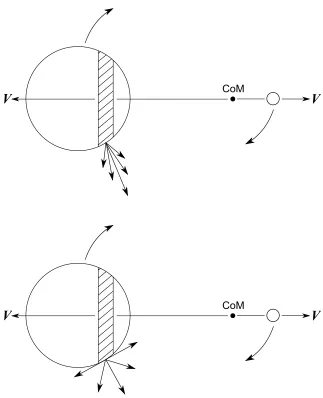
The measured radial velocity amplitude of an emission line will depend upon the optical depths of the line, which will affect the angular distribution of line flux from any given point on the star. This is illustrated in Figure 2.11. Differences in optical depth will also affect the light curve of the line for the same reasons. Fig-ure 2.12 shows the light curve of an optically thick and thin emission line. Therefore, we can use the light curve of a line to determine its optical depth and hence the
Ksec correction for that line.
We wanted to be able to model optically thin and optically thick emitting regions within one model so that there was a continuous transition from one to the other. To do so we assumed a simple model in which the line emitting region at any point on the secondary behaves as if it had a total vertical optical depth τ0, and a
source function given by an exponential function of vertical optical depth,τ,
S(τ)∝eβτ,
where β is a user-defined constant allowing the source function to increase or de-crease with optical depth. To prevent divergent integrals, we must have thatβ <1. For β > 0, the source function increases as one goes further into the star and we expect limb darkening, while β < 0 gives limb brightening. As τ0 → 0, we obtain
optically-thin behaviour, thus this two-parameter model gives the desired modeling freedom.
For an incident angle θ such that µ = cosθ, the emergent intensity is then given by
I(µ)∝
Z τ0
0 e
βτe−τ /µdτ
µ ,
V
CoM
V
V
CoM
[image:46.595.158.481.141.539.2]V
Figure 2.12: The effects of optical depth on the light curve of a line. In the optically thin case the emission is distributed uniformly meaning that the light curve is wider and flatter. In the optically thick case the light emitted at angles close to the stellar surface is reduced, meaning that the brightest region (the substellar point) contributes much less away from phase 0.5, compared to the optically thin case.
depth along the line of sight isτ /µ. Therefore
I(µ)∝ 1−e
(β−1/µ)τ 0
1−βµ .
In the limitτ0 → ∞ we have
I(µ)∝ 1
1−βµ,
which for small β gives I(µ) ∝ 1 +βµ, giving limb-darkening or brightening as expected. In the optically thin limit,τ0 →0,
I(µ)∝ τ0
µ.
Theµdivides out with theµfactor from Lambert’s law, and we find that each unit area contributes equally to all directions, as long as it remains visible. This enhances the star’s limb compared to the optically thick case. At quadrature for example, this will enhance emission from the sub-stellar point, leading to a low semi-amplitude.
2.3.3 Time system conversions
by Earth’s orbit around the Sun and the resulting run of the seasons, the month by the Moon’s movement around the Earth and the change of the Moon phases, the day by Earth’s rotation and the succession of brightness and darkness. Problems arise when high-precision times are required. Not only must one correct for the location on Earth, but one must also correct for the motion of Earth itself. These corrections can be up to several minutes and since we are able to measure eclipse times in PCEBs to sub-second accuracies it is vital that we make these corrections. This section outlines the main time systems used in modern astronomy and their relations to one another.
Universal Time (UT) was introduced in 1926 to replace the less stringent Greenwich Mean Time (GMT). However, this first version of UT, known as UT0, did not take into account the motion of the Earth’s poles. Correcting for this effect, one obtains UT1, which is equivalent across the entire surface of the Earth. One problem with UT1 is that the derived length of a second varies noticeably (due to irregularities in the Earths rotation). Therefore, in 1961 Coordinated Universal Time (UTC, a compromise between the English and French acronyms) was devised in which the SI second is the unit of time. UTC and UT1 are kept to within a second of one another by adding or subtracting leap seconds (although none have yet been subtracted). These are inserted into the last minute of June 30th or December 31st. The last leap second (as of 2012) was added on 31st of December 2008.
The SI second is defined as 9,192,631,770 cycles of a hyperfine transition in the ground state of133Cs, set to best match the previous definition of a second. Devices that attempt to measure the SI-second are known as atomic clocks. There are many atomic clocks located across the world and the mean time of all of these is known as Atomic Time (TAI). Due to the addition of leap seconds TAI currently (2012) runs 34 seconds ahead of UTC i.e.
UTC = TAI−N, (2.6) whereN is the number of leap seconds.
Terrestrial Time (TT) was introduced in 1991 as a uniform time system (replacing terrestrial dynamical time, which itself had replaced ephemeris time) and was needed to predict the positions of the Sun, Moon and planets. This is because the application of the laws of motion required a smoothly flowing time system. To millisecond accuracy, TT runs parallel to TAI but, for historical reasons, is 32.184 seconds ahead