Predicting demand of replacement cars for breakdown cases using machine learning techniques

PREDICTING DEMAND OF REPLACEMENT

CARS FOR BREAKDOWN CASES USING

MACHINE LEARNING TECHNIQUES

Siti Yaumi Salamah

Master Business Information Technology

Faculty of Electrical Engineering, Mathematics & Computer Science

August 2019

GRADUATION COMMITTEE

Maurice van Keulen

Faculty EEMCS, University of Twente

Adina Aldea

Faculty BMS, University of Twente

Chantal Epskamp

ANWB

2

A

BSTRACT

3

C

ONTENTS

Abstract ... 2

Contents ... 3

List of Figures ... 4

1 Introduction ... 5

1.1 Motivation ... 5

1.2 Case Description ... 6

1.3 Research Questions ... 7

1.4 Research Methodology ... 8

1.5 Thesis Structure ... 10

2 Background & Related Works ... 11

3 Methods ... 12

4 Dataset Creation ... 13

5 Demand Prediction Model ... 14

6 Putting the Model into Practice ... 15

7 Discussion, Limitations, and Future Work ... 16

8 Conclusions & Contributions ... 17

8.1 Conclusions ... 17

8.2 Contributions ... 19

4

L

IST OF

F

IGURES

5

1

I

NTRODUCTION

1.1

M

A vehicle breakdown is a mechanical defect of a motor vehicle in such a way that the failure prevents the vehicle from running or where continuing being operated is not safe. This incident can arise in various occasions, such as during travelling for holiday or work, even when the vehicle is not in use. There are numerous reasons for a vehicle breakdown, from a dead battery, fuel, ignition, to other mechanical problems. In a case of breakdown, driver and passengers’ convenience and safety can be at risk. In this situation, roadside assistance has come in handy, providing breakdown service that oftentimes cannot be done by the driver or passengers of the vehicle themselves and is in need of an expert skill to deal with the failure.

Every year, there are more than 1 million breakdown incidents recorded in the Netherlands (ANWB, 2019). However, not all vehicle faults can be repaired by the road patrols on the spot. In such cases, roadside assistance providers provided transport assistance to tow away the vehicles to a garage for reparation and bring the passengers to a destination. In addition, replacement vehicles (i.e. rental cars) can be provided for the customers while the cars are being repaired.

The whole processes form a complex workflow involving several parties, starting from receiving the incident report from a driver to possibly picking up and returning a rental car. It becomes a challenge for roadside assistance providers to ensure customer satisfaction along the line, starting from the emergency call service, roadside assistance, transport, and rental car services. Roadside assistance providers need to deal with not only resources and capacity planning for the roadside assistance process, but also for the replacement vehicles. Providers of the replacement vehicles need to optimize the number of available rental cars so that customers’ needs are fulfilled as fast as possible even during the peak season, while not leaving a lot of cars idle.

On top of that, among the processes along the line, car rental logistics is a complex problem which is difficult to deal with. A lot of effort has gone into studying the optimization of rental cars capacity and fleet management (Fink & Reiners, 2006; Yang et al., 2008; Gupta & Pathak, 2014; Oliviera et al., 2017a; Roy et al., 2014).

6 Despite some similarities of characteristics with the conventional car rental companies, rental car companies that provide replacement cars as their core business process also have a distinct characteristic and cannot be treated completely the same as the conventional rental car companies. The demand for rental vehicles in the context of vehicles breakdown is not only affected by customer behavior such as travelling pattern and busy commuting hours, but also by the factors that might affect the severity of car breakdown or the capability to quickly repair a car, which in result might end up with the need of replacement vehicles, i.e. the rental vehicles. To the best of our knowledge, little to no literature have covered the prediction of demand for such industry.

Lots of existing literature with car rental logistics as the use case consider the demand forecasting problems as a traditional time series forecasting problem (Pachon et al., 2006; Hong et al., 2007). They consider historical data and attributes of the time series, such as trend and seasonality for the forecast. In another literature, an intervention from analyst is expected to adjust the forecast in the existence of special events (Geraghty & Johnson, 1997).

Besides the traditional time series forecasting technique, time series forecasting can also be analyzed as a machine learning problem, specifically the supervised learning problem. Time series problem can be restructured into a supervised learning problem, thus allowing us to extract more valuable features from a timestamp and include external data as the factors that will affect demand prediction result. Therefore, factors like special events, holidays, and weather can be incorporated into the demand forecasting model and the linear and non-linear relationship of these features can be examined by using machine learning techniques. Research on machine learning-based demand forecasting dates back to the early 2000s and machine learning techniques have been shown to be valuable in getting a more accurate demand forecast.

However, despite the accuracy a machine learning technique can produce, there is a limitation in a predictability of demand given the nature of it. One would expect to find uncertainty in a demand forecast as there are typically discrepancies between forecasts and actual values (Ericsson, 2001) due to the uncertainty in input values (McKay, 1995), which can include a lot of factors, from human behavior to environment related factors. Therefore, there is a need in providing a measure of uncertainty for the decision makers to base their predictions on. One way to communicate uncertainty is by using forecast intervals as they generalize point forecasts to represent and incorporate uncertainty (Hansen, 2006). However, in machine learning forecasting, the capability to specify uncertainty or intervals are rarely included in the research agenda in the field (Makridakis et al., 2018).

Therefore, in this study we want to address the applicability of machine learning forecasting in the specific domain of replacement cars, which has not been a focus of any previous works. We first investigate the predictability of the demand of rental cars as a means of replacement vehicle in the case of unrepairable breakdown by utilizing available machine learning techniques to build a prediction model. In addition, we aim to produce a measure of forecast uncertainty through intervals as an essential part of demand forecast in practice. We compare several approaches to create the intervals and reflect on the strengths and weaknesses of each interval with regards to the quality and the applicability in the practice.

1.2

C

D

7 market consists of customers with direct membership subscription to ANWB, while B2B market consists of customers that are entitled to ANWB services through their contracts to another company that has a partnership with ANWB. Depending on the contracts, customers are provided with different kind of services, for example different types of replacement cars for when a breakdown cannot be solved on the spot or different duration for which the cars are rented to the customers.

To provide replacement vehicles for its customers, ANWB partner up with Logicx, its daughter company handling towing and replacement vehicles. Logicx´s fleet for the Netherlands is distributed in 85 locations owned by Logicx and its partners. In the event of unsolved breakdown problems, ANWB send a request for replacement cars to Logicx which then assign an available car from the pick-up location closest to the breakdown location or the most convenient location for the customer.

Each pick-up location has different maximum capacity of cars that it can keep in the location, from 2 up two 120 cars per location. To keep up with the demand, Logicx monitor the demand of replacement cars and the number of cars that are away and returned regularly. In case of shortage of cars in a certain location, Logicx can either transport cars from the other pick-up locations or outsource cars to another car rental company, Hertz, that will take about half a day lead time.

Moreover, the rented cars can be returned in any Logicx and partner locations and it can be different from the pick-up location. To deal with this, Logicx take care of the repositioning of the cars from one location to another location. Logicx plan and monitor this activity weekly and daily. The goal is to have an optimum number of cars in each location to avoid extra outsourcing or daily transportation cost, while keeping a low number of idle cars.

In addition to operational efficiency, ANWB want to ensure high level customer satisfaction with regards to the replacement vehicle service. One way to deal with this is by supporting Logicx with a demand forecast that can help them plan the distribution of cars such that customers can always pick up rental cars from the closest location to the breakdown incidents without long waiting time.

1.3

R

Q

Given the above-mentioned problem, the objective of this study is to predict the demand of replacement cars using machine learning techniques to enhance car rental logistics planning. The following research question was formulated in order to achieve this objective:

To what extent can we predict the demand of replacement cars in the Netherlands?

To answer the main research question, the following sub questions were defined:

SQ1. What features can be used to predict the demand of replacement cars?

8 SQ2. Which machine learning model is best suited to predict the demand of replacement cars?

We first conducted a literature review to get an overview of techniques that have been used for the problem. Then, to answer SQ2, a set of available techniques with the most suitable characteristics for the problem were selected. After that, these techniques were applied to build the predictive models and the models were evaluated based on their error performances. We then chose the best performing model and reflect on its strengths and weaknesses in regard to the case.

SQ3. What aggregation level works best for the demand prediction?

To answer SQ3, we built the demand prediction model in several levels of granularity, both for the product type and the spatial aggregation level. We then compared the performance of the prediction model from different aggregation levels.

SQ4. How can we estimate uncertainty of the prediction result?

To answer SQ4, we conducted literature review on the techniques that can be used to provide intervals for machine learning-based predictive model. Then, we selected a suitable measurement, compared several approaches and chose one that is most suitable to the case to provide upper and lower bounds in addition to the prediction results.

After answering each sub-question, we concluded the answer to the main research question by presenting the best performance of the replacement car demand prediction in the Netherlands that can be achieved using the analyzed features and the machine learning models considered.

1.4

R

M

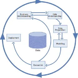
In this research, we used the widely adopted framework for data mining and analysis in industry, namely the CRISP-DM (Cross-Industry Standard Process for Data Mining). This standard process model supports best practices and is industry-, tool-, and application-neutral (Shearer, 2000). Figure 1 presents the six phases in the life cycle of a data mining project defined in the CRISP-DM framework.

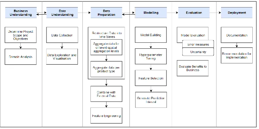
9 According to the CRISP-DM, the arrows between the phases show the most important and frequent dependencies between phases. The next process to perform depends on the outcome of the previous one. This concept supports the fact that many data science projects demand an iterative process, allowing one to go back and forth testing different schemes such as to include new features for the model. Therefore, referring to the six phases of the CRISP-DM, we set out an outline of the tasks to be carried out in this study as shown in Figure 2.

Figure 2 Research outline

The following is the description of the tasks in each phase of CRISP-DM. A more detailed explanation of the methods employed to conduct each step is provided in Chapter 3.

1. Business Understanding

The initial phase focuses on identifying the scope and objectives of the project. The research starts with a literature review of previous works and related topics to investigate the state of the art of the current research and understand the context of the problem. Then, we determine the project objectives according to the problem. We conduct initial assessment of tools and techniques and create the project plan. Domain analysis via interview with domain experts are also carried out to understand the business and gain the knowledge about the input factors that are important to the problem.

2. Data Understanding

This phase starts with initial data collection. After that, data exploration and descriptive analytics are conducted to find out the quality of the data, discover first insights, and investigate hypotheses from business understanding phase.

3. Data Preparation

10 4. Modeling

At this stage in the project, various modeling techniques are selected after conducting literature review and elimination by aspects to find several techniques suitable for the project. Then, we build and validate each model using the dataset created in the previous phase, including selecting the hyperparameters and the features for the model. We test the model and then produce prediction interval for the model.

5. Evaluation

The evaluation phase covers the evaluation of several models resulted in the modeling phase by comparing their performances. In this study, in addition to the error of the model, we evaluate the uncertainty of the model represented by the prediction intervals. Then, we relate it to the practice to determine if the business issue has been addressed sufficiently and if the project objectives have been achieved. We review the processes, determine a list of alternative next steps and draw the conclusions of the study.

6. Deployment

For the deployment stage, we produce a documentation of the model in the form of Jupyter Notebook document, final report and final presentation.

1.5

T

S

The remainder of this thesis will be structured as follows.

Chapter 2 Background and Related Works provides a theoretical background of the research topics. Theories and literature are discussed, including theories related to time series forecasting, machine learning techniques. Related works are covered as well.

Chapter 3 Methods describes the research methods chosen for the study, as well as the models, metrics, and tools used in more details.

Chapter 4 Dataset Creation presents the domain analysis to define the predictors, the process of data collection, exploration, and creation of datasets for the demand prediction model. It covers the results for Business Understanding, Data Understanding, and Data Preparation phases of CRISP-DM.

Chapter 5 Demand Prediction Models provides the results of each model and gives a further analysis of the results, including the comparison of prediction intervals. It covers the results for Modelling and Evaluation phases of CRISP-DM.

Chapter 6 Putting the Model into Practice extends Evaluation phase of CRISP-DM by examining the results in relation to the current practice. Recommendations for the Deployment phase are also covered in this chapter.

Chapter 7 Discussion and Future Work discusses the general findings emerged from the study, reviews the limitations of the study and provides recommendations for future research. It is part of CRISP-DM Evaluation phase.

Chapter 8 Conclusions and Contributions summarizes the answers to the research questions and the contribution of the study to theory and practice.

11

2

B

ACKGROUND

&

R

ELATED

W

ORKS

---12

3

M

ETHODS

13

4

D

ATASET

C

REATION

REDACTED DUE TO CONFIDENTIALITY

14

5

D

EMAND

P

REDICTION

M

ODEL

REDACTED DUE TO CONFIDENTIALITY

15

6

P

UTTING THE

M

ODEL INTO

P

RACTICE

---16

7

D

ISCUSSION

,

L

IMITATIONS

,

AND

F

UTURE

W

ORK

---17

8

C

ONCLUSIONS

&

C

ONTRIBUTIONS

This chapter summarizes the results of this study. Section 8.1 answers the sub questions formulated in Section 1.3 and concludes the answer to the main research question. Section 8.2 briefly describes the contributions of the research for theory and practice.

8.1

C

In this study, we developed a model to predict demand of replacement cars using machine learning techniques with Python, by following the CRISP-DM framework. The answers to the main research question and its sub-questions can be summarized as follows.

SQ1. What features can be used to predict the demand of replacement cars?

Based on literature study, interviews with domain experts, and data exploration, we listed a number of potential factors that can be a predictor of the replacement car demand. Out of these factors, we selected a set of features that have the data available and/or predictable in the future. We created a dataset containing 90 features related to the historical data of replacement cars, time of the year, holiday, and weather. To reduce the dimensionality, we eliminated 6 features with high correlations and low variance. The remaining 84 features were then used to build prediction models using 8 machine learning algorithms. Out of the remaining 84 features, we found 15 features agreed upon by all machine learning models. They are mostly features related to historical data, time, and weather. The rest of the features that are used as predictors differ per model. The best performing model appears to use 42 features in total and eventually 36 features were selected after an automated feature selection using Recursive Feature Elimination.

SQ2. Which machine learning model is best suited to predict the demand of replacement cars?

We conducted a literature review to get an overview of machine learning techniques that are available and their characteristics. There are two categories of techniques that are commonly used for time series forecasting, namely classical time series and machine learning forecasting. For daily demand prediction problem, supervised machine learning model is more efficient since it does not require retraining every day, unlike classical time series model. However, our literature study of the state-of-the-art machine learning forecasting has shown that classical time series can outperform machine learning model at some occasions. Therefore, we compared several machine learning models that work for regression problems, namely simple linear regression, lasso regression, ridge regression, Support Vector Regression with linear and RBF kernel, Random Forest, Gradient Boosting Regression, and XGBoost, as well as classical time series models as the benchmark for the demand prediction problem.

18

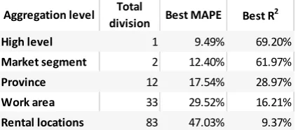
SQ3. What aggregation level works best for the demand prediction?

Several possible aspects for aggregation level for a demand prediction model were found through literature study. Among them, the time interval, product type and spatial aggregation are the most relevant to our study. For the time interval, we used daily aggregate of the data as required for the planning activity that becomes the focus of our research. For the product type and spatial level, demand prediction models were built and compared for various aggregation levels. For product type, two demand prediction models for B2B and B2C market segments were developed. The evaluation shows that the performance of the demand prediction per market segment are lower than the high-level prediction (i.e. aggregated segment), with the mean average percentage error of 12.4% and 14.8% for B2C and B2B segment respectively, compared to 9.49% MAPE for the aggregated segment. For spatial aggregation, three deeper aggregation levels were considered, which are province, work area, and rental locations. Each of this level has a varying number of area and there are diverse ranges of demand values for every area which lead to varying performances per area. Table 1 shows the best performance out of all divisions within each aggregation level.

Table 1 Summary of the best performance of different aggregation level models

We found that the higher the granularity, the less satisfactory the prediction performance is. For the low-level prediction with relatively low average demand, the models tend to predict around the average demand value. For some area, the R2 _{scores even suggest that the models perform worse}

than predictions using the average value. This condition is found in all the spatial aggregation levels considered. Therefore, it is clear that for predictions with daily time interval, the aggregation level that works best is the highest level, which is all demand in the Netherlands for all market segment. The second best would be the predictions per market segment since it exhibits an acceptable performance while offering more detailed information for operational planning.

SQ4. How can we estimate uncertainty of the prediction result?

Prediction interval is widely suggested in literature as a means of presenting uncertainty. We compared three techniques to provide lower and upper bound of the daily demand prediction: using constant variance from the prediction model, variance of a fitted error model (both assuming observations are normally distributed) and quantile regression. We measured the performance of each approach based on the prediction interval coverage probability (PICP) and mean prediction interval width (MPIW). There is a clear trade-off between PICP and MPIW demonstrated in the performance of all prediction interval techniques. The constant variance approach results in the highest coverage compared to the others, in fact 95.82%, followed by quantile regression with 90.783%, and error model with 88.52%. However, the error model approach produced the most reasonable result in terms of the MPIW. Among the three approaches, the error model and quantile regression approaches offer more information compared to the constant variance. The variations in interval width from day to day produced in the two non-constant approach may indicate when prediction is less reliable as a wider interval implies a higher uncertainty. Furthermore, as we found that high uncertainty does not always mean a high error, we proposed an outlier separation and

Aggregation level Total

division Best MAPE Best R

2

High level 1 9.49% 69.20%

Market segment 2 12.40% 61.97%

Province 12 17.54% 28.97%

Work area 33 29.52% 16.21%

19 classification approach that can be utilized as an indicator of the days on which the error of the prediction is expected to be high, hence suggesting the need of forecasters to intervene with the results.

Finally, we can conclude the answer to the main research questions as follows.

RQ: To what extent can we predict the demand of replacement cars in the Netherlands?

By using regression models and framing the time series problem as a supervised learning problem, we can generate a prediction for the daily demand of replacement cars in the Netherlands. Historical data and external data like weather and calendar data are proven to be useful for the demand prediction. The best performing model can predict the demand of replacement cars per day with 9.49% average percentage error in the country level. The distribution of the error for has shown that the model performed decently for almost 80% of the cases but it has high errors for the remaining cases. In fact, based on the proposed outlier analysis, the exclusion of the outliers has resulted in a 5.89% average percentage error.

The performance of the demand prediction gradually decreases each time we add more granularity to the prediction (i.e. predicting at lower aggregation level). For prediction per market segment at country level, the performance seems to be acceptable despite the decrease from the performance of the highest level. For province level, some provinces still demonstrate acceptable performances, but the less busy provinces suggest differently. The same goes for the even deeper work area and rental locations level. For this granularity, we found at some area resembles that of an intermittent demand, which the current input features and machine learning approach cannot predict effectively.

Moreover, in terms of the explained variance, the input features in the best performing model can explain up to 69% variance in the demand value. However, it still has a considerable percentage of unexplained variance, in fact 31%, which shows that the case has a significant random effect and/or there are other important predictors that cannot or has yet been incorporated in our model that can improve the performance of the model. According to the different approach that we implemented to generate the prediction interval, this performance of 9.49% error and 69% explained variance have an uncertainty where the half width of the interval in average is at least two times the average error of the prediction. To sum up, it is not possible to predict the demand of the replacement cars completely accurately. However, with the support of knowledge from the domain experts, supplementary components to the prediction like prediction interval and outlier analysis can be effectively used to enhance the demand prediction.

8.2

C

This research contributed to an enhancement of the current knowledge on the existing literature on rental cars demand prediction and demand prediction using machine learning techniques in general. This has been achieved by empirically testing a number of prediction models on a real-life dataset. This study provides valuable knowledge on what factors are important to predict the demand of replacement cars on a daily level. To the best of our knowledge, no literature has explored this topic for the specific domain application.

20 category/characteristics (i.e. parametric, non-parametric, supervised learning on residuals), which can be generally applied to a wide variety of machine learning models. Previous research for demand forecasting using machine learning tend to focus on providing only the point forecast, while some others focus on proposing methods to generate prediction interval on top of a specific algorithm.

In this study, we have also directly compared and discussed the effect of deeper location level or more granular spatial aggregation. As far as we can tell, most research focused on investigating the different time aggregation for the prediction period or time window. Little has explicitly analyzed the effect of various location aggregation level in predicting time series demand.

21

R

EFERENCES

[1] Aburto, L., & Weber, R. (2007). Improved supply chain management based on hybrid demand forecasts. Applied Soft Computing, 7(1), 136-144.

[2] Aguinis, H., Gottfredson, R. K., & Joo, H. (2013). Best-Practice Recommendations for Defining, Identifying, and Handling Outliers. Organizational Research Methods, 16(2), 270–301. doi:10.1177/1094428112470848

[3] Allstate Roadside Services. (2019). Data & Analytics, the future of roadside is here. Retrieved July 12, 2019, from https://www.allstateroadsideservices.com/roadside-solutions/data-analytics.aspx

[4] Ampazis, N. (2015). Forecasting Demand in Supply Chain Using Machine Learning Algorithms. International Journal of Artificial Life Research (IJALR), 5(1), 56-73.

[5] Antunes, A., Andrade-Campos, A., Sardinha-Lourenço, A., & Oliveira, M. S. (2018). Short-term water demand forecasting using machine learning techniques. Journal of Hydroinformatics, 20(6), 1343-1366.

[6] ANWB. (2019, July 04). Pechhulp van de Wegenwacht: ANWB Wegenwacht®. Retrieved July 12, 2019, from https://www.anwb.nl/wegenwacht

[7] ANWB. (2019, January 28). The Royal Dutch Touring Club ANWB. Retrieved July 13, 2019, from https://www.anwb.nl/over-anwb/vereniging-en-bedrijf/organisatie/english-page

[8] Arlot, S., & Celisse, A. (2010). A survey of cross-validation procedures for model selection. Statistics

surveys, 4, 40-79.

[9] Bergmeir, C., & Benítez, J. M. (2012). On the use of cross-validation for time series predictor evaluation. Information Sciences, 191, 192-213. Bishop, C. (1991). Improving the generalization properties of radial basis function neural networks. Neural computation, 3(4), 579-588.

[10]Bishop, C. M. (2006). Pattern recognition and machine learning. springer.

[11]Böse, J. H., Flunkert, V., Gasthaus, J., Januschowski, T., Lange, D., Salinas, D., ... & Wang, Y. (2017). Probabilistic demand forecasting at scale. Proceedings of the VLDB Endowment, 10(12), 1694-1705. [12]Bontempi, G., Taieb, S. B., & Le Borgne, Y. A. (2012, July). Machine learning strategies for time series

forecasting. In European business intelligence summer school (pp. 62-77). Springer, Berlin, Heidelberg. [13]Botchkarev, A. (2018). Performance Metrics (Error Measures) in Machine Learning Regression,

Forecasting and Prognostics: Properties and Typology. arXiv preprint arXiv:1809.03006.

[14]Brando, A., Rodríguez-Serrano, J. A., Ciprian, M., Maestre, R., & Vitrià, J. (2018, September). Uncertainty Modelling in Deep Networks: Forecasting Short and Noisy Series. In Joint European

Conference on Machine Learning and Knowledge Discovery in Databases (pp. 325-340). Springer,

Cham.

[15]Brochu, E., Cora, V. M., & De Freitas, N. (2010). A tutorial on Bayesian optimization of expensive cost functions, with application to active user modeling and hierarchical reinforcement learning. arXiv

preprint arXiv:1012.2599.

[16]Burrough, P. A., McDonnell, R., McDonnell, R. A., & Lloyd, C. D. (2015). Principles of geographical information systems. Oxford university press.

[17]Cankurt, S., & Subasi, A. (2015). Developing tourism demand forecasting models using machine learning techniques with trend, seasonal, and cyclic components. Balkan Journal of Electrical and

Computer Engineering, 3(1), 42-49.

22 [19]Carbonneau, R., Laframboise, K., & Vahidov, R. (2008). Application of machine learning techniques for

supply chain demand forecasting. European Journal of Operational Research, 184(3), 1140-1154. [20]Chapman, P., Clinton, J., Kerber, R., Khabaza, T., Reinartz, T., Shearer, C., & Wirth, R. (2000). CRISP-DM

1.0 Step-by-step data mining guide.

[21]Chatfield, C. (1993). Calculating interval forecasts. Journal of Business & Economic Statistics, 11(2), 121-135.

[22]Chen, K. Y., & Wang, C. H. (2007). Support vector regression with genetic algorithms in forecasting tourism demand. Tourism Management, 28(1), 215-226. das Chagas Moura, M., Zio, E., Lins, I. D., & Droguett, E. (2011). Failure and reliability prediction by support vector machines regression of time series data. Reliability Engineering & System Safety, 96(11), 1527-1534.

[23]DiCicco‐Bloom, B., & Crabtree, B. F. (2006). The qualitative research interview. Medical

education, 40(4), 314-321.

[24]Domingos, P. M. (2012). A few useful things to know about machine learning. Commun. acm, 55(10), 78-87.

[25]Dosser, M. (2016, December 13). ÖAMTC Mitgliedschaft. Retrieved July 12, 2019, from https://www.oeamtc.at/mitgliedschaft/

[26]Ericsson, N. R. (2001). Forecast uncertainty in economic modeling. FRB International Finance Discussion Paper, (697). Board of Governors of the Federal Reserve System (U.S.).

[27]Fink, A., & Reiners, T. (2006). Modeling and solving the short-term car rental logistics problem. Transportation Research Part E: Logistics and Transportation Review, 42(4), 272-292. [28]Geraghty, M. K., & Johnson, E. (1997). Revenue management saves national car

rental. Interfaces, 27(1), 107-127.

[29]Gopi, G., Dauwels, J., Asif, M. T., Ashwin, S., Mitrovic, N., Rasheed, U., & Jaillet, P. (2013, October). Bayesian support vector regression for traffic speed prediction with error bars. In 16th International

IEEE Conference on Intelligent Transportation Systems (ITSC 2013) (pp. 136-141). IEEE.

[30]Green Flag. (2019). Breakdown cover, assistance and recovery, whenever you need us: Green Flag. Retrieved July 12, 2019, from https://www.greenflag.com/breakdown-cover

[31]Gupta, M., Gao, J., Aggarwal, C. C., & Han, J. (2014). Outlier detection for temporal data: A survey. IEEE Transactions on Knowledge and Data Engineering, 26(9), 2250-2267.

[32]Gupta, R., & Pathak, C. (2014). A machine learning framework for predicting purchase by online customers based on dynamic pricing. Procedia Computer Science, 36, 599-605.

[33]Hall, M. A. (2000). Correlation-based feature selection of discrete and numeric class machine learning. [34]Hansen, B. E. (2006). Interval forecasts and parameter uncertainty. Journal of Econometrics, 135(1-2),

377-398.

[35]Herrera, M., Torgo, L., Izquierdo, J., & Pérez-García, R. (2010). Predictive models for forecasting hourly urban water demand. Journal of hydrology, 387(1-2), 141-150.

[36]Hong, W. C., Lai, Y. J., Pai, P. F., Lee, S. L., & Yang, S. L. (2007, September). Composite of support vector regression and evolutionary algorithms in car-rental revenue forecasting. In 2007 IEEE Congress on Evolutionary Computation (pp. 2872-2878). IEEE.

[37]Hyndman, R. J. (2006). Another look at forecast-accuracy metrics for intermittent demand. Foresight: The International Journal of Applied Forecasting, 4(4), 43-46.

23 [39]Jackson, B. (2018, September 27). AI-powered CAA roadside assistance will be dispatched before you break down. Retrieved July 12, 2019, from https://www.itworldcanada.com/article/ai-powered-caa-roadside-assistance-will-be-dispatched-before-you-break-down/409330

[40]Kandasamy, K., Vysyaraju, K. R., Neiswanger, W., Paria, B., Collins, C. R., Schneider, J., ... & Xing, E. P. (2019). Tuning Hyperparameters without Grad Students: Scalable and Robust Bayesian Optimisation with Dragonfly. arXiv preprint arXiv:1903.06694.

[41]Kharfan, M., & Chan, V. W. (2018). Forecasting Seasonal Footwear Demand Using Machine Learning (Master's thesis, Massachusetts Institute of Technology, 2018). Cambridge: MIT. Retrieved from https://dspace.mit.edu/.

[42]Kim, S., & Kim, H. (2016). A new metric of absolute percentage error for intermittent demand forecasts. International Journal of Forecasting, 32(3), 669-679.

[43]Knuth, D. E. (1992). Literate Programming. Number 27 in CSLI Lecture Notes. Center for the Study of

Language and Information, 349-358.

[44]Kotsiantis, S. B., Kanellopoulos, D., & Pintelas, P. E. (2006). Data preprocessing for supervised leaning. International Journal of Computer Science, 1(2), 111-117.

[45]Kvålseth, T. O. (1985). Cautionary note about R 2. The American Statistician, 39(4), 279-285.

[46]Laurikkala, J., Juhola, M., Kentala, E., Lavrac, N., Miksch, S., & Kavsek, B. (2000, August). Informal identification of outliers in medical data. In Fifth international workshop on intelligent data analysis in medicine and pharmacology (Vol. 1, pp. 20-24).

[47]Lei, S., Wang, H., Yang, C., Du, B., Zhong, R., & Huang, R. (2017, August). Forecasting car rental demand based temporal and spatial travel patterns. In 2017 IEEE SmartWorld, Ubiquitous Intelligence & Computing, Advanced & Trusted Computed, Scalable Computing & Communications, Cloud & Big

Data Computing, Internet of People and Smart City Innovation

(SmartWorld/SCALCOM/UIC/ATC/CBDCom/IOP/SCI) (pp. 1-8). IEEE.

[48]Liu, C. B., Chamberlain, B. P., Little, D. A., & Cardoso, Â. (2017, September). Generalising random forest parameter optimisation to include stability and cost. In Joint European Conference on Machine

Learning and Knowledge Discovery in Databases (pp. 102-113). Springer, Cham.

[49]Luo, G. (2016). A review of automatic selection methods for machine learning algorithms and hyper-parameter values. Network Modeling Analysis in Health Informatics and Bioinformatics, 5(1), 18. [50]Makridakis, S., Spiliotis, E., & Assimakopoulos, V. (2018). Statistical and Machine Learning forecasting

methods: Concerns and ways forward. PloS one, 13(3), e0194889.

[51]Mayr, A., Hothorn, T., & Fenske, N. (2012). Prediction intervals for future BMI values of individual children-a non-parametric approach by quantile boosting. BMC Medical Research Methodology, 12(1), 6.

[52]McKay, M. D. (1995). Evaluating prediction uncertainty (No. NUREG/CR--6311). Nuclear Regulatory Commission.

[53]Mupparaju, K., Soni, A., Gujela, P., & Lanham, M.A. (2018). A Comparative Study of Machine Learning Frameworks for Demand Forecasting.

[54]Murphy, A. H. (1993). What is a good forecast? An essay on the nature of goodness in weather forecasting. Weather and forecasting, 8(2), 281-293.

[55]Neter, J., Kutner, M. H., Nachtsheim, C. J., & Wasserman, W. (1996). Applied linear statistical models (Vol. 4, p. 318). Chicago: Irwin.

[56]O’Donnell, A. R. (2014, November 19). Agero Introduces Enhanced Analytics to Support Roadside

24 [57]Oliveira, B. B., Carravilla, M. A., & Oliveira, J. F. (2017a). Fleet and revenue management in car rental

companies: A literature review and an integrated conceptual framework. Omega, 71, 11–26.

[58]Oliveira, B. B., Carravilla, M. A., & Oliveira, J. F. (2017b, June). A Dynamic Programming Approach for Integrating Dynamic Pricing and Capacity Decisions in a Rental Context. In Congress of APDIO, the

Portuguese Operational Research Society (pp. 297-311). Springer, Cham.

[59]Pachon, J., Iakovou, E., & Chi, I. (2006). Vehicle fleet planning in the car rental industry. Journal of

Revenue and Pricing Management, 5(3), 221-236.

[60]Palshikar, G. (2009, June). Simple algorithms for peak detection in time-series. In Proc. 1st Int. Conf. Advanced Data Analysis, Business Analytics and Intelligence (Vol. 122).

[61]Pedregosa, F., Varoquaux, G., Gramfort, A., Michel, V., Thirion, B., Grisel, O., ... & Vanderplas, J. (2011). Scikit-learn: Machine learning in Python. Journal of machine learning research, 12(Oct), 2825-2830.

[62]Petropoulos, F., Makridakis, S., Assimakopoulos, V., & Nikolopoulos, K. (2014). ‘Horses for Courses’ in

demand forecasting. European Journal of Operational Research, 237(1), 152-163.

[63]Pinson, P. (2012). Very‐short‐term probabilistic forecasting of wind power with generalized logit–

normal distributions. Journal of the Royal Statistical Society: Series C (Applied Statistics), 61(4), 555-576.

[64]Prytz, R. (2014). Machine learning methods for vehicle predictive maintenance using off-board and on-board data (Doctoral dissertation, Halmstad University Press).

[65]Qiu, X., Zhang, L., Ren, Y., Suganthan, P. N., & Amaratunga, G. (2014, December). Ensemble deep learning for regression and time series forecasting. In 2014 IEEE symposium on computational

intelligence in ensemble learning (CIEL) (pp. 1-6). IEEE.

[66]RAC. (2019). Breakdown cover. Retrieved July 12, 2019, from https://www.rac.co.uk/breakdown-cover

[67]Roy, D., Pazour, J. A., & De Koster, R. (2014). A novel approach for designing rental vehicle repositioning strategies. IIE Transactions, 46(9), 948-967.

[68]Ru, B., McLeod, M., Granziol, D., & Osborne, M. A. (2017). Fast information-theoretic Bayesian optimisation. arXiv preprint arXiv:1711.00673.

[69]Shahrabi, J., Mousavi, S. S., & Heydar, M. (2009). Supply chain demand forecasting: A comparison of machine learning techniques and traditional methods. Journal of Applied Sciences, 9(3), 521-527. [70]Shearer, C. (2000). The CRISP-DM model: the new blueprint for data mining. Journal of data

warehousing, 5(4), 13-22.

[71]Snoek et al. Snoek, J., Larochelle, H., & Adams, R. P. (2012). Practical bayesian optimization of machine learning algorithms. In Advances in neural information processing systems (pp. 2951-2959). [72]Somasundaram, R. S., & Nedunchezhian, R. (2011). Evaluation of three simple imputation methods for

enhancing preprocessing of data with missing values. International Journal of Computer Applications, 21(10), 14-19.

[73]Taieb, S. B., Huser, R., Hyndman, R. J., & Genton, M. G. (2016). Forecasting uncertainty in electricity smart meter data by boosting additive quantile regression. IEEE Transactions on Smart Grid, 7(5), 2448-2455.

[74]Taylor, S. J., & Letham, B. (2018). Forecasting at scale. The American Statistician, 72(1), 37-45.

[75]Tugay, R., & Ögüdücü, S. G. (2017). Demand Prediction using Machine Learning Methods and Stacked Generalization. In Proceedings of the 6th International Conference on Data Science, Technology and

25 [76]van der Spoel, S., Amrit, C. A., & van Hillegersberg, J. (2016, March). The role of domain analysis in prediction instrument development. In Big Data Interoperability for Enterprises (BDI4E) Workshop

2016.

[77]van Hinsbergen, C. I., Van Lint, J. W. C., & Van Zuylen, H. J. (2009). Bayesian committee of neural networks to predict travel times with confidence intervals. Transportation Research Part C: Emerging

Technologies, 17(5),

[78]Verma, M., Gangadharan, G. R., Narendra, N. C., Vadlamani, R., Inamdar, V., Ramachandran, L., Calheiros, R. N. & Buyya, R. (2016). Dynamic resource demand prediction and allocation in multi‐

tenant service clouds. Concurrency and Computation: Practice and Experience, 28(17), 4429-4442. [79]Weinberger, K., Dasgupta, A., Attenberg, J., Langford, J., & Smola, A. (2009). Feature hashing for large

scale multitask learning. arXiv preprint arXiv:0902.2206.

[80]Whitt, W., & Zhang, X. (2019). Forecasting arrivals and occupancy levels in an emergency department. Operations Research for Health Care.

[81]Wijaya, T. K., Sinn, M., & Chen, B. (2015, April). Forecasting uncertainty in electricity demand.

In Workshops at the Twenty-Ninth AAAI Conference on Artificial Intelligence.

[82]Xu, J. X., & Lim, J. S. (2007, September). A new evolutionary neural network for forecasting net flow of a car sharing system. In 2007 IEEE Congress on Evolutionary Computation(pp. 1670-1676). IEEE. [83]Yang, Y., Jin, W., & Hao, X. (2008, October). Car rental logistics problem: a review of literature. In 2008

IEEE International Conference on Service Operations and Logistics, and Informatics (Vol. 2, pp.

2815-2819). IEEE.

[84]Zhang, G. P. (2003). Time series forecasting using a hybrid ARIMA and neural network model. Neurocomputing, 50, 159-175.

[85]Zhou, Q., Han, R., & Li, T. (2015, December). A two-step dynamic inventory forecasting model for large manufacturing. In 2015 IEEE 14th International Conference on Machine Learning and Applications

(ICMLA) (pp. 749-753). IEEE.