Research and development of ground based transiting extrasolar planet projects

(1)

University of Warwick institutional repository:

http://go.warwick.ac.uk/wrap

A Thesis Submitted for the Degree of PhD at the University of Warwick

http://go.warwick.ac.uk/wrap/54441

This thesis is made available online and is protected by original copyright.

Please scroll down to view the document itself.

(2)

Research and development of ground-based

transiting extrasolar planet projects

by

Jo˜

ao Paulo da Silva Bento

Thesis

Submitted to the University of Warwick

for the degree of

Doctor of Philosophy

Department of Physics

(3)

List of Tables

3.1 Selection parameters for ULTRACAM observations . . . 104 3.2 ULTRACAM Observations of large scale-height planets . . . 112 3.3 Magnitude and color of WASP-15, WASP-17 and comparisons . . . . 114 3.4 Extinction coefficients for the WASP-15 observation of 2010-04-25 . 124 3.5 Extinction coefficients for the WASP-17 observation of 2010-04-26 . 124 3.6 Initial system parameters for WASP-17 . . . 144

(7)

List of Figures

1.1 Exoplanet Detections for all methods . . . 3

1.2 Direct imaging of exoplanets . . . 5

1.3 Expected astrometric signatures of known planets . . . 7

1.4 Radial velocity of 51 Peg b . . . 8

1.5 Radial velocity of HD156846b . . . 9

1.6 Microlensing events . . . 13

1.7 Transit light curve of HD209458b . . . 14

1.8 Schematics of transiting planet . . . 15

1.9 Transits of HD209458b using HST . . . 17

1.10 The SuperWASP Instrument . . . 21

1.11 SuperWASP Passband responce . . . 22

1.12 Kepler light curve of planet Kepler-4b . . . 28

1.13 Kepler light curve of planet Kepler-16b . . . 29

1.14 NGTS parameter space of optimal sensitivity . . . 33

1.15 NGTS prototype data quality . . . 35

1.16 CCD readout analogy with buckets . . . 37

1.17 Saturated star example . . . 38

1.18 Schematic Figure demonstrating transmission spectroscopy . . . 43

1.20 Spitzer secondary eclipses of WASP-18b . . . 46

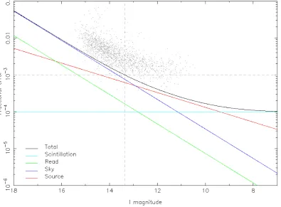
2.1 SuperWASP noise model . . . 54

2.2 Fractional RMS vs magnitude for SuperWASP 2007 data . . . 56

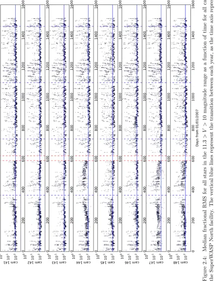
2.4 Median fractional RMS for SuperWASP North . . . 60

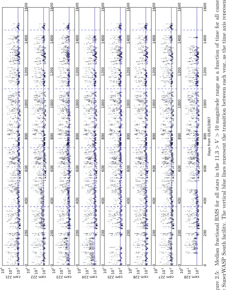
2.5 Median fractional RMS for SuperWASP South . . . 61

2.6 SuperWASP camera 141 Detector map . . . 65

(8)

2.8 Plots displaying the typical results of SuperWASP gradient removal 69

2.9 Selected enlarged regions of detector map and twilight flat . . . 73

2.10 More selected enlarged regions of detector map and twilight flat . . . 75

2.11 Bad column vertical profiles for several illumination levels . . . 76

2.12 12 night evolution of twilight flats . . . 78

2.13 12 night evolution of sky flats . . . 78

2.14 Plot representation of a detector map feature . . . 80

2.15 Another plot representation of a detector map feature . . . 81

2.16 Full moon and dark night results of twilight flat fielding . . . 82

2.17 Enlarged section of the CCD under several analysis processes . . . . 83

2.18 Detector map evolution for camera 141 . . . 86

2.19 Detector map evolution for camera 147 . . . 87

2.20 Fractional RMS vs magnitude for SuperWASP 2009 data with detec-tor map series . . . 89

2.22 Fractional RMS vs magnitude for SuperWASP 2011 data with detec-tor map series . . . 91

2.23 Fractional RMS vs magnitude for SuperWASP 2011 data with detec-tor map series. Histograms with improvement analysis . . . 93

3.1 Exoplanet transmission spectra for two classes with ULTRACAM filters 97 3.2 ULTRACAM photo and schematic . . . 99

3.3 ULTRACAM filter responses . . . 100

3.4 Pictorial representation of the planetary scale height . . . 102

3.5 Results from an optimal defocus study for airmass 2 . . . 107

3.6 Results from an optimal defocus study for airmass 1 . . . 108

3.7 Results from an optimal defocus study for high sky brightness . . . . 110

3.8 Finding charts for WASP-15 and WASP-17 . . . 113

3.9 Example ULTRACAM frames for WASP-15 and WASP-17 . . . 113

3.10 ULTRACAM r’ band raw flux photometry of comparison star of WASP-15 . . . 116

3.11 Graphical representation of airmass . . . 117

3.12 Airmass corrections for the WASP-15b transit observation . . . 119

3.13 Raw fluxes for WASP-15 observation on 2010-04-25 . . . 121

3.14 Raw fluxes for WASP-15 observation on 2010-05-10 . . . 122

(9)

3.17 Background levels for WASP-15 observation on 2010-04-25 in the g

band . . . 127

3.18 Background subtraction test . . . 129

3.19 Aperture positions for WASP-15b observation of 2010-04-25 . . . 130

3.20 Flat field correlation test for WASP-15’s comparison star 1 . . . 133

3.21 Flat field correlation test for WASP-15’s comparison star 2 . . . 134

3.22 Raw flux as a function of parallactic angle for comparison star 1 . . 135

3.23 Visual result of guide probe vignetting test . . . 137

3.24 Visual result of guide probe vignetting test in position 3 . . . 140

3.25 Visual result of guide probe vignetting test in position 6 . . . 141

3.26 Average of 200 rows of the result of the guide probe test . . . 142

3.27 Di↵erential photometry curves for the WASP-17b observation of 2010-04-26 with model light curve . . . 146

3.28 Di↵erential photometry curves for the WASP-17b observation of 2010-04-26 fitted for planetary radius . . . 147

3.29 Planet radius as function of wavelength for WASP-17b . . . 148

4.1 Sky coverage of the SuperWASP project . . . 152

4.2 Mass-Period distribution of close-in exoplanets . . . 154

4.3 Fraction of available nights at La Silla and Paranal . . . 157

4.4 Performance of a model of the brightness of Moonlight . . . 160

4.5 Sky coverage for the NGTS instrument . . . 165

4.6 Sky coverage for the SuperWASP instrument . . . 168

4.7 Planet detection probability software outcome . . . 173

4.8 Probability of planetary detection as a function of maximum zenith distance . . . 175

4.9 Probability of planetary detection for di↵erent locations . . . 177

(10)

Acknowledgments

I am profoundly grateful to Dr. Peter Wheatley for all his guidance, patience

and support throughout my PhD. I would like to thank the University of Warwick

Astronomy and Astrophysics Group for making me feel truly at home and Dr.

Richard West for maintaining the SuperWASP archive and for being generally a

constant source of invaluable help.

A huge thanks goes to a remarkable group of friends who have made the last

three years the best of my life (so far). In particular, I would like to thank Simon,

Jon, Steve, Lieke, Rachel and Dave for playing a massive part in that, being the best

friends anyone could hope to have, and for allowing me to be myself without (too

many) questions asked. I gratefully salute the Motorcade crew for all the wonderful

times and for giving me the chance to fulfil a life-long dream. A special thanks

goes out to Steel Panther, for providing the perfect soundtrack and for being simply

awesome.

None of this work would have been possible, of course, without the constant

love and support of my family. They have provided me with much needed help and

a range of opportunities, for which I am eternally grateful. They have been the

foundations of all my achievements and their unending belief and encouragement

(11)

Declarations

I declare that the work presented in this thesis is my own except where

stated otherwise, and was carried out entirely at the University of Warwick, during

the period October 2008 to May 2012, under the supervision of Dr. Peter Wheatley.

The research reported here has not been submitted, either wholly or in part, in this

or any other academic institution for admission to a higher degree.

Conference contributions based on this thesis are:

• National Astronomy Meeting, Glasgow, UK, April 2010, Poster presentation:

Finding smaller planets with SuperWASP.

• SuperWASP consortium meeting, St. Andrews, UK, September 2010, Oral presentation: SuperWASP detector map analysis.

(12)

Abstract

The search for exoplanets has gone from the realm of speculation to being one of the most prolific topics of modern astronomy in the space of just 20 years. In particular, the geometric alignment of transiting exoplanets provides the added opportunity to measure a host of properties of these systems, including studies of planetary atmospheres.

The vast majority of known transiting exoplanets to date were found using dedicated ground-based surveys such as the SuperWASP project. Such enterprises comprise of multiple small telescopes designed to perform high-precision photome-try over a wide field of view and rely on efficiently compensating for several noise contributions. An analysis of the sources of noise in the SuperWASP light curves was performed, focussing on systematic e↵ects fixed in detector space. A study of a set ofdetector maps produced from the average of the fractional residuals of the light curves in CCD coordinates has revealed that the current flat-fielding strategy is introducing a component of red noise into the light curves due to the wavelength-dependent nature of the CCDs. The possibility of using such maps as a basis for an additional decorrelation step in the software pipeline is discussed.

The next phase in planetary discoveries from ground-based surveys consists of the search for smaller planets and those in longer orbits around their host stars. This process involves an observing strategy that focuses on intensive coverage of particular locations of the sky. We develop simulation software to aid the choice of observed fields for the SuperWASP and Next Generation Transit Survey (NGTS) projects in order to maximise the chances of finding planets at those locations. Moreover, this simulation can be used for comparative studies of the planet finding probability for several design choices and has been used to justify the necessity to commission the NGTS instrument at ESO’s Paranal Observatory in order to benefit from one of the World’s premier sites.

(13)

Abbreviations

QE Quantum Efficiency

CCD Charged Coupled Devices

S/N Signal-to-noise

NaN Not a Number

ADU Analog/Digital Unit

FWHM Full Width Half Maximum

RMS Root Mean Squared

AU Astronomical Unit

PSF Point Spread Function

Alt/Az Altazimuth mount

FOV Field of view

MJ Jupiter Mass

RJ Jupiter Radius

RV Radial Velocity

NTT New Technology Telescope

WHT William Herschel Telescope

WASP Wide Angle Search for Planets

NGTS Next Generation Transit Survey

HST Hubble Space Telescope

ESO European Southern Observatory

ESA European Space Agency

NASA National Aeronautics and Space

(14)

Chapter 1

Introduction

1.1 Exoplanets

The word exoplanet simply means extrasolar planet, which refers to any planet found outside of our Solar System. The existence of such bodies was part of the realm of speculation until 1992, when 3 terrestrial-mass planets were found orbiting the pulsar PSR B1257+12 [Wolszczan & Frail, 1992]. These planets cause a reflex motion on the orbit of the star which lead to the apparent change in the pulsar’s rotational frequency as the pulses seem to arrive faster when the star is moving towards the observer and vice-versa. The first discovery of an exoplanet orbiting a main-sequence star came only three years after, when a Jupiter mass body was found to orbit the star 51 Peg [Mayor & Queloz, 1995]. In this case, variations of the radial velocity of the star with respect to the Sun were detected, and the presence of the planet inferred (see Section 1.2 for more details on this method). This discovery was the trigger for a change in the mindset of the astronomical community, where the study of exoplanets is now a major field of scientific research. Many of the planets known today fall under the category ofhot Jupiters, which are Jupiter mass planets orbiting very close to their parent stars, typically at separations under 0.1AU. The definition is loose and several authors have defined a sub-set of these as very hot Jupiters if the orbital period is under 3 days [Beatty & Gaudi, 2008] or the separation is under 0.025AU [Ragozzine & Wolf, 2009]. However, a whole host of smaller examples are being found on a regular basis1_{, with} _⇡ _33% of known planets having masses lower than that of Saturn. The dominance of hot Jupiters comes from the observational bias of current instruments. Massive planets close to their host stars are typically much easier to find than small bodies at large

(15)

separations.

The numbers of known planets, within 20 years of the discovery of the first sub-stellar body outside our Solar System, have risen to close to a thousand. We are entering a new age of exoplanet exploration, where such numbers allow us to perform reliable and meaningful statistics, such as those performed recently by Mayor et al. [2011] or by Wolfgang & Laughlin [2011]. The time has also come to further study the properties of these bodies in more detail. Section 1.5.4 contains an introduction to a potential example of such studies. Throughout this thesis, and indeed in the field of exoplanets in general, the naming convention for any planet outside the Solar System consists of adding a lower case letter to the host star’s denomination for each planet, starting with b, in order of discovery. For example, if the star is namedWASP-1, the first planet to be discovered orbiting it will be named WASP-1b, the secondWASP-1c and so on.

1.2 Detection methods

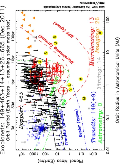
Finding exoplanets is challenging due to the very high contrast between the reflected light from the planet and the stellar emission and the relatively small sep-aration between both. It is therefore extremely hard to image these objects directly, and often astronomers rely on measuring the impact of the planet on its host star. Figure 1.1 shows a plot of the mass as a function of the orbital separation for all con-firmed planets discovered by December 2011 (courtesy of Keith Horne). This Figure shows that the majority of planets have been found by radial velocity measurements (namedDoppler in the Figure), but transiting planets also have contributed consid-erably to the numbers of known planets. Moreover, direct imaging is responsible for the vast majority of planets at large orbital separations, whereas the microlensing technique yields results with planet masses as low as a few Earth masses, but re-stricted to a relatively small range of orbital separations. These observational biases are addressed in more detail as each method is explored.

The following Sections describe the most commonly used detection methods of exoplanets to date. Transiting planets are described in more detail in Section 1.3.

1.2.1 Direct Imaging

(16)

[image:16.595.89.481.152.691.2]

(17)

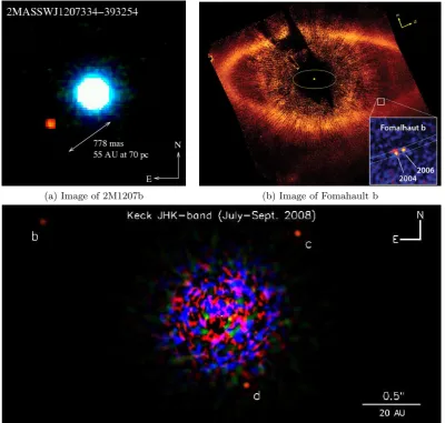
ential imaging coupled with adaptive optics [Marois et al., 2008]. There is therefore a bias towards young massive planets, since these still have temperatures higher than the equilibrium temperature due to stellar irradiation, thereby exhibiting high thermal emission. This technique is also more sensitive to planets on long orbits (separations of 8-200 AU), as the large separation will help with the limited res-olution of the current telescopes. This is evident in Figure 1.1, since the planets detected by direct imaging dominate the higher orbital separation region on the plot. The large periods of these systems and the associated difficulty in directly observing the planet moving around the star on feasible time-scales makes it harder to distinguish these planetary companions from background objects at short angular separations from the target star. This is done by ensuring that the two objects form a common proper-motion pair [Seager, 2010b, Part II].

In the first of these discoveries it was possible to image a 5 MJplanet directly [Chauvin et al., 2004] with the use of adaptive optics. 2M1207 is a nearby young brown dwarf, located at approximately 70 pc from the Sun, and its companion orbits at around 55AU from the host star. Therefore, the combined inherent faintness of the host star, proximity, age and large separation between the two bodies has made this discovery possible. Figure 1.2a contains the obtained image for this system.

(18)

(a) Image of 2M1207b (b) Image of Fomahault b

[image:18.595.121.522.175.556.2]

(c) Image of the HR8799 system

(19)

(d < 5pc). Hence, there is an observational bias towards imaging known planets, young stellar systems and nearby stars.

1.2.2 Reflex motion of the star

This subsection describes a series of methods that rely on the fact that a planet and its host star both orbit a common centre of mass. The relative position of any star with respect to an observer on Earth is mostly dictated by its motion within the galaxy, the orbit of the Solar System in the galaxy and the orbital speed of the Earth around the Sun. It is often the case that the orbits of stars in the galaxy are defined with respect to the Local Standard of Rest (LSR). This, in turn, is defined as the rotational velocity for a circular orbit in the galactic plane. The motion of the stars in the galaxy is, however, distinctly non-Keplerian due to the nonspherical mass distribution within the galaxy. Nevertheless, they are often stable and the Earth’s orbit can be accounted for easily in the context of a heliocentric correction. Therefore, if any periodic perturbations to the motion of another star are detected it is possible to infer the presence of additional bodies in the system.

Astrometry

This technique consists of measuring the relative positions of a particular star and look for variations with respect to other objects in the sky. Specifically, it relies on a measurement of the second-order perturbation (wobble) of the position of the star with respect to background sources, only noticeable after other larger components, such as proper motion and parallax, have been accounted for. This method is therefore optimised for nearby stars and limited by the resolution of the telescopes used. The motion of a star orbiting the centre of mass of a star-planet system as an eclipse with angular semi-major axis↵ is given by

↵= ✓_M

p

M_⇤

◆ ✓ _a

1AU ◆ ✓ _d

1pc ◆ 1

arcsec, (1.1)

assuming the mass of the planetMp is much smaller than the mass of the star M⇤

[Perryman, 2011]. In this equation, d is the distance to the system and a is the semi-major axis of the orbit (assumed circular).

(20)

[image:20.595.230.415.112.296.2]

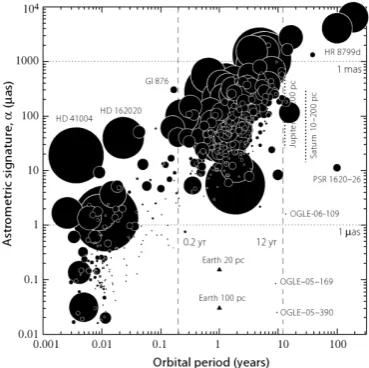
Figure 1.3: Astrometric signature,↵, as a function of period calculated for known planetary systems using equation 1.1. The sizes of the circles correspond to Mp

or Mpsini, depending on whether the degeneracy has been solved using several

detection methods. Horizontal lines show the 1mas and 1µas levels. For comparison, the signatures of Solar System planets at relevant distances is also depicted. From Perryman [2011].

of known planets are expected to yield a signature of under 1mas in amplitude. An astrometric measurement was made with HST by Benedict et al. [2002] of previously known planet Gliese 876b and, despite the fact that a non-negligible number of false positives have been suggested in the past, the upcoming ESA mission GAIA [Perryman et al., 2001; Lindegren, 2009], launching in 2013, is expected to add a large number of planets to this list. Initial estimates of up to 30,000 planets discovered were made at the planning stages [e.g. Perryman et al., 2001; Quist, 2001], but more recent evaluations point towards around 2500 planets with semi-major axes of a = 3 4AU out to 200pc, assuming GAIA will reach a precision of 12µarcsec on single measurements [Casertano et al., 2008]. This is, however, highly dependent on the real achieved precision. This mission is designed to map out the galaxy in 3D over the space of 5 years, making accurate measurements of stellar positions and proper motions, which will reveal the presence of bodies disturbing the paths of stars as they orbit the centre of the galaxy.

Radial Velocity

(21)

[image:21.595.225.410.111.309.2]

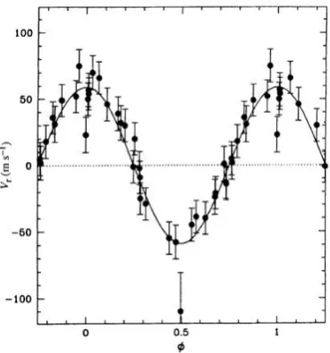
Figure 1.4: Radial velocity variations for the star 51 Peg due to the presence of a Jupiter mass planet orbiting it. From Mayor & Queloz [1995]

the star moves towards or away from an observer on Earth. Spectroscopic observa-tions of systems with exoplanets can reveal this perturbation from Doppler shifts of the spectral lines in the form of periodic sinusoidal variations in the radial velocity. This technique is by far the most successful at finding exoplanets, and is often used to confirm candidates found by other methods. Indeed, the first ever planet discov-ered orbiting a main sequence star, 51 Peg b, was found via this procedure [Mayor & Queloz, 1995]. Figure 1.4 contains the radial velocity curve of this planet, in which variations of 60ms 1 are found to take place. This is a gas giant planet on a short 4.23 d period around its host star, an unexpected discovery since planet formation close to a star is not likely to take place [e.g. Bodenheimer et al., 2000; Ida & Lin, 2004]. This marked the start of a substantial acceleration in exoplanet research and modelling of planetary systems. Current models that explain the existence of hot jupiters tend towards a migratory evolution, where the planet is formed in the outer part of the system and migrates inwards [e.g. Michael et al., 2011].

(22)

Figure 1.5: Radial velocity variations for the star HD156846 due to the presence of a Jupiter mass planet orbiting it. From Tamuz et al. [2008]

a highly eccentric exoplanet with measured parameters ofe'0.85 and!'52.23 . A simple comparison with the radial velocity signature of 51 Peg b shown in Figure 1.4, which exhibits no measurable eccentricity, shows a clear contrast in the shapes of the curves due to the disparate eccentricities of the orbits of the planets.

The semi-amplitude of the radial velocity measurements equate to Mpsini

(23)

⌫ =Ksin ✓₂_⇡_T

P ◆

or ⌫=Kcos ✓₂_⇡_T

P ◆

. (1.2)

Naturally, this technique is more sensitive to high mass planets close to their par-ent stars. However, modern spectrographs are capable of achieving a precision of 1.5ms 1 because they have no moving parts and are vacuum sealed for ultimate stability [Pepe et al., 2000]. The High Accuracy Radial Velocity Planet Searcher (HARPS) instrument [Mayor et al., 2003], used primarily on the ESO’s 3.6m tele-scope in La Silla, is an ´echelle spectrograph operating in the 378 691nm range re-sponsible for the discovery of a large number of planets, including 9 planets around M-dwarf stars showing that it is indeed possible to form planets around lower mass stars. However, stellar features, such as spots, pulsations and activity are becoming the ultimate limitation to the radial velocity method. It is now becoming necessary to obtain long baseline radial velocity measurements before the stellar activity is understood and any planetary signal becomes evident. Moreover, asteroseismology information of planet host stars is providing more accurate masses and ages, which can only be achieved through longer base line observations of both radial velocity and photometry [e.g. Borsa & Poretti, 2012; Gilliland et al., 2011].

(24)

1.2.3 Gravitational Microlensing

Microlensing events occur when the light from a distant object (source) is observed as a foreground object (lens) passes close or in front of it. The gravitational field of the lensing object bends the light path from the distant source acting as a lens, thereby focussing its light. During this process, the lens star splits the source into two images with distorted shapes that follow curved trajectories around the lens star. These 2 images have separations of the order of the Einstein radius, which is the characteristic projected angle of gravitational lensing in general [Einstein, 1936], and are typically unresolved (1mas). Nevertheless, the total area of these 2 images is larger than the area of the source, causing it to appear brighter. Figure 1.6a shows the projected view of this event, where two images of a source (S) are produced by the gravitational field of a lens star (L). The dashed line shows the Einstein ring, with Einstein radius Re. The presence of an additional body with

projected separation close to the paths of these images in the lensing system acts as an extra lensing factor for a short period [Seager, 2010b]. The first suggestion that microlensing events could be used to detect planets was done by Paczynski [1991] and surveys of the galactic bulge such as the OGLE project [Szyma´nski et al., 2000] have detected 15 of these examples2.

In the case where the lens star contains another body orbiting it with pro-jected separationa, the second lens introduces an extra lensing e↵ect, similar to a perturbation on the original lens, providing extra magnification at those times when the object is aligned with either image of the background source. The duration of this extra magnification event depends upon the mass ratio of the two elements in the binary system,q =Mp/M⇤. The larger the mass of the companion, the longer

the event, and Earth-mass planets can have typical time scales of 3-5h [Perryman, 2011]. The projected orbital separation can be scaled with the Einstein radius as

d=a/Re, which is a crucial parameter in understanding the shape of the

microlens-ing light curve. In optics, the envelope of reflected or refracted light by a curved surface is denominated ascritical lines, and the point in the source plane where this envelope originates is called thecaustic. In the case of the binary lens system, the companion to the lens star (in this case, a planet) causes a perturbation of the crit-ical lines, generating one extra large diamond-shaped caustic ifd >1 and two small triangular-shaped caustics close together on the opposite side of the lens if d < 1 [Wambsganss, 1997]. As the source moves across the lens system, it will come close to these caustics and lensing events will occurs for each. The large caustic d > 1

(25)

configuration is more sensitive to planets, since the chance of the source crossing this region is greater, and the magnification is also larger.

Figure 1.6b shows the light curve of a planetary microlensing event [Bond et al., 2004]. In a typical case the light of the source star is enhanced for a period of time as the lensing object crosses the path of the light. However, the presence of a planet is inferred from the short peaks in the early part of the light curve when the additional body causes a further magnification to occur. The large magnification implies ad >1 configuration, and indeed the best fit givesd= 1.120.

Note that the flux of the source star is increased by a factor of 8 at its maxi-mum (without considering the perturbation of the planet), and that the duration of the event spanned 60 days. Microlensing events are now often observed by several di↵erent instruments around the globe, since such occurrences can be identified in the early stages and follow-up can be triggered immediately.

The remarkable advantage of this technique is that the magnification is higher for planets outside the Einstein radius than those at close separations from their host star. Hence microlensing is more sensitive to planets in long orbits, but a confirmation of these is extremely hard, especially since microlensing events are unique and not repeatable. Nevertheless, lensing events due to Earth-like planets have typical time scales of hours, and longer for larger values of q (Jupiter-like planets), making this a prime technique for probing planets at large separations, irrespective of their mass, that are not easy to image directly. This is a region of parameter space where most other methods are not sensitive.

1.3 Transiting exoplanets

For any multiple body system there is a chance that the orbital inclination is close to 90 and that periodically the two bodies will appear to cross in front of each other. This is the case for transiting planets, which are the main focus of this thesis. If the projected disk of the planet is large enough, a significant portion of the stellar light is blocked during transit and a characteristic dip in the luminosity can be detected. This e↵ect is small, with the typical transit depths around 1% or 0.01mag for Jupiter-sized planets orbiting a Solar-like star. Naturally, planets with radii similar to the Earth exhibit shallower eclipses with depths under 1⇥10 4, but depths up to 7% can occur around M dwarfs and more for planets orbiting white dwarfs [e.g. Faedi et al., 2011].

(26)

(a) Microlensing event projected view (b) Light curve of microlensing event

Figure 1.6: Left panel: Schematic view of the projected view of a microlensing event. This is plotted in the lens’ rest frame, so the background source (S) moves behind the system, and the images I and I+ produced by the gravitational field of the lens star (L) are shown. The two images remain colinear along the line visible. The dashed line represents the Einstein ring. Modified From Paczynski [1996]. Right panel: Microlensing event light curve of OGLE 2003-BLG-235. The inset Figure shows the data for this target spanning the 2001-2003 period. From Bond et al. [2004]

of known exoplanets discovered by radial velocity observations. The first result of such e↵orts was the detection of the planetary transit of HD209458b. Henry et al. [2000] and Charbonneau et al. [2000] independently detected the characteristic dip of this event, the latter one presenting two transits spanning 2.5 hours at a depth of ⇡1.5% separated by 3.5 days, a period consistent with the radial velocity measurements taken previously. Figure 1.7 shows the published light curve with the best fit. This is a 0.714MJ planet that orbits its host star at a separation of 0.046AU [Southworth, 2009] and is one of the most important exoplanets found to date due to the high brightness of the host star and proximity to the system. It orbits a V = 7.65 magnitude star at a distance of 47pc. The close-by nature of this system is particularly useful since the distance can be measured through parallax and therefore a more precise measurement of the intrinsic brightness is possible. This, combined with the high brightness of the target and the relatively deep transit make it a perfect case for detailed studies. Thus, it is not surprising that this planet has the largest number of associated scientific publications of any known exoplanet.

(27)

Figure 1.7: Transit light curve of the first ever detected transiting exoplanet, HD209458b. It shows the relative flux of the host star as a function of time, with the best fit. From Charbonneau et al. [2000]

found to transit through photometric follow-up at predicted times based on the radial velocity curves [e.g. Kane, 2007; Kane et al., 2009]. However, the vast majority of discoveries of currently known transiting exoplanets come from dedicated wide-field surveys scanning the entire sky in search for the tale-tell signs of eclipses (see Section 1.4). Ground-based searches such as the HATNet project [Bakos et al., 2002] and the SuperWASP project [Pollacco et al., 2006] use small aperture wide-field telescopes to systematically survey the whole sky in search of transits. These instruments can detect transit depths of_⇡1%, making them sensitive to hot Jupiters on short orbits around bright stars. This explains the clear bias towards short period high-mass planets found via the transit method in Figure 1.1, which is very useful in terms of follow-up studies.

Transit light curves

(28)

(a) Schematic of the orbit of a transiting planet (b) Schematic of a planetary transit

Figure 1.8: Left panel: Schematic view of the orbit of a transiting planet. This Figure shows the illustration of the primary (transit) and secondary (occultation) eclipses with some emphasis on the visible phases of the planet. The e↵ect of the di↵erence between the day and night sides of the planet is negligible in most cases. Right panel: Schematic projected view of a planetary transit, indicating the important points of contact (tI, tII, tIII and tIV) and the impact parameter b, as

well as the transit depth . From Seager [2010b]

characterise the light curve: the periodP; the transit depth ; the transit duration

tT, defined as the di↵erence between the first (tI) and fourth (tIV) contacts; and

the time di↵erence between the second (tII) and third (tIII) contact, essentially

the duration of the flat part of the transit tF. The period of the orbit is simply

calculated from the separations of the observed eclipses. The analytic solutions for the depth and duration of the transit tT are given by

= ✓_R

p

R_⇤ ◆2

(1.3)

and

sin(tT⇡/P) =

R_⇤ a

(

[1 + (RP/R⇤)]2 [(a/R⇤) cosi]2

1 cos2_i

)1/2

. (1.4)

The duration of the middle contactstF is scaled to the total duration of the transit

according to

sin(tF⇡/P)

sin(tT⇡/P)

= 1 (RP/R⇤)]

2 _[(_a/R

⇤) cosi]2 1/2

{1 + (RP/R⇤)]2 [(a/R⇤) cosi]2}1/2

. (1.5)

(29)

radiusR_⇤ from stellar models, and therefore measurements of the planetary radius

RP, orbital separationaand system inclinationican be performed. It is important

to note that the accuracy of these is highly dependent on the prior knowledge of stellar parameters, typically using a similar approach to that of Mandel & Agol [2002]. This method relies on determining the stellar mean density from measure-ments of the orbital period,R_⇤/a and Kepler’s Third Law and using stellar models to infer the remaining parameters using evolution models that reproduce the mass-luminosity-radius-composition relations followed by real stars. A comparison of the results of this method with more accurate measurements from asteroseismology or eclipsing binaries by Brown [2010] shows that up to 4% discrepancies can arise. Therefore, care must be taken to consider the e↵ects of such model dependence.

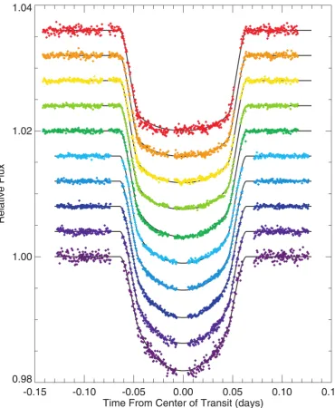
The shape of the light curve is further a↵ected by a phenomenon associated with a combination of optical depth and variations of stellar density and tempera-ture at di↵erent altitudes. This e↵ect, known aslimb darkening, causes the transit to appear shallower than when the planet crosses the edge (limb) of the stel-lar disk and deeper in the middle [Milne, 1921]. Naturally, this darkening is also wavelength dependent, larger for shorter wavelengths (higher temperatures), and was first accurately modelled by Deeg et al. [2001] for a single main sequence star other than the Sun. This e↵ect is very significant for planetary transits, however, as it is clear from Figure 1.9. This Figure shows a collection of observations of the transit of HD209458b using the Hubble Space Telescope at wavelengths ranging from 0.32µm to 0.97µm [Knutson et al., 2007]. The impact of this phenomenon is typically approximated by the fourth order Taylor series as

I(r) = 1 4 X

n=1

cn(1 µn/2) (1.6)

provided the transit observations are sufficiently precise [Claret, 2000]. In this equa-tion,µ= cos✓, where ✓ is the angle between the normal to the stellar surface and the line of sight to the observer andcn are a set of coefficients that can either be

calculated from stellar atmosphere models or directly fitted using the transit light curve. The result is a function that describes the further fractional decrease in flux as a function of what part of the stellar disk the planet is crossing in front of.

(30)

[image:30.595.135.506.137.588.2]

(31)

darkening is usually ignored.

Light curve fitting for planetary transits is often done simultaneously with radial velocity measurements, since both can provide constrains to the orbital period and, together, solve certain degeneracies. An important factor, as mentioned in Section 1.2.2, is the fact that radial velocity measurements alone provide only a lower limit to the mass of the planet, due to the MPsini degeneracy. Using the transit

light curves, the inclination of the system is uniquely determined, and therefore the mass of the planet can be calculated. Moreover, equations 1.3 to 1.5 assume a non-eccentric system, which is frequently an oversimplification. Despite the fact that a recent study by Pont et al. [2011] suggests that, for a number of systems, their non-zero eccentricities in the literature can be attributed to statistical biases and that a circular orbit is a compatible solution, planets in eccentric orbits are clearly present in the sample.

The duration of a planetary transit su↵ers from a degeneracy with the ec-centricity of the orbit. Kipping [2008] have developed a model that describes the transit light curve shape including the eccentricity [Ford et al., 2008], and the ana-lytic solution is given by

tT '

P R_⇤ ⇡ap1 e2

(✓ 1 +RP

R_⇤ ◆2

b2 )1/2_✓

rt

a ◆

, (1.7)

assumingRP ⌧R⇤ ⌧ a. In this equation b is the impact parameter andrt is the

planet-star separation at the time of mid-transit, given by

rt=

a(1 e2)

1 +ecos!. (1.8)

The impact parameter is defined simply as b_⌘acosi/R_⇤ and is used often in the fitting process to represent the optimised value of the inclination. This equation simplifies back to the expression shown in equation 1.4 fore= 0. Luckily, the shape of the radial velocity curve provides a direct measurement of this eccentricity, as well as the argument of the pericentre (see Section 1.2.2), and when combined with transit observations, a unique solution can be found.

(32)

1.4 Transiting exoplanet surveys

Modern astronomical surveys are often robotic in nature and are designed to observe whenever possible. Ground-based exoplanet surveys in general have been responsible for the majority of discoveries of known transiting planets to date. The typical principle of these surveys, since there is no a priori knowledge of which stars will contain planets in well aligned orbits for transits to be detected, is to frequently monitor the brightness of a large number of stars in search for periodic drops in flux. In the early days of the development of these surveys the predicted yield of such projects was very optimistic [Horne, 2001; Gillon et al., 2005], but as the surveys begun to operate, the stringent requirements necessary to consistently detect planetary transits became obvious.

It quickly became clear that detections of this type of planets require ded-icated telescopes and are subjected to optimizing several factors. The telescope aperture, exposure times, wavelength range and stellar distribution are among the most important, as these a↵ect the number of stars monitored of any stellar type. Larger apertures (wide-field surveys) and longer exposures generally increase the numbers of monitored stars, but increasing both these factors contributes to de-creasing spatial resolution and possible over-crowding, depending on the choice of observed fields. These problems have been approached in recent studies aimed at predicting the yield of transit surveys [e.g. Beatty & Gaudi, 2008; Heller et al., 2009], and the advantages of combining several surveys have been considered by Fleming et al. [2008]. The next Sections describe examples of such surveys. The SuperWASP project is the world leadingground-based transiting exoplanet survey, whilst the Kepler space telescope is the leading space-based project. We also de-scribe a new ground-based survey, the Next Generation Transit Survey (NGTS), which builds from the experience of the SuperWASP enterprise to search for smaller planets.

1.4.1 SuperWASP

(33)

Cremonese et al., 1997; Akerlof et al., 1999]. The consortium used commercially available hardware to limit the development work and begin observing as soon as possible. The prototype instrument for the WASP project, designated WASP0, monitored 35,000 stars in the Draco constellation for around 2 months as well as observing transits of HD209458b [Kane et al., 2004, 2005], which tested and demon-strated the principle under typical observing conditions. It used a Nikon 200mm, f2.8 telephoto lens attached to an Apogee AP10 CCD camera and operated during 2000 in La Palma and during 2001 in Kryoneri (Greece).

Science goals

The project was designed to search for bright transiting exoplanets suitable for spectroscopic and photometric follow-up studies orbiting mainly Main-Sequence stars. It is capable of achieving better than 1% photometric precision for stars in the V_⇡7 11.5 magnitude range whilst observing stars down to a limiting magnitude of V=15 [Pollacco et al., 2006]. Despite being able to survey the entire visible sky in just 40 minutes, the project was designed to observe a choice of fields per night in relatively high cadence, visiting each field at an average of 7 minutes [Smith et al., 2006] in a cyclic fashion for approximately 100-150 days each year. This strategy is sensitive to large planets in close-in orbits, which exhibit transits of approximately 1% depth every few days. It is currently the most successful ground-based transiting exoplanet survey in history, having discovered over 60 confirmed planets to date3.

Observatories and hardware

Each facility comprises of a two-roomed enclosure incorporating a roll-o↵ roof design housing a single telescope mount and the computer hardware systems to control the instrument. The telescope mount, capable of a pointing accuracy of 30 arc second rms over the whole sky and yet providing a slewing rate of 10 degrees per second, is constructed by Optical Mechanics Inc. (Iowa, USA) and contains 8 2kx2k Andor Technology (Belfast, UK) CCD cameras with 13.5µm pixels. These are back illuminated chips with QE peaking at over 90%, operating at a temperature of 50 C, through a five stage thermoelectric cooler where the dark currently has been measured to be negligible (_⇡11e/pix/h). Figure 1.10 shows a picture of the SuperWASP South facility. Canon 200mm, f1.8 telephoto lenses are used for each camera, providing a field of view of_⇡64 square degrees for all 8 cameras arranged in a 2x4 disposition [Pollacco et al., 2006].

(34)

[image:34.595.123.523.126.653.2]

(35)

[image:35.595.128.510.110.391.2]

Figure 1.11: Wavelength response of the SuperWASP instrument. The top panel shows the passband of the SuperWASP filter alongside the atmospheric and optics transmission and the CCD QE curve. The bottom panel shows the original unfiltered system alongside the Tycho 2 V filter response for comparison. From Pollacco et al. [2006]

The telescopes use a broad passband filter at the 400 - 700 nm wavelength range which, when combined with the atmospheric and optics transmission func-tions, provides an instrument response as presented in Figure 1.11. This broadband approach has the advantage of maximising the collected flux at optical wavelengths, thereby maximising the number of available targets. However, color di↵erences are likely to be an issue that requires calibration.

(36)

North facility observed 6.7 million stars and collected 12.9 billion data points [e.g. Christian et al., 2006; Lister et al., 2007] and the archive has been publicly released to the scientific community [Butters et al., 2010].

Once the data has been reduced, the process of looking for planetary transits takes place. In most surveys this is done using a modified box-least squares (BLS) algorithm such as that presented by Kov´acs et al. [2002]. This algorithm folds the light curve over a set of periods of interest and attempts to fit a rectangular shaped function to the data. This fit can then be refined using transit profile models at a later stage [Protopapas et al., 2005]. Other authors have proposed and analysed alternative search methods in order to maximise the scientific output of these surveys [Aigrain & Favata, 2002; Aigrain et al., 2004; Tingley & Sackett, 2005; Moutou et al., 2005; Collier Cameron et al., 2006; Ford et al., 2008]. This identification is complicated by the presence of a number of other astrophysical events that mimic planetary transits. Star spots on the surface of stars can produce periodic dips in the light curves, as well as eclipses from binary systems and ellipsoidal variations [Willems et al., 2006]. The selection of planetary candidates is, therefore, simply a selection of targets that then require further follow-up with larger telescopes in order to disentangle scenarios such as those mentioned.

Only the most promising candidates are chosen for follow-up. Photometric follow-up can identify any cases where aperture blending has taken place and the period dips coming from eclipsing binaries whose flux has been contaminated by another nearby star. Double-lined eclipsing binaries can be normally identified by a single spectrum and a set of radial velocity measurements are required to indeed confirm the sub-stellar nature of exoplanets.

History and discoveries

The various planets found by this survey have challenged our understand-ing of the structure and formation of such exotic bodies. Because SuperWASP is sensitive to close-in large planets it has found examples of bodies under extreme conditions of temperature, irradiation and density. Moreover, the sheer number of planets found has contributed to a rich and diverse sample of exoplanets.

(37)

the rotational spin of the star. This is also the SuperWASP planet with the longest period found to date. Due to the short baseline of coverage of each field (around 4 months) and the stringent requirements for a convincing detection of transits, the instrument is not sensitive to planets on orbital periods over 10 days and this is the highest trial period of the transit searching algorithm.

The case of WASP-12b [Hebb et al., 2009] is of particular importance. At the time of its announcement it was the exoplanet exhibiting the largest radius (1.79RJ) and shortest period, completing an orbit around the host star in just

over one day. This made it the most heavily irradiated exoplanet known to date, with a predicted surface temperature of 2516 K and triggered a series of follow-up studies to determine its atmospheric properties. The presence of an extended exosphere around the planet with absorption from Na and Mg II has been suggested by Fossati et al. [2010], where enhanced transit depths are detected in near-UV observations. Secondary eclipse observations of this planet using both space and ground-based telescopes have revealed a high brightness temperature of around 3000 K, which initially suggests a low albedo and poor redistribution of the heat around the planet [L´opez-Morales et al., 2010; Campo et al., 2010; Croll et al., 2011; Zhao et al., 2012]. However, recent observations by Crossfield et al. [2012] using the low-resolution prism on IRTF/SpeX suggest otherwise, showing that a 200-1000 K day/night e↵ective temperature contrast is possible, and that therefore an efficient heat redistribution around the planet is probable. The low density of this planet makes it a good candidate for transmission studies (see Section 1.5.4) and this example has demonstrated that ground-based telescopes are capable of achieving enough quality for such studies.

The discovery of WASP-17b [Anderson et al., 2010b] had an immediate im-pact. This is the lowest density planet known to date, with a mass of 0.49MJ

but a radius of _⇡ 2RJ and therefore a prime candidate for studies of planetary

atmospheres. Transmission spectroscopy of this planet has been performed from the ground [Wood et al., 2011], where the authors detect a depletion of sodium compared to the expected levels from a cloud-free atmosphere with solar sodium abundance. Moreover, secondary eclipse observations using the Spitzer space tele-scope at IR wavelengths have found the brightness temperature to be around 1500K and suggest a low albedo with efficient heat redistribution around the planet.

On the opposite end of the scale to WASP-17b in terms of density, the massive and extremely dense exoplanet WASP-18b (10MJ but 1.16RJ) orbits its host star

(38)

that further study of exoplanet atmospheres is crucial towards understanding these bodies. Moreover, the shortest orbital period exoplanet known to date, WASP-19b [Hebb et al., 2010], which circles the host star in 0.79 days, has challenged models of planetary orbital stability [Hellier et al., 2011] and has triggered several observations of its secondary eclipse. The thermal emission detections of this planet [Anderson et al., 2010a; Gibson et al., 2010] suggest a brightness temperature of over 2500K and a zero albedo and poor heat redistribution model just manages to explain such high levels. The authors suggest that the model used is potentially too simplistic and advise that further measurements are required to better constrain the parameters.

Other examples of particularly interesting SuperWASP planets include WASP-29b [Hellier et al., 2010]. This is currently the lowest mass planet found by this survey. With a mass of 0.24MJ, it is a Saturn-mass planet orbiting a K4 dwarf

star. This planet is given as an example of the potential of the project to push towards smaller planets (see Section 1.5.3). WASP-34b is also a sub-Jupiter mass planet that has been found to orbit a hierarchical triple system. The planet orbits the main star every 4.31 days in a slightly eccentric orbit, but a linear trend in the radial velocity curve of 55ms 1 suggests the presence of an additional body in the system, thought to be either a long period star or an extra planet [Smalley et al., 2011].

A final example of an outstanding discovery is the case of WASP-33b [Collier Cameron et al., 2010]. This planet orbits a hot, fast-rotating A5 star and is the first ever known planet to orbit a Scu host star [Herrero et al., 2011]. It is also the hottest known planet found to date, with an estimated surface temperature that exceeds 2700K. The authors find evidence of non-radial pulsations present in the radial velocity measurements distinct from the planet signal, which suggest tides created by the planet on the surface of the star. Moreover, a secondary eclipse detection of this object points towards a brightness temperature in the z-band of

⇡3600K, suggesting zero-albedo and inefficient heat redistribution from the day to the night side of the planet. However, due to the presence of stellar pulsations, the detection of the secondary eclipse required those to be modelled and removed. Since the baseline of the observation was relatively short, the remaining light curve shows large residual e↵ects of this decorrelation, and further observations are required.

1.4.2 Kepler

(39)

observations are possible. In this context, NASA’s Kepler satellite was launched into a heliocentric orbit trailing the Earth’s path [Borucki et al., 2010b; Koch et al., 2010]. The 0.95m modified Schmidt telescope houses 42 2Kx1K CCDs simultane-ously monitoring the brightness of 150,000 main sequence stars in its 105 square degree field of view. 4 fine guidance sensors provide accurate pointing and the tele-scope is deliberately defocused to 10 arcsec to improve photometric precision over the 30 second integrations taken. The mission was launched in March 2009 and the first results have been announced recently.

Science goals

The space craft is capable of achieving a 4 detection of an Earth-mass planet orbiting a 12th magnitude G2 dwarf star (Sun-like) over 6.5 hours [Borucki et al., 2010b]. The objectives of this mission are varied but are mainly oriented towards exploring the structure and diversity of extrasolar planetary systems. It achieves this by detecting planetary transits around a large sample of stars, which will help determine the frequency of terrestrial and larger planets within the habitable zones of their parent stars. This will also aid in providing an insight into the distribution of planet radii and orbital separations for exoplanets in order to understand if the particular case of the Solar System is an exception in these terms.

The high precision photometric measurements and long baseline of observa-tions will also allow the discovery of multiple planet systems which can be used as case studies of the orbital stability and frequency of such systems. Moreover, this is the first project capable of detecting the variations in reflected light from close-in highly irradiated planets as they orbit the host stars. Results of such observations will provide a direct measurement of the albedo of these planets, a critical parameter to understand the optical properties of the atmosphere of exoplanets.

(40)

Important discoveries

As of 30th August 2012, the Kepler team has announced the discovery of 77 confirmed planets4. The following examples highlight some of the most important cases in the context of exoplanet exploration.

The first new planet detected, Kepler-4b [Borucki et al., 2010a], is a Neptune-sized planet on a 3.2 day orbit around a late G0 star. The designations 1-3b are reserved for previously known planets in the Kepler field (TrES-2b [O’Donovan et al., 2006], HAT-P-7b [P´al et al., 2008] and HAT-p-11b [Bakos et al., 2010] respectively). This is a typical example of a hot-Neptune but demonstrates the photometric pre-cision of the Kepler instrument. Figure 1.12 shows the Kepler light curve for this planet. Note the depth of the transit is 1mmag, which is an order of magnitude smaller than the typical depth of a Hot-Jupiter.

The first planetary system found with multiple transiting planets was that of Kepler-9 [Holman et al., 2010]. This system contains two planets that transit the disk of the host star every 19.2 and 38.9 days for Kepler-9b and Kepler-9c respectively. These show detectable transit timing variations of 4 and 39 minutes due to each other’s presence, consistent with a 2:1 resonance motion, but once these trends are removed evidence of a third planet is presented, corresponding to a super-Earth-sized planet on a 1.6 day period orbit, later confirmed by Torres et al. [2011]. The case of the Kepler-11 has, however, revolutionised the field of exoplanets [Lissauer et al., 2011]. At the time of its announcement, this star system showed the largest number of transiting exoplanets orbiting the same star to date. 6 planets were found to transit this star, Kepler-11 b-f showing orbital periods between 10 and 47 days and Kepler-11g at ⇡ 118 days. This system is an excellent case for studies of the stability of orbits of multiplanetary systems [Migaszewski et al., 2012]. Moreover, the masses of planets in multiple systems can be measured from the timing variations caused on the others. The Kepler team have recently confirmed the discovery of another system with 6 planets orbiting it, Kepler-33 [Lissauer et al., 2012]. Using this system as a test case, the authors argue that systems showing transits of multiple planets are unlikely to be false positives, and that validation is possible without resorting to radial velocity measurements.

Kepler-10b represents the first ever rocky planet found by the Kepler instru-ment [Batalha et al., 2011]. This 4.56M and 1.42R planet orbits it’s host star in just over 45 days and represented a significant result, as it was the smallest planet ever found at the time via the transit method. The subsequent discovery of the

(41)

(42)

Figure 1.13: Kepler light curve of planet Kepler-16b. The top panel shows the unfolded detrended light curve with each of the eclipses color coded, corresponding to the cases shown in the bottom panels. The blue eclipses are those where star B eclipses star A (the larger star) and the yellow eclipses show the reciprocal event. The green eclipses correspond to the transit of the planet across star A, and the red the transits across star B. From Doyle et al. [2011].

Kepler-20 system was another milestone, containing 5 planets in total, 2 of which are smaller than Kepler-10b [Gautier et al., 2012; Fressin et al., 2012]. Kepler-20e (1.08R ) and Kepler-20f (0.87R ) represent some of the smallest planets ever found. A recent analysis of the Kepler Object of Interest (KOI) 961, also known as Kepler-42, suggest the presence of 3 planets orbiting an M dwarf star with radii smaller than the Earth, Kepler-42d being Mars-sized (0.57R ). These cases show the power of this mission and the particular advantage of intensive coverage of a single field from space.

Perhaps the most impressive result from this mission is the discovery of the first ever circumbinary planet by Doyle et al. [2011]. Kepler-16b orbits a pair of low-mass stars (Kepler-16A and Kepler-16B) over the period of 229 days. The stellar binary’s 41 day orbit is eccentric but the motions of the three bodies are confined to within 0.5 of a single plane, consistent with a disk formation scenario. The light curve for this particular system contains the transits of the planet as it travels across the disks of both stars, as well as the deep stellar eclipses, as shown in Figure 1.13. The top panel shows the detrended light curve, with the several eclipses color coded according to the corresponding cases outlined in the bottom panels.

(43)

with the multi planetary transiting systems mentioned earlier, seem to suggest a disk formation scenario is likely to be the viable solution for these cases. Indeed, these discoveries have motivated the question of whether this is indeed the case at all times [e.g. Meschiari, 2012; Paardekooper et al., 2012]. However, since Kepler is not sensitive to multi planetary systems that are non-coplanar, this question remains unanswered.

Despite the generous number of confirmed planets by this mission, perhaps the most useful and remarkable science output of the Kepler instrument has been the announced of over 2,300 planetary candidates that are yet unconfirmed. Gautier & Kepler Science Team [2010] describe several methods to reject false positives, such as careful analysis of the light curves in search of features common to eclipsing binaries, spectroscopic follow-up and multi-band photometry such as that performed by Col´on et al. [2012] in which signs of eclipsing binary behaviour can be detected.

The large number of candidates provides an opportunity to perform reliable statistics even if only a fraction of those are indeed later shown to be real planets. An example of such study is that performed by Kane et al. [2012]. Lissauer et al. [2012] argue that most of the planetary candidates are true on the basis that there are around one hundred times more candidates in multi-planetary systems then what would be expected from a random distribution of candidates. This conclusion is supported by the empirical analysis of Morton & Johnson [2011], where the authors conclude that over 90% of Kepler candidates have a probability of being a false positive of less than 10%.

Finally, the discovery of the first Earth-like planet in the habitable zone of its host star [Borucki et al., 2012b] marks the ultimate accomplishment of this mission. Kepler-22b is a 2.38R planet on a 290 day orbit around a G5 dwarf star. The radiative equilibrium temperature for a planet on this orbit is of 262K and, despite the fact that only an upper limit to the mass of this planet of 124M (with a 3 confidence) from radial velocity measurements is available, this is the closest to an Earth analogue of any exoplanet known to date.

1.4.3 The Next Generation Transit Survey

(44)

[Pollacco et al., 2006], and has recently secured full funding and authorisation to be commissioned early 2013 at ESO’s Paranal Observatory in order to benefit from one of the world’s premier sites.

NGTS has the potential to find Earth-like planets around smaller stars and, because the covered area is larger than that of Kepler [Koch, 2010] (>1500deg2), it will find transiting planets around bright stars, which are those where atmospheric follow-up studies are possible with facilities such as the Hubble Space Telescope, the Very Large Telescope (Chile) and all the planned large telescope facilities (ESO’s E-ELT, ESA’s ECHO mission and NASA’s concept FINESSE). It will achieve this by monitoring the brightness of all the visible targets within its field-of-view in search of periodic dips, which are the tell-tale signs of the existence of transiting planets. Contrary to the SuperWASP project (see section 1.4.1), which is an almost all-sky survey that samples several pointings every night, NGTS will employ astaring

strategy in which it will observe one field for as long as possible (typically around 4 months) before changing. This has the added advantage of increased precision in the time-scales of single transits (around 1-3 hours) but also, crucially, brings the potential to discover planets on longer orbits. The vast majority of transiting planets found to date orbit their host stars in typically less than 10 days (based on exoplanet.eu) mostly due to an observational bias, and only recent surveys, such as the Kepler mission, have observed a single location for a long enough time-scale to be sensitive to longer period planets [e.g. Borucki, 2012].

(45)

S´egransan et al., 2011; Pepe et al., 2004] currently mounted on ESO’s 3.6m telescope in La Silla have proven to be extremely successful in these enterprises.

The final NGTS facility will be composed of 12 fully-robotic wide-field 20cm telescopes, equipped with deep-depleted CCDs developed to the project’s specifica-tions by industrial partners (Andor Technology plc, Belfast and e2v, Chelmsford, UK). The CCD model, now available at Andor’s general range, is capable of achiev-ing high precision photometric measurements within the desired wavelength range of the instrument (600-900nm). The facility is housed in a custom designed building with a rolling roof, that will comprise of an inner chamber containing the telescopes and two side rooms for the computer servers required to control the facility and communicate with the UK. Each telescope is assembled on an individual mount, in order to achieve precise guiding and maximise the flexibility of the experiment in terms of observing strategy.

Science goals

The main objective of the survey is to search for transiting planets of Neptune-size and below around bright stars. The many recent discoveries of planetary systems harbouring Neptune-mass planets and super-Earths clearly indicate that low-mass planets around solar-type stars must be very common [Traub, 2012; Wittenmyer et al., 2011; Mordasini et al., 2009a,b]. However, very little information is available regarding the structure and composition of these planets. Moreover, planetary sys-tems such as the Kepler-11 case show that, as is the case for gas giants, there is likely to be a large diversity of earth-sized planets [Lissauer et al., 2011]. Figure 1.14 shows the optimal sensitivity range of the facility. It shows that this project is designed to explore a region of parameter space that is relatively unpopulated.

(46)

(47)

The Prototype

The ability to achieve 0.1% precision across the wifield of view is very de-manding and was demonstrated using a prototype system operated on the La Palma Observatory (Spain) during the 2009-2010 season. A smaller version of the e2v CCD (1k_⇥1k) was deployed on an 8 inch Takahashi telescope and tests were performed to determine if the desired sub-mmag precision was possible to be achieved. This puts this facility in a superb position to explore a region of parameter space that is currently relatively unpopulated, as shown in Figure 1.14. This Figure also contains information on the typical stellar types associated with each radius as well as radii of representative Solar System planets for reference. The analysis of the data taken by the prototype instrument have shown that 1mmag precision is indeed achieved, as presented in Figure 1.15. This plot displays the fractional RMS for stars in a field observed for one night with the prototype instrument as well as the expected noise based on the model to be described in Section 2.3. Transits of the Hot-Neptune GJ436b were easily recovered and a precision of 0.5 mmag is reached in one hour time scales for a star of magnitude I=10.5, which corresponds to V=12, fulfilling the science requirement.

Other tests were performed on the prototype instrument, such as the guiding capability of the telescope and flat-fielding, and results have shaped the design of the project, with the majority of telescope components already purchased. A testing system will be assembled in the Summer of 2012 by a team at the Geneva Obser-vatory for software and operations testing before the complete system is integrated on the mountain in early 2013. Other elements crucial to the project, such as data storage and mining, analysis software and knowledge of infrastructure are largely based on those developed for the SuperWASP project, making this facility science ready as soon as it is commissioned.

1.5 High-precision photometry for exoplanet research

(48)

[image:48.595.127.523.235.526.2]

(49)

are typically done in a specific wavelength range usually restricted with the use of filters, which leads naturally to spectrophotometry. This process simply involves making measurements with multiple filters to obtain a spectral profile of a given event/target.

Time series photometry is a very powerful method, not only because it can be done on many stars simultaneously (see Section 1.4) but also because of the valuable information that can be derived from it. Planetary transits (see Section 1.3) are observed through this method and hence this is the only type of photometry featuring in this thesis.

The time resolution that can be achieved is only dependent on the read-out time of the photometer used and the brightness of the target5. The use of CCDs has revolutionised the field, not only because of the relatively short read-out time but mostly because of the precision that can be obtained in terms of photon counting with respect to other options such as image sensors and photodiode cells. It does, however, have some drawbacks that have to be understood if high-precision photometry is to be achieved. Section 1.5.1 introduces these devices in detail and outlines the standard processes used to minimise these drawbacks.

1.5.1 Astronomical photometry using CCDs

Charge Coupled Devices (CCDs) have revolutionised modern astronomy. The knowledge brought by the arrival of these instruments can be paralleled with the advances due to the invention of the telescope [Howell, 2000]. In the short time since CCDs were employed in astronomy in the early 1980s, our understanding of the Universe has changed dramatically. The accuracy with which it is possible to make measurements with CCDs in contrast to photographic plates (which have a non-linear response) has brought a new era in astronomical findings. The linear re-sponse of such devices has allowed precise photometric all sky surveys to take place, as well as unprecedented accuracy and consistency in photometric measurements, leading to the discovery of exoplanets and better understanding of astronomical phenomena such as Gamma-ray Bursts, Stellar flares and Supernova explosions.

A CCD chip is generally based around a slightly p doped layer of semi-conducting silicon formed of arrays of picture elements, typically abbreviated to pixels. The major advantages of these devices are the relatively low noise, high quantum efficiency (QE) and good wavelength response in the visible range of the spectrum (typically 3,000 to 10,000 ˚A) [Martinez & Klotz, 1998] . QE is defined as

5_{If the target is very faint, it is necessary to collect photons for a long enough period of time}

(50)

Figure 1.16: Analogy of a CCD readout to a series of buckets. This image demon-strates the horizontal and vertical readout process. From Janesick & Blouke [1987]

the fraction of the incoming photons the CCD is able to convert into electrons, which is wavelength dependent. More importantly, obtaining an image from a CCD camera takes only a few seconds (readout time) and therefore testing, acquisition, inspection and analysis of the data is quick. Each pixel converts photons into electrons which can then be converted to numeric values, also known as ADUs, through analogue-to-digital converters.

The readout stage of a CCD chip follows a principle similar to that depicted in Figure 1.16. The charge in all rows is shifted to the row below via a generation of an electric potential that forces the electrons to move to the adjacent pixel. The charge in the lowest row is transferred to an additional readout row which is then horizontally shifted. The charge in each pixel is then sent onto the analog-to-digital converter where the change in voltage caused by this charge is detected by the on-chip amplifier. This process is not completely noise free, as the amplifier’s noise performance is typically a simple relation of 1/f at low sampling frequencies but displaying a white noise level at higher frequencies. This is commonly known as the readout noise. The sampling frequency is the rate at which each individual pixel is read by the CCD electronics (the readout speed). This information can then be used to reconstruct the image digitally and proceed to the calibration and analysis stages.