Original citation:
Herrera, Helios, Morelli, Massimo and Nunnari, Salvatore . (2015) Turnout across democracies. American Journal of Political Science, 60 (3). pp. 607-624.
Permanent WRAP URL:
http://wrap.warwick.ac.uk/81669
Copyright and reuse:
The Warwick Research Archive Portal (WRAP) makes this work by researchers of the University of Warwick available open access under the following conditions. Copyright © and all moral rights to the version of the paper presented here belong to the individual author(s) and/or other copyright owners. To the extent reasonable and practicable the material made available in WRAP has been checked for eligibility before being made available.
Copies of full items can be used for personal research or study, educational, or not-for profit purposes without prior permission or charge. Provided that the authors, title and full bibliographic details are credited, a hyperlink and/or URL is given for the original metadata page and the content is not changed in any way.
Publisher’s statement:
"This is the peer reviewed version of the following article: Herrera, Helios, Morelli, Massimo and Nunnari, Salvatore . (2015) Turnout across democracies. American Journal of Political Science, 60 (3). pp. 607-624. which has been published in final form at
http://dx.doi.org/10.1111/ajps.12215 This article may be used for non-commercial purposes in accordance with Wiley Terms and Conditions for Self-Archiving."
A note on versions:
The version presented here may differ from the published version or, version of record, if you wish to cite this item you are advised to consult the publisher’s version. Please see the ‘permanent WRAP URL’ above for details on accessing the published version and note that access may require a subscription.
Turnout Across Democracies
∗
Helios Herrera
Massimo Morelli
Salvatore Nunnari
HEC Montreal
Bocconi University, IGIER,
Bocconi University
and NBER
June 2, 2015
Abstract
World democracies widely differ in legislative, executive and legal institutions. Dif-ferent institutional environments induce difDif-ferent mappings from electoral outcomes to the distribution of power. We explore how these mappings affect voters’ participation to an election. We show that the effect of such institutional differences on turnout depends on the distribution of voters’ preferences. We uncover a novel contest effect: given the preferences distribution, turnout increases and then decreases when we move from a more proportional to a less proportional power sharing system; turnout is maximized for an intermediate degree of power sharing. Moreover, we generalize the competition effect, common to models of endogenous turnout: given the institutional environment, turnout increases in the ex-ante preferences evenness, and more so when the overall system has lower power sharing. These results are robust to a wide range of modeling approaches, including ethical voter models, voter mobilization models, and rational voter models.
Keywords: Voter Turnout; Voter Mobilization; Power Sharing Rules; Proportional Rep-resentation; Electoral Systems; Forms of Government.
∗We are grateful to Andr´e Blais, Gary Cox, John Huber, Navin Kartik, Suresh Naidu and Santiago
1
Introduction
Electoral participation is considered as an indication of the health of a democracy (Rose 1980, Powell 1982) and a pillar of the democratic ideal of political equality (Lijphart 1997). The
historical average turnout rate as a percentage of voting age population displays a large
vari-ance across world democracies: New Zealand, Portugal, Indonesia, Italy, and Albania have an
average turnout rate above 85%, while Senegal, Colombia, Ecuador, Ghana, and the U.S. all
have average turnout rates below 50%.1 A number of empirical papers have attempted to
ac-count for cross-national variations in turnout (Powell 1980, 1982, 1986; Crewe 1981; Jackman
1986; Jackman and Miller 1995; Blais and Carty 1990; Black 1991; Franklin 1996; Blais and
Dobrzynska 1998; Selb 2009). These studies highlight that electoral rules and party systems
are important factors affecting turnout but, by and large, do not focus on other political in-stitutions and, more importantly, neglect their interaction in determining the influence votes
have on policy outcomes.
Voters do not care about the distribution of seats per se, but rather about the overall
power to change policies conferred by those seats. Any theory of turnout should focus on the
incentives of voters and, thus, should consider the mapping from how seats are distributed
to how power is shared, not only the mapping from votes to seats. This raises an important
question: How do political institutions, that is, not only electoral rules, but also forms of
government, bicameralism, judicial review, federalism, separation of powers, committee chair assignments, and all other institutions determining the power of majority and minorities for
any given distribution of seats in a legislature, affect electoral participation in a democracy?
This paper aims to provide a set of robust theoretical predictions about how turnout varies with
the overall proportionality of the mapping from the distribution of votes to the distribution of
power, hence skipping completely the intermediate step of the distribution of seats.
A recent theoretical literature in economics and political science has compared turnout
in two extreme cases of power sharing: a winner take all benchmark where the winner of the majority of votes receives hundred percent of the power to decide on policies, and the
opposite extreme benchmark of full proportionality of the mapping from votes to power shares
(Herrera et al. 2014, Kartal, forthcoming, Faravelli and Sanchez-Pages, forthcoming). This is
unsatisfactory, as most institutional systems in use around the world are de jure or de facto
rather somewhere in between those two extremes. Not only do many countries adopt explicitly
mixed electoral systems, where two electoral rules using different formulae run alongside each
other,2 but formal and informal institutions in the legislative, executive or judicial branches
induce different mappings from electoral outcomes to the distribution of power. Examples of
such institutions include the veto power of a qualified minority in the U.S., the way margins
of victory translate into committee assignments or guarantee a more powerful mandate, the
division of powers between the legislature and the executive, federalism, the power to appoint
constitutional judges, etc.
In this paper, we develop a formal approach in order to provide rigorous foundations for the
study of the complex relationship between the proportionality of an overall institutional system
and turnout. We present a theoretical analysis of the fundamental causes of the variation in
turnout based on differences in institutions for political power sharing. Instead of exploring
all the formal and informal political institutions mentioned above, we consider all possible
determinants of the degree of power sharing in a reduced form, considering as equally important
all the different institutional components affecting the mapping from vote shares to the relative
weight of different parties in policy making (henceforth power shares). We use the “contest success function”3 and introduce a power sharing parameter, γ, that allows us to embed a wide array of institutional systems or power sharing regimes, ranging from a fully proportional
power sharing system (γ = 1) to a system with zero power sharing (γ = ∞). This modeling
innovation allows us to span continuously across all institutional systems and to analyze them.
We study the role of these institutions on electoral participation by characterizing how the
vote-shares-to-power-shares mapping affects voters’ incentives to vote and parties’ campaign
efforts. We try to develop a theory that is as robust and general as possible. First, we take into
account the distribution of political preferences in the population, a contextual factor that has
proven to be crucial in models of endogenous turnout (see, for example, Herrera et al. 2014 and
Kartal, forthcoming). Second, we allow for multiple alternative behavioral assumptions about the turnout mechanics, rather than limiting our analysis to one single approach.
We show that the effect of the institutional differences on turnout depends on the distribution
of voters’ preferences for the competing parties, or the ex-ante preference “evenness” of the
election in a non obvious way.4 In particular, we uncover a novel contest effect: given any
asymmetric distribution of preferences, as we move gradually from a relatively even power
sharing system to one that gives more policymaking power to the majority party, turnout
increases first and then decreases. Therefore, turnout is highest for intermediate levels of the
overall institutional mapping from votes to power. The turnout maximizing degree of power sharing depends on the distribution of preferences, but it is always intermediate for any
ex-3See Tullock 1980. This function is extensively used in several economic contexts, especially in the contest
literature (see among many others Skaperdas 2006) typically as a mapping from efforts or resources to the chance of victory.
4Cox (1999), as summary of the analysis of the elite mobilization section, says that “...the argument following
ante uneven election. The intuition is as follows. As we move a away from an even power
sharing system, the institutional system becomes more and more similar to a system where
power is concentrated in the hands of the party that obtains a plurality of the votes. Hence,
turnout drops for any lopsided preference distribution because the underdog side has no chance
of obtaining the plurality of the votes which is all that matters in this case. A system with
even power sharing will typically display moderate turnout for all preference distributions, as the incentives to turnout remain even in a very lopsided election: there is always a possible
power gain for turning out more. Finally and crucially, for intermediate systems, i.e. between
full power sharing and no power sharing, turnout is the highest. To understand the intuition
for this result, imagine that the preference split is 40-60 and think which institutional system
would grant the largest turnout in this case. Intuitively, such a system would be one that grants
significant power gains around an election outcome close to 40-60. Namely, an intermediate
system whose vote-shares-to-power-shares mapping is very steep around a qualified minority of
40%, so that the marginal gain from extra votes can make a significant difference in the powers
granted de jure or de facto.
In addition to this, we generalize to all institutional environments the competition effect, already well-documented in several models of endogenous turnout: given the institutional
en-vironment, turnout increases in the ex-ante preference evenness of the election and peaks when
the population is perfectly evenly split between the two parties.5 Even though such a
com-petition effect is common to all institutional systems, the sensitivity of turnout to the level
of competitiveness is higher the lower is the extent power sharing, at least when excluding
situations with especially large expected margins of victory.
We derive our results for the ethical voter model and then show that these results are
preserved in other costly voting models. These models are the voter mobilization model, which
we fully characterize, and the rational voter model, for which we provide numerical simulations
supporting the qualitative results of the previous two models. Unlike the rational voter model,
the ethical voter model, for which we conduct the core of our analysis, assumes that voters on
the two sides overcome the free-rider problem so that each side turns out at the optimal level.
This guarantees that turnout remains large in a large election, a desirable property. On the
technical side, the decreasing generalized reversed hazard rate (DGRHR) property of the cost function, a regularity condition on probability distributions, turns out to be the key sufficient
condition to obtain all the results in all group models. The equilibria from all models feature
another well documented property (see, among others, Castanheira 2003), the underdog effect. We show that, in all the models we present and for all institutional systems, the underdog effect
isnon-full, which means that the side which enjoys the majority of ex-ante support also obtains
5Several experimental works have confirmed this theoretical prediction (see Levine and Palfrey 2007, Kartal
the majority of the votes in equilibrium for all power sharing systems. This property drives all
comparative statics results we obtain, namely, the competition effect and, most importantly,
the contest effect described above.
1.1
Related Literature
Our modeling strategy is related to a body of literature that studies voters’ turnout in large
elections. Our main model is the ethical voting model (Coate and Conlin 2004, Feddersen
and Sandroni 2006). We also show the same results hold for mobilization models (Morton
1987, 1991; Cox and Munger 1989, Uhlaner 1989, Shachar and Nalebuff 1999). Razin (2000)
studies the effect of vote shares on policy platforms. He shows that vote shares communicate
information to the candidates, who consequently have an incentive to moderate their policy
when their margin of victory shrinks. Castanheira (2003) is, to our knowledge, the first paper to
consider the effect of “mandates” on turnout in large elections. Its focus is not on comparing the
size of mandates per se, but on showing that mandates have in general the effect of dramatically increasing turnout relative to political systems without a mandate effect.
A recent strand of literature—including, among others, Herrera et al. (2014) and Kartal
(forthcoming, 2014)—studies strategic voting in a rational voter framework and analyzes how
turnout varies in two extreme electoral systems (fully proportional power sharing and no power
sharing) for all levels of preference splits. These papers cannot say much about intermediate
electoral systems or, more importantly, about the overall level of power sharing of an
insti-tutional system. Kartal (forthcoming) focuses more on comparative welfare results than on
comparing turnouts. As far as turnout is concerned, Kartal (see also Herrera et al. 2014) shows that full underdog compensation, and hence a close high-turnout election, can occur
when the distribution of voting costs is degenerate (see also Goeree and Grosser 2007, Taylor
and Yildirim 2010), or is bounded below by a strictly positive minimum voting cost (see also
Krasa and Polborn 2009), but not otherwise. Faravelli and Sanchez-Pages (2014) is the first
paper comparing turnout and welfare across a wider range of power sharing rules, in the same
spirit as we do here. They obtain results in a neighborhood of elections with preferences which
ex-ante perfectly even or perfectly biased, the only tractable cases in a rational voter model.
Ours is the first paper that studies a continuum of institutional systems for a general
distri-bution of preferences in the population. Faravelli, Man and Walsch (2014) study the effect of mandate together with “paternalism”. They show, under very general conditions, that the
combination of these two factors guarantees positive turnout even in a large elections and in
a rational voter framework. In addition, they provide evidence of a mandate effect from U.S.
Finally, the paper speaks to the empirical literature which studies cross-national variations
in turnout (Powell 1980, 1982, 1986; Crewe 1981; Jackman 1986; Jackman and Miller 1995;
Blais and Carty 1990; Black 1991; Franklin 1996; Blais and Dobrzynska 1998; Selb 2009). The
theoretical results we obtain from all models, from instrumental voting to mobilization models,
depend on a key variable, namely, the expected winning margin or the closeness of the election.
While there is some empirical evidence about the relationship between ex ante closeness and turnout (Blais 2000, Cox and Munger 1989, Selb 2009), the interaction effect of the expected
closeness and the degree of power sharing of the institutional system has not been studied in
the way we propose, that is, taking into account the important mapping from the distribution
of seats to the distribution of power. The paper is theoretical but, in the Appendix, we provide
indications and examples about how future empirical research could properly take into account
the message and methodological points of this paper. In particular, if what matters for voters’
participation is the overall mapping from votes to power (not the intermediate mapping from
votes to seats), a theoretical prediction on how turnout depends on the proportionality of the
whole political system can be tested using the proportionality indices for the electoral rules only across countries with similar mappings from seats to power, for example with similar division
of power between the legislature and the executive.
The article is organized as follows. Section 2 presents the general model setup. Section 3
contains the analysis of group voting models—that is, the ethical voter model (Section 3.1) and
the mobilization voter model (Section 3.3)— and compares turnout across different institutional
environments and preferences distribution. Section 4 shows that similar results hold if we
consider, instead, a rational voter framework. Section 5 offers some concluding remarks and describes potential paths of future research.
2
General Setup
We introduce here a setup common to all models we consider. Consider two parties, A and B,
competing for power.6 Citizens have strict political preferences for one or the other. We denote by q ∈ (0,1) the preference split, that is, the chance that any citizen is assigned (by Nature)
a preference for party A (thus, 1−q is the expected fraction of citizens that prefer party B).
Beside partisan preferences, the second dimension along which citizens differ from one another
is their cost of voting: each citizen’s cost of voting, c, is drawn from a distribution with twice
differentiable cumulative distribution function F (c) over the support c ∈ [0, c], with c > 0.
6We assume two parties with fixed platforms. It would be interesting to study voters’ turnout decisions when
The cost of voting and the partisan preferences are two independent dimensions that determine
the type of a voter.
For any vote shareV obtained by partyA, an institutional systemγ determines the mapping
to the respective power shares PγA(V) ∈ [0,1] and PγB(V) = 1 −PγA(V). For normalization purposes, we let the utility from “full power to party i” equal 1 for type i citizens and 0 for
the remaining citizens.7. Hence the power shares are the reduced form “benefit” components of
parties’ (respectively, voters’) utility functions that will determine the incentives to campaign
(respectively, vote) in a given institutional system γ. In a γ−system, payoffs as a function of
the vote share are represented by a standard “contest success function”8, whereγ ranges from
1 to ∞:
PγA(V) = V
γ
Vγ+ (1−V)γ , P B γ (V) =
(1−V)γ
Vγ+ (1−V)γ (1)
This representation can accommodate a wide range of intermediate power sharing rules
between pure proportional power sharing systems (P) and systems entirely without power
sharing (M), using a single parameter in the payoff function. The two extreme cases correspond
to γ = 1 (P) and γ = ∞ (M), and for instance the intermediate case γ = 3 represents the
so-called “cube law”.9
As we discussed in the Introduction, intermediate systems which are a mixture of
pro-portional power sharing and no power sharing systems are very common and have plenty of
institutional details we do not model.10 Intuitively, we just want to capture the fact that the
larger γ is the lower the extent of power sharing in the system.
Even in a winner-take-all electoral system like the U.S. Presidential race, a large winning
margin carries with it added benefits to the winner due to a “mandate” effect, and larger
winning margins for the President can carry over to a larger majority in one or both houses of Congress, via “coattails” effect.11 Also, the fact that the legislative branch in a M system has
leverage over the executive branch and the presidency will tend to smooth out the
winner-take-7This normalization will allow us to match party utility and voters’ utilities in a simple way under all the
models that will be considered.
8See, for instance, Hirshleifer (1989). When nobody votes (α=β = 0) assume equal shares (V = 1/2). 9There are other ways to introduce a power sharing level parameter. Faravelli and Sanchez-Pages (2014)
model it as a linear combination of the payoffs in two systems, P and M. For a recent paper linking electoral rule disproportionality to platform polarization see Matakos, Troumpounis and Xefteris (2014).
10For example, in Germany, voters express two preferences, one for a candidate and one for a party: 299
members of parliament’s lower house are directly elected in single member districts; another 299 members are elected from candidate lists until each party’s seat share matches the proportion of party votes that it won.
11For an empirical analysis of such effects, see Ferejohn and Calvert (1984) and Calvert and Ferejohn (1983).
all discontinuous payoff function in the direction of a more proportional power sharing scheme.
Similarly, an increase in vote shares might have a disproportional impact on payoffs also in
electoral systems with proportional representation. For example, in parliamentary systems
that require the formation of a coalition government, a party that is fortunate to win a clear
majority of seats outright has much less incentive (or in some cases none at all) to compromise
with other parties in order to govern effectively.
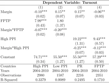
Figure 1 illustrates the power share payoff PA
γ as a function of the vote share V for three
power sharing parameters γ, namely: γ = 1 (i.e. the P system, dashed line), γ = 5 (i.e. an
intermediate power sharing system, continuous line), andγ → ∞(i.e. a pure M system, dotted
[image:9.595.143.453.314.507.2]line).
Figure 1: Power sharing function for different values of γ.
Citizens choose whether to vote for party A, party B, or abstain. If a share α of A types
vote for A and a share β of B types vote for B, the expected turnout for party A and B and
total turnout are, respectively:
TA:=qα, TB := (1−q)β, T :=TA+TB
while the expected vote shares for party A and B are respectively:
V = qα
T , 1−V =
(1−q)β T
ratio R as:
Q:= q
1−q, R :=
TA TB
We look for symmetric equilibria. These equilibria can be characterized by a voting cost threshold for each side (cα, cβ) below which supporters turn out and above which they abstain,
hence the share of A (B) supporters that turn out can be expressed byα=F(cα) (β =F(cβ)).
Henceforth, we denote as f(c) = F0(c) the probability density function of the cumulative cost
distribution functionF (c),and we callGits inverse, namelyG(α) := F−1(α) =c
α. Moreover,
we denote partial derivatives of any function Z with respect to q or γ (our main comparative
statics parameters) with the compact notation: Zq := ∂Z∂q.
3
Group Voting Models
The basic idea behind these models is that the positive externality of voting among supporters
of the same party is internalized, leading to higher turnout. The rationale behind the solution
to this collective action problem may differ across group voting models, but the end result is
that, contrary to the instrumental voting model (discussed in Section 4 below), the share of
voters turning out is high regardless of the size of the population. In group voter models, the
two sides compete in an election by turning out their supporters, which have a voting cost to turn out. The population is a continuum of measure one, divided into q A supporters and
(1−q) B supporters. In a γ−power sharing system, the marginal group benefits to the two
sides, with respect to (cα, cβ), can be derived from (1) and are, respectively:
dPA γ dcα = dP A γ dV
(1−q)β T2
qf(cα),
dPB γ dcβ
=−dP
A γ dV qα T2
(1−q)f(cβ) (2)
where:
dPA γ
dV =−
dPB γ
dV =
γ V (1−V)
V 1−V
γ
1 + 1−VVγ2
3.1
Ethical Voter Model
Our main approach to study turnout in elections, which is grounded in group-oriented behavior,
is the ethical voter model (Coate and Conlin 2004, Feddersen and Sandroni 2006). This model
assumes that citizens are “rule utilitarian” which means that they overcome the free-riding
problem and manage to act as one cohesive group. Since the ethical voter model assumes that
citizens follow the voting rule that, if followed by everyone else on their side, would maximize
the benefitPj
γ of their side from the outcome of the election minus the aggregate costCincurred
by their side. As a consequence, this model involves an equilibrium between two party-planners,
or representative agents, on each side, A and B. In the solution, each planner looks at the total
electoral benefit net of the total cost of voting incurred by his supporters, taking the other
planner’s turnout strategy as given.12 The cost of turning out the voters for the social planner on side A is the total cost suffered by all the citizens on side A that vote, namely,
C(cα) :=q
Z cα
0
cf (c)dc
Each side’s optimal voting rule specifies a critical cost level below which an individual should
vote. The citizens with cost below the planner-chosen cost threshold, cα, vote because ethical
voter models assume citizens get an exogenous benefit D(larger than their private voting cost
c≤cα) for “doing their part” in following the optimal rule established by the planner.
Defining thegeneralized reversed hazard rate as cf(c)F(c), we introduce the following definition: a distribution satisfies the decreasing generalized reversed hazard rate (DGRHR) property if and only if cf(c)F(c) is decreasing. We call it DGRHR by analogy with the known increasing generalized
failure rate (IGFR, see, for instance, Lariviere 2006), which refers to the function 1cf−F.13 If the
cost distribution satisfies the DGRHR property, we have the following result for allq∈[0,1/2].
Proposition 1 The equilibrium exists and it is unique and has the following properties:
(1) Partial Underdog Compensation: for q < 1/2, we have α > β, qα < (1−q)β, namely, underdog supporters turn out at a higher rate than leader supporters, R <1.
(2) Competition Effect: given an institutional system γ, turnout, T, and turnout ratio, R, increase in the evenness of the preference split, q.
(3) Contest Effect: given the preference split, q, turnout increases and then decreases with the unevenness of the power sharing γ; it achieves its maximum for intermediate γ.
(4) As γ goes to infinity (no power sharing), turnout goes to one when the election is ex-ante even, q= 1/2, and goes to zero otherwise.
Proof. See Appendix.
12We assume “collectivism”, so the planner on each side, A and B, only looks at the total cost of voting of
the voters on his side. The results would not change if we assumed “altruism” as in Feddersen and Sandroni (2006): each planner takes into account the cost of voting of all citizens that vote regardless of their side.
13The DGRHR is also a key regularity condition in strategic models of turnout such as Faravelli, Man and
The solution for the ethical voter model for a general γ is not straightforward to derive,
because the underdog compensation is strictly partial (rather than zero), so α 6= β, and the
two equations of the system of FOCs do not decouple. It is convenient for the analysis to
rewrite the two FOCs compactly as:
W =qαG(α) = (1−q)βG(β)
where:
W :=γ R
γ
[1 +Rγ]2
The DGRHR property turns out to be key for several reasons, not only to guarantee ex-istence, but also for the competition effect and for the contest effect. It is easy to show non
existence if DGRHR is violated, at least in certain parameter ranges. Even when existence is
granted, a violation of DGRHR can cause the competition effect to fail, that is, higher
equi-librium turnout in more lopsided elections, as we show later in an example. The DGRHR
property guarantees some regularity in the cost distribution function, so that, for instance, if
the ratio of the proportion of voters turning out from each side—α/β—increases as parameters
change, then also the cost threshold ratio—cα/cβ—increases. The latter implies, among other
things, that there is monotonicity between the relative support ex-ante and the relative
sup-port ex-post: if q, the relative ex-ante support for A, increases, then the relative turnout for A,
R =TA/TB,does too in equilibrium. For instance if 1 out of 4 citizens prefer A and 1 out of 3
voters actually voted for A (see the partial underdog effect described below), then it cannot be
that increasing the former reduces the latter, under DGRHR. We now discuss the properties
we derived in order.
(1) What seems to be a common feature across several costly voting models is the underdog
effect (see Castanheira 2003 and Levine and Palfrey 2007, among others). Namely, voting
models have the general property that the supporters for the underdog side have higher incentive to turn out than leader’s supporters. Hence, in equilibrium they vote disproportionally more
than the leader’s supporters. We call this feature “compensation” as it reduces the leader’s
initial advantage. Moreover, we call this compensation “partial” when the larger turnout of
the underdog supporters is not enough to overturn the leader’s initial advantage in preferences.
In rational voter models, partial compensation seems to be a general feature when voting costs
are heterogenous (see also Herrera et al. 2014 and Kartal Forthcoming), the reason being that
while the underdog side has higher benefits from turning out, it also bears higher costs, as it
needs to turn out more supporters, and hence will only find more supporters with higher costs.
In the ethical model analyzed here, though, the compensation effect comes from the cost side
fact identical for the two competing sides. First, because it is a zero sum game so there is a
symmetry between the incentives of one side and the incentives of the other. Second, because
the left and right derivatives are identical in a continuous model. This means that, from any
starting turnout profile, increasing marginally the turnout of one side increases the benefit to
that side as much as increasing marginally turnout for the opposite side increases the benefit to
the opposite side. Hence, the difference lies on the costs sides alone, namely, for any given cost threshold cα the underdog party has lower additional cost to turn out those additional voters.
In other words, the marginal cost is
qcαf(cα)
and it is lower for the underdog (q < 1/2). This compensation, however, is partial so the
ex-ante leader remains the ex-post leader, albeit by a lower margin. This happens because of
the termcα in the marginal cost, which means that it costs more to turn out additional agents.
This is the same logic described above for the rational voter model.
(2) We show that the competition effect is general for the ethical voter model regardless of the electoral or institutional system: the closer the ex-ante preference split, the larger the
turnout. While the competition effect seems like a very intuitive property, it is in fact not
generally true in rational voter models even with a system without power sharing.
(3) We believe the contest effect is novel: previous work has not compared turnout across
different institutional systems for all preference splits q (for extreme values of q,see Faravelli
and Sanchez-Pages 2014). The intuition is as follows: take any value of the preference split, say
for instance a 40-60 preference split (q = 40%). When γ is large the system becomes similar to a system without power sharing. Hence, turnout should be low because, despite the underdog
compensation, the underdog side has a very small chance of winning. When γ is low, the
system becomes similar to a proportional power sharing system with moderate turnout for all
preference splits. For intermediate γ, the marginal gain from extra votes can make the most
difference and this is where turnout is highest. For instance, an intermediate γ could model in
reduced form an electoral system (and possibly several other institutional details) where extra
votes for the underdog around a 40-60 outcome could mean leadership in more committees
and/or obtaining veto or filibuster powers for some decisions. Having partial (rather than full)
underdog effect is crucial for the contest effect: an election that is not a toss up ex-ante needs to remain such ex-post. If, in equilibrium, we had a 50-50 electoral outcome, then turnout
would always be increasing in γ. This is because the slope of the power function is steepest
around a 50-50 outcome in all institutional systems (for all γ >1).
(4) Lastly, in a system with no power sharing turnout is high and positive only in a very
out significantly in such an election.
3.1.1 Examples
We provide first a simple example which satisfies DGRHR. Second, to show that DGRHR is a
tight condition we provide an example that violates it and violates the competition effect.
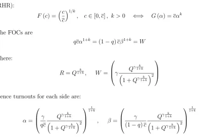
Closed Form Example Assume the cdf comes from the family (which satisfies weakly
DGRHR):
F (c) = c
c
1/k
, c∈[0, c], k >0 ⇐⇒ G(α) =cαk
The FOCs are
qcα1+k = (1−q)cβ1+k =W
where:
R =Q1+kk, W =
γ
Qγ1+kk
1 +Qγ1+kk
2
Hence turnouts for each side are:
α= γ qc
Qγ1+kk
1 +Qγ1+kk
2 1 1+k
, β =
γ
(1−q)c
Qγ1+kk
1 +Qγ1+kk
[image:14.595.80.475.235.511.2]2 1 1+k
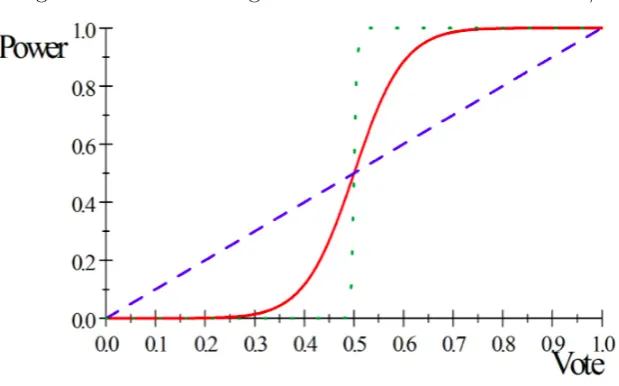
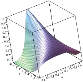
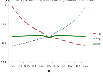
Figure 2 shows T as a function of both q and γ for the uniform distribution case (k = 1)
with c= 5.
This picture summarizes the main insights. For any electoral/institutional system γ, the competition effect is apparent: turnout increases the closer the ex-ante preference split becomes.
Fixing the preference split q, turnout is non-monotonic in the electoral/institutional system γ,
first increasing and then decreasing. For anyq <1/2, the turnout maximizingbγ is increasing in
the competitionq: the closer the election, the more uneven the power sharing in the institutional
system has to be in order to achieve its highest turnout. In other words, if ex-ante preference
splits are uneven, then more proportional power sharing systems maximize turnout; on the other
hand, if ex ante preference splits are even, systems with less power sharing achieve the highest
turnout. In sum, the electoral/institutional system that delivers the highest turnout crucially
Figure 2: T as a function of γ and q, ethical voter model.
together electoral turnout results over time in each country, never controlling for the value of
q in each election.14
Counterexample In general, from the FOCs we obtain turnout
T =γ(G(α)G(β))γ−1 G(α) +G(β) ((G(α))γ+ (G(β))γ)2
For γ = 1 we have:
T = 1
G(α) +G(β)
The cdf family
F (c) = 1−(1−c)1/m ⇐⇒ G(α) = 1−(1−α)m
c ∈ [0,1], m >0
violates the DGRHR property, as the GRHR of the inverse G(α) (see Lemma 1 in Appendix
A) is decreasing:
h(α) = mα(1−α)
m−1
1−(1−αα)m
Take for instance m= 2. For γ = 1 the FOCs are:
qα2(2−α) = (1−q)β2(2−β) =W
where:
R= β(2−β)
α(2−α), W =
α(2−α)β(2−β)
(α(2−α) +β(2−β))2
and turnout is:
T = 1
α(2−α) +β(2−β)
Figure 3 shows a violation of the competition effect. Namely, despite the presence of the
[image:16.595.118.478.409.673.2]underdog effect, total turnout is not always increasing for q∈[0,1/2].
3.2
Mobilization Model
The main message of this paper is to document the robustness of our comparative statics
results of turnout across several well known turnout models. Morton (1987, 1991), Cox and
Munger (1989), Shachar and Nalebuff (1999) and others have proposed models based on group
mobilization, where parties can mobilize and coordinate citizens to go vote. In major elections,
candidates and parties engage in hugely expensive get-out-the-vote drives. Empirical evidence
suggests that these drives are effective (Bochel and Denver 1971, Gerber and Green 2000).
There is also evidence that mobilization efforts can explain turnout variation across elections
and across electoral systems (Patterson and Caldeira 1983, Gray and Caul 2000). We adopt here a group mobilization model a la Shachar and Nalebuff (1999) where parties’ campaign
efforts and spending are able to mobilize and coordinate citizens to go vote. In this model,
each group can “purchase” turnout of its party members by engaging in costly get-out-the-vote
efforts. Thus, parties trade off mobilization costs for higher expected vote shares, taking as
given the mobilization choice of the other party.
A mobilization model assumes that more campaign spending by a party brings more votes
for the party according to an exogenous technology. We consider a very simple version of
group mobilization. We assume that the cost a party incurs in order to bring to the polls, i.e. mobilize, all its supporters with voting cost below c is l(c), where c ∈ [0, c] and l is an
increasing, convex and twice differentiable function. We also assume that it is infinitely costly
for a party to turn out all its supporters: l(c) = ∞. In addition to twice differentiability, we
assume the distribution of citizens’ voting costs F (c) satisfies a (weakly) decreasing reversed
hazard rate (DRHR, or log-concavity ofF) property.15
Under the above conditions, we have the following result, without loss of generality, for all
q∈[0,1/2].
Proposition 2 In the mobilization model, an equilibrium exists, it is unique and it has the following properties:
(1) Zero Underdog Compensation: regardless of the preference split, both sides turn out the same proportion of supporters, α = β; hence, R = Q and turnout equals this proportion,
T =α =β.
(2) Competition Effect: given an institutional system γ, turnout increases in the evenness of the preference split, q <1/2, and peaks for an ex-ante even election, q= 1/2.
(3) Contest Effect: given a preference split q, turnout increases and then decreases as the
15Note that the DRHR (also known as log-concavity of F) is weaker than the DGRHR used in the ethical
extent of power sharing drops, that is as γ increases; it achieves its maximum for intermediate power sharing systems.
(4) As the system becomes a system with no power sharing, γ goes to infinity, turnout goes to one when the preference split is even, q= 1/2, and goes to zero otherwise.
Proof. See Appendix.
The weak DRHR property of the cost distribution roughly means that the relative variation
in the number of agent-types does not increase as we span the support of the distribution.
In other words, as we increase the cost we do not suddenly find many more agents with a
given cost. This guarantees monotonicity and it is essential for a unique interior solution: the
cost-benefit ratio of turning agents with marginally higher costs is increasing.
The results for this model and their intuition are very similar to the ethical voter model,
with one caveat. The zero underdog compensation obtained in the mobilization model means
that, regardless of the electoral system and of the preference split, either side turns out the
same proportion of its supporters. The zero underdog compensation is due to the non-rival
structure of the campaign spending costs in mobilization models (see, e.g., Morton 1987, 1991,
or Schachar and Nalebuff 1999). Namely, it costs the same for either side to mobilize all their
supporters below a given voting cost threshold. In particular, it does not cost less to turn
out the same share of supporters of the smaller group than of the larger group. This is, for example, the case if one thinks of campaigning as advertising through media, which is in its
nature non-rival, but not for other forms of campaigning such as door to door persuasion, which
are clearly rival. If the latter were the case, then compensation would be partial and the results
would be similar to the ethical voter model.
3.2.1 Example: Uniform Distribution
Assume that voting costs are uniformly distributed on the unit interval, i.e., F (c) =c∈[0,1],
which satisfies DRHR, and that the cost of mobilizing voters is
l(c) = c 1−c,
which is convex on [0,1]. Then, the FOC becomes:
M B :=γ Q
γ
[1 +Qγ]2
=
l0(c)
f(c)/F (c) =
c
(1−c)2
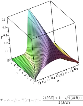
Figure 4: T as a function of γ and q, mobilization model.
T =α=β =F (c∗) = c∗ = 2 (M B) + 1− p
4 (M B) + 1 2 (M B)
Figure 4 shows T as a function of both q and γ. The similarity with Figure 2 is apparent.
Also, for any electoral/institutional system γ the competition effect is clear, as well as the non-monotonic contest effect for any preference split q.
4
Rational Voter Model
Another workhorse model for studying turnout in elections is the rational voter model (Palfrey and Rosenthal 1985). Some scholars consider the rational voter model non-satisfactory, as it
predicts very low levels of turnout in large electorates. Far from contributing to this debate,
our goal here is rather to show that, regardless of the turnout levels predicted, the comparative
statics we obtain in the rational voter model across institutional systems and across preference
splits is consistent with what we obtained in the, high turnout yielding, group models of turnout
we discussed above.
character-ized by two cutoff levels, with α=F(cα) and β=F(cβ) which solve:
M BA=G(α), M BB =G(β)
whereM BAandM BBare the marginal benefits from voting for an individual of, respectively,
group A and group B. Given expected turnout rates in the two parties, α and β,the expected
marginal benefit of voting for a party A and party B citizen are equal to, respectively:
N
X
b=0 N−b
X
a=0
[V (a+ 1, b)−V (a, b)] N!
a!b! (N −a−b)!T
a AT
b
B(1−TA−TB)N−a−b (3)
N
X
b=0 N−b
X
a=0
[V (b+ 1, a)−V (b, a)] N!
a!b! (N −a−b)!T
a AT
b
B(1−TA−TB)N−a−b (4)
where:
V (a, b) := a
γ
aγ+bγ
In equations (3) and (4), the first term in brackets in the summation is the increase in
power share as a consequence of an increase in vote shares. The remaining terms represent the
probability of the vote share being equal to a+ba without your vote, given turnout rates α and
β.16 For this model, we can offer analytical proofs for two results, existence of an equilibrium and the presence of a partial underdog effect. To show that the comparative statics discussed
for the previous models hold also under these alternative modeling assumptions, we recur to
numerical computations.
Existence. Fix N, γ and q. The pair of equilibrium conditions can be written in terms of
cost thresholds as:
M BA(cA, cB) =cA, M BB(cA, cB) =cB
Because c >1/2, M BAand M BB are continuous functions ofcA, cB from [0, c]2 into itself, and
[0, c]2 is a compact convex subset of R2.17 Therefore, by Brouwer’s theorem there exists a fixed
point (c∗A,c∗B), which satisfies both equations and is an equilibrium.
Underdog Effects. This proof is contained in Kartal (Forthcoming) and Herrera et al.
(2014). As pointed out there, in general, the partial underdog effect holds whenever a symmetric
16By convention, we denote j
j+k =.5 if j=k= 0.
17The assumptionc >1/2 guarantees that the range of these functions is contained in [0, c]2. Existence also
holds more generally for anyc >0, with only minor changes in the proof to account for the possibility thatc
power sharing functionV (a, b) (as, for instance, the purely proportional one withγ = 1 in our
model: V = a+ba ) has the property that an additional vote for the underdog has a higher
marginal impact for the underdog than an additional vote for the leader has for the leader. In
other words, the proof just hinges on following two properties of W(a, b):
W(a, b) =−W(b, a), and W(a, b)>0 if a < b
where
W (a, b) := (V (a+ 1, b)−V (a, b))−(V (b+ 1, a)−V (b, a))
While closed form analytical expressions of the equilibria do not exist, they are easily com-puted numerically. Figure 5 below shows the equilibrium overall turnout as a function of the
institutional environment, γ, and the ex-ante preference split, q, for N = 30, c∼ U[0,1], and
a benefit from winning the election of 10. This figure is qualitatively similar to the ones we
presented for the mobilization and the ethical voter models. Table 1 shows the overall turnout
as a function of γ and q for the same parameters. From these numerical computations, we can
[image:21.595.151.419.460.748.2]conclude that comparative statics similar to the one discussed for the other two models hold.
Table 1: T as a function of γ and q, rational voter model with N = 30 and c∼U[0,1].
γ
q 1 2 3 4 5 6 7 8 9 10
0.07 0.311 0.262 0.218 0.199 0.189 0.184 0.181 0.179 0.178 0.178
0.10 0.333 0.318 0.269 0.241 0.223 0.219 0.214 0.211 0.209 0.208
0.13 0.351 0.364 0.318 0.285 0.266 0.255 0.249 0.244 0.241 0.239
0.17 0.365 0.404 0.367 0.331 0.308 0.294 0.285 0.279 0.275 0.272
0.20 0.376 0.437 0.415 0.379 0.352 0.336 0.324 0.316 0.311 0.307
0.23 0.385 0.466 0.462 0.429 0.401 0.381 0.367 0.358 0.351 0.346
0.27 0.393 0.490 0.501 0.482 0.453 0.431 0.415 0.403 0.395 0.389
0.30 0.399 0.510 0.546 0.536 0.511 0.487 0.469 0.455 0.445 0.437
0.33 0.404 0.527 0.583 0.591 0.573 0.550 0.529 0.514 0.502 0.492
0.37 0.408 0.541 0.615 0.644 0.640 0.621 0.600 0.582 0.567 0.556
0.40 0.411 0.551 0.641 0.694 0.711 0.702 0.682 0.662 0.645 0.631
0.43 0.414 0.558 0.660 0.736 0.783 0.795 0.781 0.759 0.738 0.720
0.47 0.415 0.563 0.672 0.765 0.847 0.905 0.906 0.878 0.849 0.823
First, given γ, turnout increases in the size of the underdog group and peaks when the
preference split is even. This is an analogue of the competition effect we discussed in the
previous two models. Second, turnout increases and then decreases as we approach a system
with no power sharing (that is, asγgrows). In the large majority case, i.e., an uneven preference split (for example, NA= 4 whenN = 30), turnout is maximized for γ = 1 and decreases as we
increaseγ. When preferences are closer (for example,NA= 10 whenN = 30), turnout initially
increases as we increase γ. As the power sharing of the system becomes less proportional,
winning the election becomes paramount so competition becomes fiercer. On the other hand,
the γ that maximizes turnout is still finite (that is, does not coincide with pure
first-past-the-post) . As we approach a system without power sharing, the incentive to vote is reduced:
winning becomes all that matters and the underdog, which has a smaller chance of winning
(especially when preferences are uneven) turns out less. This is an analogue of the contest effect
we discussed in the previous two models. Finally, we see in both cases the presence of a partial underdog effect. The underdog effect in this model comes from the benefit side, not from the
cost side. The underdog has a larger benefit to turn out as an additional vote for the underdog
brings the election closer to a tie hence raising the stakes, namely the benefit function becomes
steeper as we approach a tie. The fact that the underdog effect is partial thought is entirely
5
Concluding Remarks
This article investigated how the endogenous decisions of voters to participate to an election is affected by the degree of power sharing of the political system. We introduce a novel modeling
instrument, a generalized context success function, in order to measure the sensitivity of power
sharing to vote shares. Contrary to previous theoretical studies linking turnout to political
institutions, this allows us to consider a wide array of both electoral systems—ranging from
a perfectly proportional system to a pure winner-take-all system—and also, independently, of
power sharing regimes.
We show that turnout depends on the degree of proportionality of influence in the institu-tional system in a subtle way, and that it is important to control for the interaction of political
institutions and the relative strength of parties in the electorate. With the exception of the
knife-edged case of a perfectly even split of preferences, turnout is highest for an intermediate
degree of power sharing. When the distribution of preferences is lopsided, turnout is maximized
with a relatively more proportional power sharing system; when the distribution of preferences
is close to even, turnout is maximized with a relatively more uneven power sharing system.
The fact that, with low power sharing, the underdog is unlikely to win a large election when
partisan preferences are lopsided strongly discourages turnout. On the other hand, with high
power sharing, some competition remains even when preferences are uneven, and therefore the
effect of relative party support on turnout is small. These theoretical results are robust to a wide range of alternative assumptions about the role of parties and about the rationality of
voters.
There are many possible directions for the next steps in this research. In this paper, we
identify theoretically how the overall proportionality of influence and turnout interact with the
distribution of preferences in the elecotrate, and find that these interaction effects are important,
yet quite subtle. A direct empirical test of the theory is not readily available because there are
no good measures of the overall degree of power sharing of a political system. There are well established indices only for the mapping from votes to seats, which is just one component of
the broader mapping from votes to power, which is what ultimately matters for the decision
of voters to participate in an election. However, as suggested in the Appendix, a researcher
interested in evaluating our theory can usefully compare how turnout varies with the level of
competitiveness when varying only one of the two mappings and keeping the other constant
(e.g., varying the degree of power to the legislature while keeping the electoral rule constant,
or varying the electoral rule within classes of countries with similarly powerful legislatures).
The preliminary tests discussed in the Appendix are broadly supportive of our theoretical
systems with respect to PR systems when keeping one component of the mapping from seats
to power constant, and the degree of power conferred to the legislature (which we assume
being positively correlated withγ) increases the sensitivity of turnout to competitiveness when
focusing exclusively on countries with the same electoral rule. There is a large scope for better
empirical tests of this theory and we believe this offers a fruitful avenue for future research in
comparative politics. Finally, on the theoretical side, it would be interesting to study voters’ turnout decisions when elections have a common value dimension and how the extent of power
sharing in the system affects political platforms and the endogenous entry of parties.
Appendix A: Proofs
The lemma below is used in the proof of Proposition 1 which follows.
Lemma 1 If a distribution function satisfies the decreasing generalized reversed hazard rate (DGRHR) property, then its inverse satisfies the increasing generalized reversed hazard rate (IGRHR) property, and vice versa.
Proof of Lemma 1
Omitting the arguments of the functions in our notation, the derivative of the inverse function is well-known to be:
G0 = 1
F0 ⇐⇒ g =
1
f
using the chain rule of the above expression we can obtain the second derivative of the
inverse function, i.e.:
G00 =− F
00
(F0)2G 0
=− F
00
(F0)3 ⇐⇒ g
0
=− f
0
(f)3
The IGRHR property for G, namely
αg
G
0
>0 ⇐⇒ 1 + αg
0
g > αg
G
translates, substituting the above expressions, to:
− f
0
(f)3F f + 1>
F
cf ⇐⇒
cf
F >1 + cf0
which is precisely the DGRHR property for F, and vice versa.
Proof of Proposition 1
Partial Underdog Compensation Before proving existence and uniqueness (below), we
show that any solution must satisfy the partial underdog effect property.
The marginal group benefits to the two parties, with respect to (cα, cβ), are given by (2).
The first order conditions are:
dPγA dV
(1−q)β T2
qf(cα) = qcαf(cα)
dPA γ dV
qα
T2
(1−q)f(cβ) = (1−q)cβf(cβ)
which gives the condition
qαG(α) = (1−q)βG(β)
If a solution exists, the above condition implies partial underdog compensation, namely:
q <1/2 =⇒ a > β, qα <(1−q)β
The preference group that is smaller in expectation (that is, the underdog) turns out a larger
fraction of its members than the larger group, that is, α > β. However, this is not enough to
compensate the initial disadvantage in the population, that is, qα <(1−q)β.
Existence and Uniqueness We can write:
R= G(β)
G(α), W =γ
(G(α))γ(G(β))γ
((G(α))γ+ (G(β))γ)2
and the two FOCs compactly as:
(1−q)βG(β) =qαG(α) =W
the relative variation of both expressions in the first equality gives:
dβ
β +
dG(β)
G(β) =
dα
α +
dG(α)
G(α)
1 + βg(β)
G(β)
dβ
β =
1 + αg(α)
G(α)
dα α
since for q < 1/2 we have α > β, the above implies dββ > dα
α under IGRHR. Hence, the
function G(α)G(β) is increasing in α as its relative variation is:
dG(α)G(β)
G(α) G(β)
= dG(α)
G(α) −
dG(β)
G(β) =
dβ
β −
dα α >0
The second equality in the FOCs above can be written as:
qαG(α) =γ
G(α) G(β) γ G(α) G(β) γ + 1 2
To show uniqueness, note that the LHS is strictly increasing in α while the RHS is strictly
decreasing because for all γ ≥1 :
d dx
γ x
γ
(xγ+ 1)2
<0 for x >1
To show existence, note that for α = 0 the LHS is zero while the RHS is bounded by 1 as
G(α)
G(β) >1 =⇒ αlim→0 G(α)
G(β) ≥1
On the other hand, for α = 1, the LHS is equal to q while, given that G(α)G(β) = (1−qq)β, the RHS is bounded by:
γ G(α) G(β) γ G(α) G(β) γ + 1
2 =γ
qγ
1 +(1−qq)βγ
2 < γ
qγ
1 +(1−qq)γ
2 ≤q
Competition Effect Take wlog q <1/2, hence α > β and R <1.We now show that under
IGRHR, if q increases then both R and T increase in the equilibrium solution.
Fixing γ, W increases with R as for the partial derivative ofW we have:
WR =Rγ−1γ2
1−Rγ
(Rγ+ 1)3 >0 for R < 1
Suppose by contradiction that ifqincreasesRdecreases in equilibrium, thenW =qαG(α) =
(1−q)βG(β) decreases which implies that αdecreases. Hence, β decreases too as R= G(β)G(α) =
qα
(1−q)β, which in turn implies that α
β is decreasing and G(α)
G(β) increasing, a contradiction under
IGRHR. In fact, the IGRHR property guarantees or α > β, that:
d
α β
> 0 ⇐⇒ dα
α > dβ
β
d
G(α)
G(β)
> 0 ⇐⇒ h(α)
dα α
> h(β)
dβ β
which implies the two ratios (the turnout ratio α/β and the cost threshold ratio cα/cβ) must
move in the same direction, namely:
d
α β
> 0 =⇒ d
G(α)
G(β)
>0
d
G(α)
G(β)
< 0 =⇒ d
α β
<0
We have shown thatR cannot decrease whenqincreases. As a consequenceW =qαG(α) =
(1−q)βG(β) increases (which means that β increases, that is, the front-runner group turns
out more when his ex-ante lead shrinks). In formulas this implies that:
0 < d(qαG(α))
dq =αG(α) +q(G(α) +αg(α))αq
⇐⇒ qαq >− α
1 +h(α)
and
0 < d((1−q)βG(β))
dq =−βG(β) + (1−q) (G(β) +βg(β))βq
⇐⇒ (1−q)βq > β
Hence the variation of turnout with competition is:
Tq= α+qαq−β+ (1−q)βq
> α
1− 1
1 +h(α)
−β
1− 1
1 +h(β)
So turnout is increasing if the functionh is increasing. In sum under IGRHR forq∈[0,1/2]
we have:
Tq >0, Rq >0
Contest Effect Fixing the preference splitq <1/2, we study turnout as the contest becomes
more competitive, namely increasingγ from 1 (proportional power sharing) to infinity (no power
sharing).
Taking the total derivative with respect to γ of the first order conditions, we have:
Wγ =q(G(α) +αg(α))αγ = (1−q) (G(β) +βg(β))βγ
This implies that Wγ,αγ and βγ and hence also the variation of turnout
Tγ =qαγ+ (1−q)βγ
always have the same sign and (if applicable) are maximized for the same value bγ(q). In sum,
T, α and β are increasing in γ if and only if Wγ >0, so it suffices to study when the latter is
the case. Defining
z : =Rγ ∈[0,1]
zγ = (lnR)RγRγ = (−lnR)Rγ
R
β
γ
β −
αγ α
Taking the total derivative of W with respect toγ we have
Wγ = z
(lnz) (1−z) + 1 +z
(1 +z)3 zγ
=
z2(lnz) (1−z) + 1 +z
(1 +z)3 (−lnR)R
β
γ
β −
αγ α
βγ/β > αγ/α. Namely, manipulating the total derivative of the first order conditions we obtain:
q αG(α) +α2g(α)αγ
α = (1−q) βG(β) +β
2g(β)βγ
β
βγ β /
αγ
α =
qαG(α) (1−q)βG(β)
1 + αg(α)G(α)
1 + βg(β)G(β) =
1 + αg(α)G(α)
1 + βg(β)G(β) >1
Hence the sign of Wγ depends on the first factor:
Wγ >0 ⇐⇒
z2(lnz) (1−z) + 1 +z
(1 +z)3 = 0
>0 ⇐⇒ z > z∗ '0.21
Hence it suffices to study when the function z is above the threshold z∗.Namely, turnout is
increasing for all values (q, γ) for which
z =Rγ =
qα
(1−q)β
γ
> z∗
We can equivalently define the function
Z(γ, q) := lnRγ =−γ
ln(1−q)β
qα
and explore when:
Z(γ, q)>lnz∗ ' −1.5
The function Z has the following properties
Z(1,0) =−∞<lnz∗ <−1 = Z(1,1/2), Z(∞, q) =−∞<lnz∗
Zγ(γ, q) =−ln
(1−q)β
qα −γ
β
γ
β −
αγ α
<0, Zq(γ, q)>0
Namely, Z decreases in γ ∈ [1,+∞) for all q ∈ [0,1/2] and, given γ, increases in q (as
Rq > 0). Hence, for low enough q ∈ (0,1/2) we have Z < lnz∗ and turnout decreases for all
γ ∈[1,+∞). As q increases eventually we haveZ <lnz∗ and turnout increases inγ, is highest
for intermediate system bγ(q) and then drops as Z(∞, q) <lnz∗.Lastly, for q = 1/2, we have
First Past the Post Case Forq= 1/2,asγ →+∞, we haveαG(α) =βG(β) = 2W =γ/2,
which gives the corner solution: α=β = 1. Forq <1/2,asγ →+∞given thatR <1 (partial
underdog effect), we have: W =α =β = 0. Hence, in first-past-the-post we have full turnout
in an evenly split election and zero turnout otherwise.
Proof of Proposition 2
Existence and Uniqueness Given (2), the first order conditions that characterize the
solu-tion are:
dPA γ dV
(1−q)β T2
qf(cα) =l0(cα),
dPA γ dV qα T2
(1−q)f(cβ) = l0(cβ)
taking the ratio of the two we obtain
l0(cα) f(cα)/F (cα)
= l
0(c β) f(cβ)/F(cα)
Hence, assuming that F satisfies DRHR (decreasing reversed hazard rate, aka log-concavity
of F), together with the convexity of l(c), is sufficient to obtain the following zero underdog compensation condition
cα =cβ =⇒ α =β =T
that is, both parties turn out an identical proportion of their supporters regardless of the
preference split q.
The mobilization model reduces therefore to one equation in one unknown, equating marginal
benefit (MB) and marginal cost (MC):
M B :=γ Q
γ
[1 +Qγ]2
=
l0(cα) f(cα)/F (cα)
:=M C
(5)
The solution cα ∈[0, c] exists and is unique because M C(cα) is increasing, l(c) =∞ and l is
convex. Therefore, l0(c) =M C(c) =∞, and M C(0) = F(0) = 0.
Competition Effect For any fixed cost distribution and cost mobilization function turnout
depends only on the marginal benefit (henceforth MB) and increases with it. Hence, in what
follows we study MB as a proxy for turnout T. Fixing the institutional setting γ, we study
turnout as we increase the ex-ante preference splitqfrom zero (landslide) to 1/2 (close election).
We have dM Bdq = 1
(1−q)2 dM B
dQ ,hence we can focus only on the sign of the derivative with respect
dM B
dQ =
d dQ
γQγ
[1 +Qγ]2 =γ
2Qγ−1 1−Q γ
(1 +Qγ)3 >0
Hence, regardless of the institutional setting, as the preference split becomes tighter the
marginal benefit of voting (MB) and turnout T increase.
Contest Effect Fixing the preference split q, we study turnout as the contest becomes more
competitive, namely, if we increaseγ from 1 (proportional power sharing) to infinity (no power
sharing).We have:
dM B
dγ =
d dγ
γQγ
[1 +Qγ]2 =
Qγ(1−Qγ)
(1 +Qγ)3
1 +Qγ
1−Qγ + lnQ γ
>0
For any Q <1, the first factor is always positive so does not change the sign of the slope of
MB nor its maximum, namely the above condition is equivalent to
Ω :=
1 +Qγ
1−Qγ + lnQ γ
>0
where the function Ω is decreasing inγ, as
Ωγ = lnQ
Q2γ+ 1
(Qγ−1)2 <0
hence Ω can cross zero only once, where turnout is highest, i.e. for bγ(q) : Ω (bγ) = 0
In sum, for any given preference split q < 1, turnout is highest for an intermediate system
b
γ(q)
b
γQ=−
∂Ω ∂Q / ∂Ω ∂γ >0 where:
ΩQ = γ Q
1 +Q2γ
(1−Qγ)2 >0
First Past the Post Case Lastly, it is easy to see that:
lim
γ→∞M B = limγ→∞
γ Q
γ
[1 +Qγ]2
=
(
+∞ if Q= 1
0 otherwise
Hence, in first-past-the-post we have full turnout in an evenly split election and zero turnout
Appendix B: Empirical Test
Data Sources. We use two sets of data. First, we use data on turnout (our dependent variable) and election results at the constituency level for lower house legislative elections (which
will provide a proxy for q, the competitiveness of an election). Data on district level turnout
and parties’ vote shares for elections in Argentina (2005, 2007, 2009), Austria (2006, 2008),
Bolivia (2009), Brazil (2006, 2010), Croatia (2007), Czech Republic (2006), Denmark (2005,
2007), Finland (2007), Germany (2005, 2009), Hungary (2006, 2010), India (2004), Ireland
(2007), Japan (2005, 2009), South Korea (2004, 2008), Mexico (2009), New Zealand (2005,
2008), Norway (2009), Portugal (2009), Spain (2004, 2008), Sweden (2006), and the United
Kingdom (2005, 2010) come from the Constituency Level Election Archive, 7th Release.18 We
construct a proxy of q, the competitiveness of the election in each district, using the margin between the top two parties in a district. While this is a good measure of competitiveness for
FPTP, as discussed in Grofman and Selb (2009), there are reasons to believe that with PR
the measure of q should be constructed differently. As a consequence, the results using PR
countries are less clean than those using FPTP countries.
Second, we need proxies of γ. As discussed in the paper, many institutional features of
a democracy contributes to the overall mapping from votes to policymaking power. Here we
consider two characteristic of a democracy that can affect the overall degree of proportionality of
the institutional systems: the electoral rule (proportional representation or first-past-the-post); and the strength of the national legislature. In particular, the electoral rule is a fundamental
determinant of the mapping from votes to seats. We use the strength of the legislature as proxy
for the mapping from seats in the legislature to power. Data on the electoral rule come from
the Database of Political Institutions compiled by the Development Research Group of the
World Bank. For the power of a legislature, we use the Parliamentary Power Index (PPI) from
Fish and Kroenig (2009) who assess the strength of the national legislature of every country
in the world with a population of at least a half-million inhabitants.19. The PPI provides a
snapshot of the state of legislative power in the world as of 2007. For this reason, we use data
from elections between 2004 and 2010. The PPI is computed starting from the Legislative Powers Survey (LPS), a list of 32 items that gauges the legislature’s sway over the executive,
its institutional autonomy, its authority in specific areas, and its institutional capacity. Data
were generated by means of a vast international survey of experts, extensive study of secondary
sources, and painstaking analysis of constitutions and other relevant documents. The PPI score,
which ranges from zero (least powerful) to one (most powerful), is calculated by summing the
18Available online athttp://www.electiondataarchive.org, accessed on October 26, 2014.
19This includes all the countries in our dataset. The data is available online athttp://polisci.berkeley.
![Table 1: T as a function of γ and q, rational voter model with N = 30 and c ∼ U[0, 1].](https://thumb-us.123doks.com/thumbv2/123dok_us/9504961.455911/22.595.80.515.115.344/table-t-function-g-rational-voter-model-n.webp)