Choice evaluation and context effects

(1)

University of Warwick institutional repository: http://go.warwick.ac.uk/wrap

A Thesis Submitted for the Degree of PhD at the University of Warwick

http://go.warwick.ac.uk/wrap/63781

This thesis is made available online and is protected by original copyright.

Please scroll down to view the document itself.

(2)

Choice Evaluation and Context Effects

by

Takao Noguchi

Thesis

Submitted to the University of Warwick

for the degree of

Doctor of Philosophy

Department of Psychology

(3)

List of Tables

4.1 Number (and proportion) of participants classified into each strategy

use. . . 63

5.1 List of models discussed . . . 70

6.1 List of comparisons for the attraction choice set. . . 93

6.2 List of comparisons for the compromise choice set. . . 95

6.3 List of comparisons for the similarity choice set. . . 96

A.1 Values used in the simulation . . . 135

(8)

List of Figures

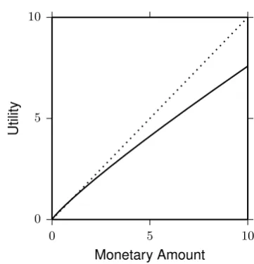
1.1 Example utility function: u(x) = x0.88. Dotted line represents an identity function. Parameter value, 0.88, is taken from Tversky and Kahneman (1992). . . 3

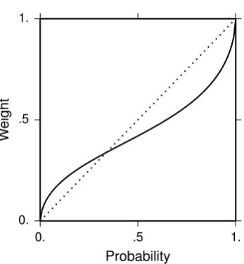
1.2 Example weighting function for prospect theory: w(p) = exp(−1.30 (−log(p))0.55). Dotted line represents an identity function. Functional form is taken

from Prelec (1998), and parameter values are arbitrarily specified to reproduce the weighting function illustrated in Kahneman and Tver-sky (1979). . . 5 1.3 Example weighting function for cumulative prospect theory: π(p) =

p0.61

(p0.61₊₍₁₋_p₎0.61₎0.161

. Dotted line represents an identity function.

Pa-rameter value, 0.61, is taken from Tversky and Kahneman (1992). . 8 1.4 Example preference development. Two lines represent preference for

two alternatives, and dotted line is a response threshold. . . 12 1.5 Illustration of alternatives in multi-alternative choice. Choice

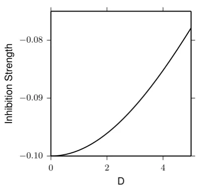
be-tween Cars A and B can be affected by the presence of Car D, C, or S. . . 13 1.6 Example inhibition function: −0.10 exp(−0.01D2). Parameter

val-ues are taken from Hotaling, Busemeyer, and Li (2010). . . 14

2.1 Predicted utility map over a probability triangle. A point in this triangle represent an alternative, whose potential outcomes are £20,

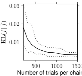
£10, and £0. Probability of £20 is shown on the vertical axis, and probability of£0 is shown on the horizontal axis. . . 21 2.2 The KL divergences between f and ˆf for various numbers of trials.

(9)

2.4 ln( ˆf): logged estimation of utility map. Each panel represents utility map for one participant. Solid line represents indifference line. . . . 28

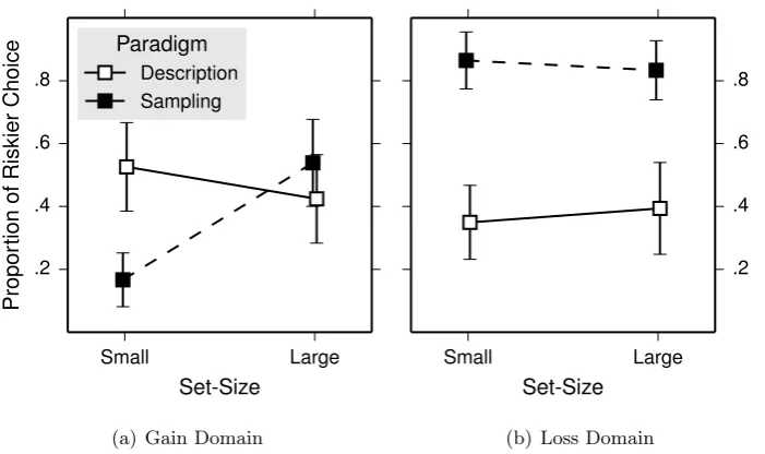
3.1 Example screen-shots. . . 37 3.2 Proportion of choices for riskier alternatives in Experiment 1. Error

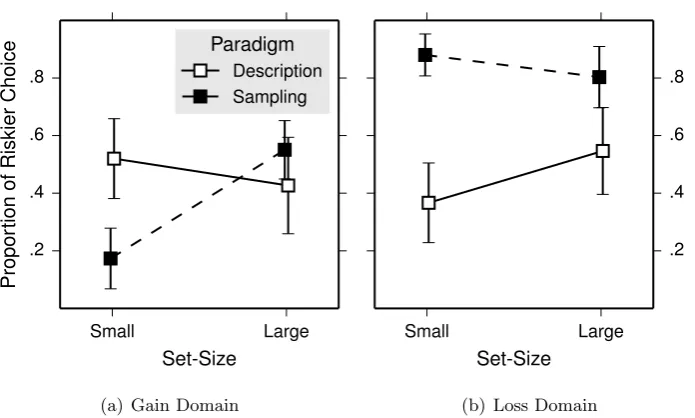
bars are 95% confidence interval. . . 38 3.3 Proportion of choices for riskier alternatives in Experiment 2. Error

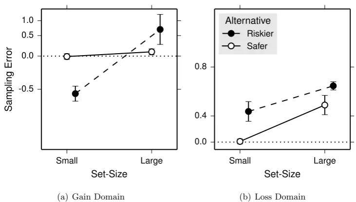
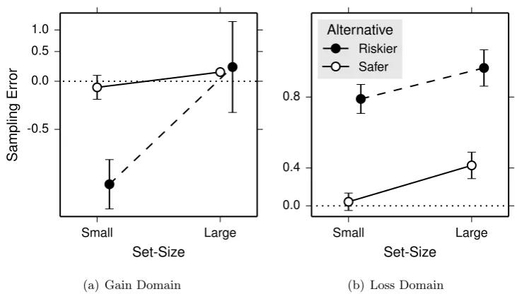
bars are 95% confidence interval. . . 39 3.4 Sampling error in Experiment 1. For illustration purposes, sampling

error is mean-averaged across trials for each participant. Marker in-dicates grand mean and error bars are 95% confidence interval. . . . 40 3.5 Sampling error in Experiment 2. For illustration purposes, sampling

error is mean-averaged across trials for each participant. Marker in-dicates grand mean and error bars are 95% confidence interval. . . . 41 3.6 Sampling error for a riskier alternative against the number of

alterna-tives sampled. Each marker represents a trial, and each participant has up to three entries into the figure. Solid line is predicted sampling error from a mixed-effect linear regression. . . 43 3.7 Simulation results for the gain domain. . . 46 3.8 Simulation results for the loss domain. . . 46

4.1 Proportion of choice deferral. Error bar represents standard error. . 57 4.2 Proportion of alternatives sampled. Error bar represents standard

error. . . 58 4.3 Number of samples per alternative. Error bar represents standard

error. . . 59 4.4 Differences in largest pay-offs in the description paradigm when a

choice was purchased compared to when a choice was deferred. Pay-off in the right panel is normalized. Error bar represents standard error. . . 61 4.5 Differences in maximum mean samples in the sampling paradigm.

Error bar represents standard error. . . 64

(10)

5.2 Simulated choice probability. The darkness of the line corresponds to the likelihood of the attention frequency given the equal weighting, and vertical dotted line represents most likely attention split. The left panel illustrates that when Car D or S is included in a choice set, more sampling of the quality dimension predicts higher probability of Car A to be chosen. The right panel shows that the probability of choosing Car A decreases with the frequency of comparisons between Cars B and D, C, or S. . . 72 5.3 Example screen-shots. This example depicts a choice between cars in

an attraction choice. Font size is enlarged for this illustration. . . 75 5.4 Locations of the alternatives used in the experiment. . . 75 5.5 Mean choice proportions of the engaged participants. Error bars are

standard error of the mean. In the attraction choices, DA is inferior

to A in both attributes, and DB is inferior to B. In the compromise

choices, CA makes A a compromise between the other alternatives,

and CBmakes B a compromise. In the similarity choices, SAis similar

to B and SB is similar to A. The subscript of labels indicate which

alternative (A or B) is favored by the context. . . 77 5.6 Fixation duration as a function of time. Error bars are standard error

of the mean. . . 79 5.7 Difference in transitions. Error bar are standard error of the mean. . 80 5.8 Number of transitions prior to making a choice. Error bars are

stan-dard errors of the mean. . . 83 5.9 Number of transitions prior to making a choice. Error bars are

stan-dard errors of the mean. . . 87

6.1 Attraction choice set. . . 93 6.2 Counts of eye-fixation transition between alternatives. Grey circles,

(11)

6.5 MDbS prediction of the attraction effect. Square and circle markers show prediction with the posterior median parameters, and error bar

represents 95% highest density interval. . . 101

6.6 MDbS prediction of the attraction effect with various locations of Car D, from E to A (endpoint exclusive). The shaded area indicates 95% highest density intervals. . . 102

6.7 MDbS prediction of the attraction effect with various decoys. Error bar represents 95% highest density interval. . . 102

6.8 MDbS prediction of the compromise effect. Square marker shows prediction with the posterior median parameters, and error bar rep-resents 95% highest density interval. . . 103

6.9 MDbS prediction of the similarity effect. Square marker shows predic-tion with the posterior median parameters, and error bar represents 95% highest density interval. . . 104

6.10 Predicted number of comparisons before choosing A, B, or T. . . 105

6.11 Simulated effects of choice familiarity. The square markers in Panels (b), (c), and (d) represents median predictions with the posterior median parameters. Error bars are 95% highest density interval. . . 106

6.12 Simulated effects of display duration. The shaded area represents 95% highest density interval. . . 108

6.13 Perceptual focus effect documents the choice of Car A. . . 108

6.14 Attribute balance effect documents the choice of Car A. . . 109

6.15 Attribute range effect. . . 111

6.16 MDbS posterior predictives for p(Choose A) ₋p(Choose B). The square markers show the prediction with the posterior median pa-rameters (α= 0.056,β0 = 15.01, β1 =−14.65 γ = 0.36, and λ= 3), and the error bars show the 95% highest density interval. The cross represents overall mean. . . 113

6.17 MDFT posterior predictives for p(Choose A)₋p(Choose B). The square markers show the prediction with the posterior median param-eters (φ1 = 2.02, φ2 = 1.01,ξ = 15.39, σ2 = 0.02, and a threshold is 1.89), and the error bars show the 95% highest density interval. The cross represents overall mean. . . 114

6.18 Predictive accuracy of the models. . . 115

(12)

Acknowledgments

I would like to thank Adam Sanborn and Neil Stewart for their supportive

super-vision of this thesis. Their advice and comments were invaluable. I am also very

grateful to Thomas T. Hills, with whom I have collaborated on some of the projects

presented here.

(13)

Declarations

This thesis is submitted to the University of Warwick in support of my application

for the degree of Doctor of Philosophy. It has been composed by myself and has not

been submitted in any previous application for any degree.

The work presented (including data collection and data analysis) was carried

out by the author except in the cases outlined below: Chapter 2 was written in

collaboration with Adam Sanborn and Neil Stewart; Chapters 3 and 4 were

writ-ten in collaboration with Thomas T. Hills; and Chapters 5 and 6 were writwrit-ten in

collaboration with Neil Stewart.

List of publications including submitted papers:

Chapter 2

Noguchi, T., Sanborn, A., & Stewart, N. (2013). Non-parametric estimation of the

individual’s utility map. In M. Knauff, M. Pauen, N. Sebanz, & I. Wachsmuth

(Eds.), Proceedings of the 35th Annual Conference of the Cognitive Science

Society, Austin, TX: Cognitive Science Society.

Chapter 3

Noguchi, T., & Hills, T. T. (submitted). Set-size induced risk-amplification:

Experience-based decisions in large set-sizes favour riskier alternatives.

Noguchi, T., & T. T. Hills. (2014). Context effects and risk amplification: Why

more is risky. In P. Bello, M. Guarini, M. McShane, and B. Scassellati (Eds.),

Proceedings of the 36th Annual Conference of the Cognitive Science Society,

Austin, TX: Cognitive Science Society.

(14)

Noguchi, T., & Hills, T. T. (submitted). Thin-search and choice deferral:

Encour-aging myopic choices with more information.

Chapter 5

Noguchi, T., & Stewart, N. (2014). In the attraction, compromise, and similarity

effects, alternatives are repeatedly compared in pairs on single dimensions.

(15)

Abstract

Behavioral research has long documented that the choices an individual makes do not always follow the maximization of expected values. To describe the utility an individual maximizes through his or her choices, one class of models — static models — has been previously developed. These models are reviewed in Chap-ter 1. To assess the static models, a non-parametric method to reveal the utility of alternatives is developed in Chapter 2. The results show that the utility predicted from the static models deviates from the estimated utility.

Utility, however, is relatively unstable across contexts determined by infor-mation presentation formats, choice set-sizes, the structures of alternatives, and the relationships between alternatives. This instability is a topic for Chapters 3, 4, and 5. Following Chapter 3, which examines effects of information presentation formats and choice set-sizes on risk-taking, Chapter 4 further investigates how the contexts impact on choice evaluation. Then, Chapter 5 examines process of choice evaluation by analyzing eye-movements during choices. The results from these three chapters indicate that choices are systematically altered with contexts, supporting instability of utility.

The instability of utility conflicts with the principle of utility maximization, and Chapters 5 and 6 consider another class of models — dynamic models — which can accommodate utility instability. A dynamic model assumes that an individ-ual iteratively and stochastically develops preferences for each alternative, until preference for one alternative reaches a choice criterion. The exact processes of preference development is investigated in Chapter 5, which suggests that a dynamic model should be based on single-attribute pair-wise comparisons. Following this suggestion, a new model — multi-alternative decision by sampling — is proposed in Chapter 6.

(16)

Chapter 1

Introduction

Choice making lies at the heart of human behavior. When an individual walks across a busy street, the individual is assessing a risk of being run over a car and choosing when to cross the street. When an individual looks through a menu at a restaurant, the individual is evaluating each dish on the menu and choosing which dish he or she prefers the most. Some of choices, such as choosing who to marry with, have life-changing consequences, while others may have more trivial consequences. Studies on how an individual makes those choices has been of great interest for psychologists, economists and researchers in many other field. Psychology of choice has been studied since the 18th century and has attracted increasing attention especially over the last three decades.

This thesis investigates how an individual evaluates an alternative and how he or she makes a choice, and this investigation extensively uses mathematical mod-els to understand choices. There exist numerous mathematical modmod-els to explain a number of phenomena observed with various experimental paradigms, ranging from perceptual choice (e.g., choosing a brighter patch) to consumer choice (e.g., choosing a car to purchase). These mathematical models have been practically and theoretically proved useful, as they can be readily tested with various alternatives and compared against actual choice behavior.

(17)

the models I use throughout the rest of thesis. Thus, this chapter does not aim to provide comprehensive review of the field, but rather, it aims to introduce the models relevant to the chapters to follow.

1.1 Static Models

Choice models, especially those in economics, often assume utility maximization. Here, an individual is assumed to choose an alternative which maximizes utility. Since studies in 18th century, it has been empirically shown that an individual’s choice is not well explained by maximization of expected pay-off. To understand an individual’s choice, various models have been proposed to describe utility of an alternative. I start the review with one of the earliest models: expected utility theory.

1.1.1 Expected utility theory

Expected utility theory was first proposed by Bernoulli (1738/1954) to explain be-havioral phenomena associated with a price an individual should pay to play a gamble. The individual can be assumed to pay any price up to the expected pay-off from the gamble, but violation of this assumption is observed with St. Petersburg game. In this game, a coin is flipped repeatedly until a head is produced. If an individual enters this game, the individual earns pay-off of £2n, where n is the number of coin flips before landing a first head. An expected pay-off from this game is calculated as follows:

∞

X

n=1

1 2n2

n₌

∞

X

n=1

1 =_∞.

If an individual is willing to pay any price up to the expected pay-off, this individual should be willing to pay any price at all: for example, hundreds of pounds.

(18)

0 5 10 Monetary Amount

0 5 10

[image:18.595.227.408.107.295.2]

Utility

Figure 1.1: Example utility function: u(x) = x0.88. Dotted line represents an identity function. Parameter value, 0.88, is taken from Tversky and Kahneman (1992).

the other models, I assume a power function, u(x) = xα, where 0 < α < 1. As an illustration, an utility function withα = 0.88 is displayed in Figure 1.1. Then, expected utility in the St. Petersburg game is calculated as below:

∞

X

n=1

1 2nu(2)

n₌

∞

X

n=1

1 2n(2

α₎n₌

∞

X

n=1

1 2n2

αn₌

∞

X

n=1

2αn−n

<

∞

X

n=1

2n−n=

∞

X

n=1

1 =_∞. (∵α <1)

With a concave utility function, an expected utility in the St. Petersburg game is less than infinity, which predicts that an individual should be willing to pay only up to a finite amount of price to enter this game. Please note however, that utility function is not a general solution, since other pay-off structures could still lead to infinite value in a variant of St. Petersburg game.

1.1.2 Prospect theory

(19)

Allais’s paradox (Allais, 1953).

This paradox is empirically tested by Kahneman and Tversky (1979), where an individual is asked to make a choice between the following two alternatives.

A: 2,500 with probability .33, 2,400 with probability .66, 0 with probability .01;

B: 2,400 with certainty.

Kahneman and Tversky (1979) report that 82% of individuals chose Alternative B over A. Kahneman and Tversky (1979) also tested the following two alternatives:

C: 2,500 with probability .33, 0 with probability .67;

D: 2,400 with probability .34, 0 with probability .66.

These alternatives are obtained by eliminating a .66 probability of 2,400 pay-off from Alternatives A and B, and hence, ordering of expected utility should not be affected: if Alternative B is chosen over A, Alternative D should be chosen over C. However, 82% of individuals chose Alternative C over D. This pattern of behavior indicates violation of expected utility theory.

According to expected utility theory, the choice of Alternative B over A implies the following:

.33u(2,500) +.66u(2,400)< u(2,400),

which is equivalent to

.33u(2,500)< .34u(2,400).

The left term of this inequality corresponds to Alternatives C, and the right term corresponds to D. Thus, expected utility theory predicts that if Alternative B is chosen over A, Alternative D should be chosen over C. This prediction is violated in the observation by Kahneman and Tversky (1979), where Alternative C is more frequently chosen than D.

Prospect theory resolves this paradox and several other violations of expected utility theory with editing rules and a weighting function. The editing rules pre-process probabilities and pay-offs of an alternative before applying the utility and the weighting functions. To resolve Allais’s paradox however, only the weighting function is required. With the weighting function, w, choice of Alternative B over A implies:

(20)

0. .5 1. Probability

0. .5 1.

W

eight

Figure 1.2: Example weighting function for prospect theory: w(p) = exp(−1.30 (−log(p))0.55). Dotted line represents an identity function. Functional form is taken from Prelec (1998), and parameter values are arbitrarily specified to reproduce the weighting function illustrated in Kahneman and Tversky (1979).

which is equivalent to

w(.33)u(2,500)<(1₋w(.66))u(2,400).

Also, choice of Alternative C over D implies

w(.34)u(2,400)< w(.33)u(2,500).

Thus if an individual chooses Alternative B over A and Alternative C over D, these choices implies

w(.34)u(2,400)<(1₋w(.66))u(2,400),

or

w(.34)<1−w(.66).

More generally, prospect theory is able to resolve Allais’s paradox, as long as the following condition holds:

(21)

This condition is satisfied by having a non-linear weighting function. Kahneman and Tversky (1979) do not provide a functional form for a weighting function, but Prelec (1998) examined several forms of a weighting function. An example is illustrated in Figure 1.2. Mathematical proof that this particular weighting function satisfies Equation 1.1 is provided by Prelec (1998).

Thus with the editing rules and a non-linear weighting function, prospect theory is able to explain Allais’s paradox and various other behavior (see Kahneman & Tversky, 1979, for details), which expected utility theory is not able to explain. Also as prospect theory has an utility function u as expected utility theory does, prospect theory predicts that subjective value of the St. Petersburg game is finite.

1.1.3 Cumulative prospect theory

One major limitation of prospect theory, however, is that it potentially permits violation of stochastic dominance. Suppose an individual is making a choice between Alternatives E and F:

E: x1 with probability p1,

x2 with probability p2,

0 with probability 1−p1−p2;

F: x1 with probability p01,

0 with probability 1−p0₁−p0₂. Further assume that

0< x1< x2,

p0₂< p2, and

p1+p2=p01+p02 <1.

(1.2)

Then, Alternative E dominates F: Alternative E has a higher probability of obtaining a larger pay-off, x2, than Alternative F, and also E has the same probability of

obtaining the worse pay-off, 0, as F. Thus, Alternative E should be chosen over F, which implies

w(p0₁)u(x1) +w(p02)u(x2)< w(p1)u(x1) +w(p2)u(x2),

or

u(x1)

u(x2)

< w(p2)−w(p

0

2)

w(p0₁)₋w(p1).

(1.3)

(22)

E’: x1 with probability p02,

0 with probability 1₋p0₂₋p0₁;

F’: x1 with probability p2,

0 with probability 1₋p2−p1.

Alternative E’ dominates F’, because Equation 1.2 indicates p1 < p01: Alternative

E’ has a higher probability of obtaining a larger pay-off than Alternative F’. Also, Alternative E’ has the same probability of obtaining the worst pay-off as Alternative F’. Then, choice of Alternative E’ implies the following:

w(p2)u(x1) +w(p1)u(x2)< w(p02)u(x1) +w(p01)u(x2),

or

u(x1)

u(x2)

< w(p

0

1)−w(p1)

w(p2)−w(p02).

(1.4)

Asx1 becomes similar to x2, the left term in Equations 1.3 and 1.4 approaches to

1. Thus, satisfaction of Equations 1.3 and 1.4 implies:

1_≤ w(p2)−w(p

0

2)

w(p0₁)₋w(p1)

and 1_≤ w(p

0

1)−w(p1)

w(p2)−w(p02)

⇔ 1≤ w(p2)−w(p 0

2)

w(p0₁)−w(p1)

and 1≥ w(p2)−w(p 0

2)

w(p0₁)−w(p1)

⇔ 1 = w(p2)−w(p

0

2)

w(p0₁)₋w(p1)

⇔ w(p1) +w(p2) =w(p01) +w(p02)

However,w(p1) +w(p2) cannot be the same asw(p01) +w(p02), as wis a non-linear

function and p1+p2 =p10 +p02 is assumed (Equation 1.2). Thus when x1 is very

close to x2, prospect theory eventually violates Equation 1.3 or 1.4, predicting a

choice of the dominated alternative.

This limitation is overcome with cumulative prospect theory (Tversky & Kahneman, 1992), which employs a cumulative weighting function. Suppose an alternative is associated with a pi probability of xi pay-off, where i = 1,2, . . . , n.

Whenxi < xj for alliandjwhich satisfy 1≤i < j≤n, then a weight is computed

as follows:

w(pi) = π( n

X

j=i

pj)−π( n

X

j=i+1

(23)

0. .5 1. Probability

0. .5 1.

W

[image:23.595.235.409.106.294.2]

eight

Figure 1.3: Example weighting function for cumulative prospect theory: π(p) =

p0.61

(p0.61₊₍₁₋_p₎0.61₎0.161

. Dotted line represents an identity function. Parameter value,

0.61, is taken from Tversky and Kahneman (1992).

and

w(pn) = π(pn).

With this cumulative weighting function, the right term in Equation 1.3 becomes the following:

w(p2)−w(p02)

w(p0₁)−w(p1)

= π(p2)−π(p

0

2)

π(p0₂+p0₁)−π(p₂0)−π(p2+p1) +π(p2)

= π(p2)−π(p

0

2)

−π(p0₂) +π(p2)

(∵p2+p1 =p02+p01)

= 1

> u(x1) u(x2)

(_∵x2> x1).

Thus, cumulative prospect theory satisfies both Equations 1.3 and 1.4, and hence stochastic dominance, independent of exact expression ofπ.

To explain choice better, however, Tversky and Kahneman (1992) proposes the following functional expression forπ:

π(p) = p

γ

(pγ_{+ (1}₋_p₎γ₎γ1

.

(24)

typical risk-seeking for a small probability. An individual tends to overweight small probabilities and underweight high probabilities, so that this individual often chooses an alternative with a small probability of large pay-off over an alternative with a high probability of small pay-off. Also when this weighting function is linear, cumulative prospect theory becomes identical to expected utility theory. Thus, cumulative prospect theory can be seen as a general case of expected utility theory. Performance of cumulative prospect theory is compared against performance of expected utility theory in Chapter 2, and also an extension of cumulative prospect theory is used in simulations in Chapter 3.

1.1.4 Transfer of attention exchange model

More recent empirical studies, however, report notable violation of cumulative prospect theory (see Birnbaum, 2008, for review). Here, I review only one of such violations: violation of coalescing. In one of the experiments reported by Birnbaum (2008), an individual made a choice between the following two alternatives:

G: 100 with probability .85, 50 with probability .15;

H: 100 with probability .95, 7 with probability .05.

The majority of individuals choose Alternative G over H. However, when confronted with the following two alternatives, the majority of individuals choose Alternative H’ over G’.

G’: 100 with probability .85, 50 with probability .10, 50 with probability .05;

H’: 100 with probability .85, 100 with probability .10, 7 with probability .05.

Alternative G is a coalesced form of Alternative G’. The pay-off of 50 with a proba-bility of.15 in Alternative G is split into the two possible pay-off of 50 in Alternative G’. Similarly, the pay-off of 100 with a probability of.95 is split into the two pos-sible pay-offs in Alternative H’. In cumulative prospect theory, split pay-offs are automatically coalesced because of cumulativity of a weighting function, and thus, cumulative prospect theory predicts that if an individual chooses Alternative G over H, this individual should choose G’ over H’. The violation is also reported by Birnbaum (1999).

To explain violation of coalescing, Birnbaum and Chavez (1997) propose transfer of attention exchange model. Suppose an alternative is associated with api

probability ofxi pay-off, wherei= 1,2, . . . , n. When xi < xj for alli and j which

(25)

subjective value of this alternative is computed as follows:

Pn

i=1t(pi)u(xi) +Pni=1

Pn

k=i(u(xi)−u(xk)) ω(pi, pk, n)

Pn

i=1t(pi),

wheretis a weighting function, t(p) =pγ, and

ω(pi, pk, n) =

     

    

δ t(pk)

n+ 1 δ >0,

δ t(pi)

n+ 1 δ≤0.

The weight transfer function, ω, determines how much attention transfers from a better possible pay-off to a worse pay-off, where attention transfer is specified by parameterδ.

This transfer of attention exchange model does not coalesce pay-offs, and as a result, the model predicts different subjective values for Alternatives G than G’. As Alternative G has only one worse pay-off of 50 and Alternative G’ has two, less attention transfers to 50 pay-off for Alternative G than G’. Thus, the coalescing makes Alternative G better than G’. Similarly, coalescing makes Alternative H worse than H’, because more attention transfers from a better pay-off of 100 for Alternative H than for H’.

The transfer of attention exchange model explains Allais’s paradox with transfer of attention. When evaluating the following alternatives,

A: 2,500 with probability .33, 2,400 with probability .66, 0 with probability .01;

B: 2,400 with certainty,

attention transfers from pay-offs of 2,500 and 2,400 to pay-off of 0 in Alternative A. As a result, subjective value for Alternative A is less than subjective value for Alternative B. When 2,400 with probability.33 is subtracted from each Alternative, however, attention transfers to pay-off of 0 in both alternatives:

C: 2,500 with probability .33, 0 with probability .67;

D: 2,400 with probability .34, 0 with probability .66.

As a result, the difference in the pay-offs of 2,500 and 2,400 carries over to the dif-ference in subjective values of alternatives: Alternative C is predicted to be chosen by the transfer of attention exchange model.

(26)

finding that an individual prefers a pay-off with probability 1.0 over a probabilistic pay-off with the same or even higher expected pay-off. An example is the following two alternatives:

K: 2,500 with probability 1.00; L: 5,000 with probability .50, 0 with probability .50.

Majority of individuals prefers Alternative K over L. This risk aversion is ex-plained with a concave utility function in expected utility theory, which predicts that u(2,500)_×1.0 > u(5,000)_×0.5. Similar explanation is provided by the con-cave utility function together with the weighting function in prospect theory and cumulative prospect theory.

The transfer of attention exchange model, however, explains risk aversion with attention transfer: in Alternative L, attention transfers from 5,000 pay-off to 0 pay-off, resulting in less weight on 5,000 than.50. Thus with the identity utility function, the transfer of attention exchange model predicts that the subjective value of Alternative L is less than 5,000_×0.5 = 2,500, which is the subjective value of Alternative K. The same mechanism predicts finite subjective value for the St. Petersburg game. As the transfer of attention exchange model can explain more choice phenomena, this model can be more flexible than other models.

Performance of the transfer of attention exchange model is assessed and compared against performance of expected utility theory and cumulative prospect theory in Chapter 2.

1.2 Dynamic Models

In contrast to static models, which have been developed in a domain of economic choice, dynamic models were initially developed with perceptual identification tasks. An example perceptual task presents two sequences of alphabetical characters and ask an individual to respond “yes” if the two sequences are both words or both non-words and “no” otherwise (Meyer & Irwin, 1981). To explain speed and accuracy of such judgment, models have been developed with an idea that after presentation of stimuli, an individual sequentially evaluates and accumulates information from the stimuli. When the accumulated information reaches a response criterion, the individual is assumed to make a judgment (e.g., respond with “yes” or “no”).

(27)

Start Choice Time

0

Pref

erence

Figure 1.4: Example preference development. Two lines represent preference for two alternatives, and dotted line is a response threshold.

infinite amount of time in making a judgment. However, it typically takes much less than a second to identify a perceptual stimulus (e.g., Ratcliff, 1978), indicating a trade-off between speed and accuracy of judgment. As a result, dynamic models often provide an account for process of judgment, while static models typically do not provide such an account.

Over the last five decades, various dynamic models have been proposed and successfully explained speed-accuracy trade-offs in various perceptual judgments (e.g., Stone, 1960; Ratcliff, 1978; see Bogacz, Usher, Zhang, & McClelland, 2007 for review). Following these success, dynamic models have been extended to provide a unifying framework to explain economic choices. When applied to economic choice, a dynamic model is considered to be a model of preference development. The mo-ment an individual faces alternatives, the individual may not have preference for an alternative over another. Rather, the individual is expected to sequentially evaluate alternatives and develop preference for each alternative.

(28)

Economy

Quality A

B D

[image:28.595.236.400.109.278.2]

S C

Figure 1.5: Illustration of alternatives in multi-alternative choice. Choice between Cars A and B can be affected by the presence of Car D, C, or S.

1.2.1 Decision field theory

One of the most well-known dynamic models is decision field theory (Busemeyer & Townsend, 1993). The process implemented in decision field theory is as follows. When confronted with several alternatives to choose from, an individual tries to evaluate all of the attributes associated with each alternative. Values across mul-tiple attribute dimensions cannot be evaluated at the same time, and hence, the individual undergoes a slow and time-consuming process of evaluating, comparing, and integrating the comparisons on single attribute dimension at one time. No choice is made until the preference for one alternative becomes strong enough to guide the individual into choice. Decision field theory successfully explains various phenomena in choice between two alternatives, including those reviewed under static models (see Busemeyer & Townsend, 1993, for details).

To explain choice between three alternatives, decision field theory has been extended to multi-alternative decision field theory (MDFT; Roe, Busemeyer, & Townsend, 2001). In particular, MDFT is developed to provide an unifying ex-planation for the attraction, compromise, and similarity effects. These three effects document that choice can depend on the context determined by the available al-ternatives. An example choice between cars is illustrated in Figure 1.5. Here, each car is described in terms of two attributes, economy and quality. In this example, whether an individual chooses Car A or B can depend on the presence of Car D, C, or S in a choice set. These context effects are discussed in more detail in Chapters 5 and 6.

(29)

0 2 4 D

−0.10 −0.09 −0.08

Inhibition

[image:29.595.223.419.104.289.2]

Strength

Figure 1.6: Example inhibition function: −0.10 exp(−0.01D2). Parameter values are taken from Hotaling, Busemeyer, and Li (2010).

depends on its relationships with other alternatives. Thus for a dynamic model to explain the context effects, a model needs to allow preference for an alternative to impact on preference for another alternative. In this vein, MDFT lets the devel-oping preferences inhibit each other: increasing preference for an alternative causes preference for another alternative to decrease over time. Strength of such inhibition depends on the distance between alternatives, with more similar alternatives more strongly inhibiting each other (Tsetsos, Usher, & Chater, 2010).

To describe computational details of MDFT, I label three alternatives asA,

B, andT, and denote the economy dimension asE and the quality dimension asQ. The value of AlternativeA on the economy dimension is denoted as AE and that

on the quality dimension isAQ. Preference for the three alternatives is organized in

a column vector, P. The first element in this vector corresponds to preference for Alternative A, the second corresponds to preference for B, and the third corresponds to preference for T. This preference is iteratively updated as follows:

P(t+ 1) =S P(t) +V(t+ 1),

whereS is a 3_×3 feedback matrix andV is a 3_×1 momentary valence vector. In the feedback matrix, the influence of AlternativeA onB is computed as:

−φ2 exp(−φ1DAB2 ).

(30)

weighted sum of distance along two orthogonal vectors:

DAB =

(AE−AQ−BE+BQ)2

2 +ξ

(AE+AQ−BE −BQ)2

2 .

Also, the self feedback is computed as 1−φ2. An example inhibition function is

plotted in Figure 1.6. As a distance between alternative, D, increases, inhibition strength moves closer to 0, indicating that preference for one alternative affects the other to a less extent. This distance function is a crucial component for MDFT to explain the attraction, compromise and similarity effects (Tsetsos et al., 2010).

The momentary valence vector is computed with four matrices:

V(t) =C M W(t) +C (t), (1.5)

where

C= 

 

1 ₋1/2 ₋1/2

−1/2 1 −1/2

−1/2 ₋1/2 1   , M =   

AE AQ

BE BQ

TE TQ



 ,

and

(t)_{∼ N}       0 0 0   ,   

σ2 ₀ ₀

0 σ2 0 0 0 σ2

     .

Here, the matrixC indicates that an attribute value of a car is evaluated in relation to the mean average values of the other cars, and indicates that the evaluation is rather noisy. As parameter value for σ increases, the evaluation becomes noisier. The attention weight W is a 2_×1 vector. There is a .50 probability that

W(t) = "

1 0 #

(31)

and also a.50 probability that

W(t) = "

0 1 #

. (1.7)

Equations 1.6 and 1.7 indicate which dimension is attended at given moment. When

W is specified as Equation 1.6, the first dimension, the economy of cars, is attended and the three cars are evaluated according to Equation 1.5. Thus, these equations specify the process where each car is evaluated, for example, on the economy di-mension at one moment, then on the quality didi-mension at next moment, again on the quality dimension at next moment, and so on.

At first, preference for each car is 0, and each car is iteratively evaluated, and when the highest preference reaches the threshold, the alternative is chosen. MDFT has been reported to provide a better fit to empirical choice data than probit regressions which use attribute values to predict choice (Berkowitsch, Scheibehenne, & Rieskamp, in press).

1.2.2 Comparison-grouping model

While multi-alternative decision field theory successfully explains the attraction, compromise, and similarity effects, various other dynamic models have been pro-posed to explain the same effects without clear indication on which model provides better explanations for actual choice behavior.

Here, I review comparison grouping model (Tsuzuki & Guo, 2004). In con-trast to multi-alternative decision field theory, which assumes stochastically fluc-tuating attention over attribute dimensions, comparison grouping model assumes stochastically fluctuating attention over alternatives. At one moment, an individual attends two or three alternatives in a choice set and develops preference for the alternatives.

As an illustration, I again label three alternatives asA,B, andT, which are described with two attributes,E (economy) andQ(quality). The value of Alterna-tiveAon the economy dimension is denoted asAEand that on the quality dimension

is AQ. In the comparison grouping model, each alternative and each attribute

di-mension iteratively develops preference. I denote preference for Alternative A as

PA. Then,

(32)

If Alternative A is not attended at timet+ 1, ∆A(t+ 1) is 0, otherwise

∆A(t+ 1) =

(

ζA(1−PA(t))−λ PA(t) ifζA>0

ζAPA(t)−λ PA(t) ifζA≤0,

(1.9)

where parameterλreflects how much preference decays over time, and

ζA=WAEPE(t) +WQAPQ(t)−τ(PB(t) +PT(t)), (1.10)

and

WAE =

(ln(AE +µ)−ν)

ψ.

Here,WAE determines a weight given to the economy dimension for Alternative A,

which is multiplied by preference for the economy dimension,PE. Also, parameterτ

controls strength of inhibition. As with multi-alternative decision field theory, com-parison grouping model allows preference for an alternative to impact on preference for another alternative. Preference for the other alternatives is updated in the same manner.

In addition, preference for attribute dimensions is updated at each iteration:

PE is updated using Equations 1.8 and 1.9, but instead of Equation 1.10, we have

δE =WAEPA(t) +WBEPB(t) +WTEPT(t).

Thus, preference for the economy dimension is updated to be an average of prefer-ences for the alternatives, weighted by each alternative’s weight given to the economy dimension. Preference for the quality dimension is updated in the similar manner. The iteration is initiated with preference for attribute dimensions and for alterna-tives starts with a random sample from the uniform distribution between 0.25 and 0.75. After 100 iterations, the alternative with the highest preference is chosen.

Given the process above, preference development crucially depends on prob-ability that each alternatives is attended. If one alternative is more frequently attended, this alternative is more likely to develop preference and hence is more likely to be chosen. The probability of attention, however, is manually specified in Tsuzuki and Guo (2004), and its mathematical specification is not available in a way to apply the model to arbitrary sets of alternatives.

(33)

decision field theory. These models are tested in Chapter 5.

1.2.3 Decision by sampling

The last model to be reviewed in this chapter is decision by sampling (Stewart, Chater, & Brown, 2006). Unlike the other dynamic models reviewed above, decision by sampling is developed primarily to explain choice between two alternatives with probabilistic pay-offs and has not been extended to explain the context effects. The extension is proposed in Chapter 6.

In decision by sampling (Stewart et al., 2006), the evaluation of an alter-native on a particular attribute dimension follows the rank position in a sample of attributes, and the rank position is stochastically, iteratively constructed through a series of comparisons. As an illustration, suppose an individual is making a choice between cars. The individual may attend to economy of cars at one moment and compares a car against another car in his or her memory. If the comparison fa-vors the car in a choice set, the individual develops preference for the car. After this comparison, the decision maker may attend another attribute dimension (e.g., quality) at the next moment and makes a comparison. This iterative comparison is repeated until the preferences for the available alternatives are sufficiently different. Here, an alternative is compared against a sample from memory on single attribute dimension at one time. Also, the preference development in decision by sampling is insensitive to the magnitude of the difference. Rather, the preference is proportional to the frequency count of the number of favorable comparisons. The ranks derived in this way replicate a number of empirical findings: for instance, the concave utility function and loss aversion (Stewart et al., 2006). The decision by sampling also provides a reasonable explanation of choice with two alternatives, especially compared against various static models (Stewart & Simpson, 2008).

(34)

to the relative preference for the risky lottery. Similar results are reported on riskless choices: for example, a choice between job applicants (Mellers & Cooke, 1994) and apartments (Cooke & Mellers, 1998). These studies show that, for example, the individuals who frequently saw monthly rents between $350 and $400 find the rent of $350 much more attractive than $400.

1.3 Plan of thesis

(35)

Chapter 2

Non-parametric estimation of

the individual’s utility map

2.1 Background

Understanding how people trade off risk and reward is a fundamental goal of be-havioral economics. The most common approach to modeling how people make decisions between risky alternatives is based on the idea of utility: individuals inte-grate their subjective probability of reward with their subjective value of the reward to produce a single value, their utility that describes how well the alternative is pre-ferred. The utilities of the alternatives are then compared and the alternative with the highest utility is most often chosen.

The normative calculation of utility that maximizes long-term gain is to mul-tiply the probability with the subjective value of the associated outcome. For an illustration, suppose an individual is considering a choice alternative with three possible outcomes: £20, £10, and £0. This particular alternative has a 20% probability for £20, 40% for £10, and 40% for £0. Then, the expected utility is 20%_×v(£20) + 40%_×v(£10) + 40%_×v(£0), wherev is the function to map the monetary value to the subjective value.

(36)

.2 .4 .6 .8 Probability of £0 .2 .4 .6 .8 Probability of £20

(a) The expected utility theory with the identity value function

.2 .4 .6 .8

Probability of £0 .2 .4 .6 .8 Probability of £20

(b) The cumulative prospect theory with parameters α = 0.88 andγ= 0.52

.2 .4 .6 .8

Probability of £0 .2 .4 .6 .8 Probability of £20

(c) The transfer of attention ex-change model with parameters

β= 1,γ= 0.7, andδ= 1

Figure 2.1: Predicted utility map over a probability triangle. A point in this triangle represent an alternative, whose potential outcomes are £20, £10, and£0. Proba-bility of £20 is shown on the vertical axis, and probability of £0 is shown on the horizontal axis.

alternatives with varying probabilities for the same set of three potential outcomes. Throughout this chapter, we use£20,£10, and£0 as the potential outcomes from a choice alternative.

Figure 2.1 displays the predicted utility maps from three of the most well-known models of risky choice: expected utility theory, cumulative prospect theory (Tversky & Kahneman, 1992) and transfer of attention exchange (TAX) model (Birnbaum, 2008). The differences between the models can be seen in the shapes of the indifference lines. Expected utility theory predicts indifference lines that are parallel and straight. Cumulative prospect theory predicts lines that are concave where the probability of the best outcome is larger than that of the worst outcome, but convex lines where the probability of the best outcome is less than that of the worst. The TAX model predicts indifference lines that are convex throughout the triangle.

The usual experimental practice is to investigate choices in regions of the triangle where models most differ from each other (e.g., Wu & Gonzalez, 1998). When the models are tested in this way, the best model may not predict choices away from the diagnostic regions well. For instance, Harless (1992) reports that the cumulative prospect utility explains choice better than the expected utility theory only in the boundary region of the triangle.

(37)

modified MCMC with People to investigate regions of the probability triangle where the choice alternatives are less preferred. The new method is tested in a simulation to show that it can deliver useful results within a reasonable number of trials. We then estimate utility maps from human data and determine which model fits best. Finally, we discuss the results and future applications for this approach.

2.1.1 Markov chain Monte Carlo with People

Markov chain Monte Carlo (MCMC) is a common method for drawing samples from a distribution. It has been widely used to draw probabilistic inference espe-cially when solving the exact function of interest is computationally difficult (Neal, 1993). Samples drawn with MCMC are typically used to make an inference on the distribution, and here, we use samples to infer the shape of utility map over the triangle.

MCMC begins in a start state z. Then a sample z0 is first drawn from the proposal distribution q, then z0 is evaluated with the function of interest,π to de-termine whether to accept z0 as a new state or discard it and retain the current state z. The sequence of accepted samples forms a Markov chain, and after this Markov chain converges, accepted samples can be regarded as samples fromπ dis-tribution. To ensure that the Markov chain converges to π, detailed balance needs to be satisfied

π(z)q(z0|z)A(z0, z) =π(z0)q(z|z0)A(z, z0), (2.1)

whereq(z0_|z) is the probability of drawingz0 when the current state iszandA(z0, z) is the probability of accepting proposalz0 over the current state z.

Throughout the chapter, we assume a symmetric distribution forq,q(z0_|z) =

q(z_|z0), so Equation 2.1 becomes

π(z)A(z0, z) =π(z0)A(z, z0). (2.2)

Detailed balance can be satisfied by carefully designing the acceptance func-tion A. The most commonly used function is the Metropolis acceptance function (Metropolis, Rosenbluth, Rosenbluth, Teller, & Teller, 1953), but the Boltzmann acceptance function (Flinn & McManus, 1961) is of interest here:

A(z0, z) = π(z

0₎

π(z) +π(z0).

(38)

is because the Boltzmann function is equivalent to Luce’s choice rule (Luce, 1959), which has been frequently used to model risky choice (e.g., Loomes & Sugden, 1998; Blavatskyy & Pogrebna, 2010). As a result, by sequentially presenting pairs of choice alternatives to an individual (where the new alternative z0 is selected by the computer), the collection of choice alternatives chosen by the individual can be treated as samples from the probability distribution whose density is proportional to the individual’s utility.

2.1.2 Extending MCMC with People

However, samples from the individual’s utility distribution does not necessarily serve to estimate the shape of the utility map: pilot work confirms that all of the samples will be concentrated around the most favorable alternative (100% probability of

£20 in the triangle), leaving the rest of the utility map unexplored. To enable the reasonable estimation of the utility map, the Markov chain has to travel better around the triangular space.

For this purpose, we implement a latent agent in the experimental program. This latent agent makes an independent choice between the same alternatives as participant, and only when the agent and participant both select the new choice al-ternative, the new alternative becomes the new state. Otherwise, the current state remains the same and another alternative is generated from the proposal distribu-tion.

When the agent is implemented in this way, the acceptance function be-comes a joint function of the participant’s and the agent’s choices. Specifically, the acceptance function is defined as

A∗(z0, z) = f(z

0₎

f(z) +f(z0₎

g(z0)

g(z) +g(z0₎_,

wheref is the utility function for participant and g is the agent’s utility function. Here, both participant and the agent follow the Boltzmann acceptance function. Then Equation 2.2 becomes

f(z)g(z)A∗(z0, z) =f(z0)g(z0)A∗(z, z0).

(39)

this extended method, the stationary distribution of the Markov chain is the joint utility function of the participant and the agent,f g. Participant’s utility map can subsequently be recovered by dividing the joint utility by the latent agent’s known utility.

2.2 Simulation

To demonstrate that the developed method can estimate a participant’s utility map within a reasonable number of trials, a simulation was run. The simulation used the two of the utility functions in Figure 2.1: g was set to the inverse of expected utility theory, andf was cumulative prospect theory. The proposal distribution, q, was uniform over the triangular space. The possible outcomes were fixed to be£20,

£10 and £0.

With these functions, a choice trial was simulated as follows. First, the agent used thegfunction to evaluate each alternative and uses the Boltzmann acceptance function to select between the current state and the proposed alternative. If the agent preferred the current state over the proposed alternative, another alternative was sampled from the proposal distribution. If the latent agent chose the new alternative over the current state, the virtual participant withf function then made a choice between the same two alternatives.

Although the agent and the virtual participant could have made a choice at the same time over the same two alternatives, we had the agent decide first: if the agent does not select the new alternative, the previous state remains the state regardless of the choice the participant makes. This reduces the number of choices the participant must make.

Each simulation consisted of three chains: one chain started with the Markov state of 60% of £20, 20% of £10 and 20% of £0. Another chain started with the state of 20% of £20, 60% of £10 and 20% of £0 as the starting state. The final chain started with 20% of£20, 20% of £10 and 60% of £0.

(40)

500 1000 1500

Number of trials per chain

0.01 0.02 0.03

K

L

(

f

||

[image:40.595.248.391.107.239.2]

ˆ_f)

Figure 2.2: The KL divergences between f and ˆf for various numbers of trials. The solid line represents the mean measurement of the 10 simulation runs, and the dotted lines are maximum and minimum values archived in the simulations.

produced less bias than other alternatives. The Dirichlet kernel is defined as

ˆ

f(x)g(x) =X

i

Dir(zi|α1, α2, α3),

wherezi is theith state in the Markov chain,xis a vector of probabilities for three

outcomes, andαj isxj/min(h, xj,1−xj). The kernel widthh was set to 0.09. This

smoothed joint distribution is then divided byg to derive the estimation ˆf.

To assess the similarity between f and ˆf, we computed Kullback–Leibler (KL; denoted as KL(f_||fˆ)) divergence (Kullback & Leibler, 1951), which measures how much information is lost in the estimation process. The KL divergences for different sample sizes are plotted in Figure 2.2. This figure illustrates that the estimation shows the increasingly smaller divergence within the first few hundred trials. The estimation becomes reasonably accurate on average after 700–800 trials. The two panels of Figure 2.3 display the estimations after 1,000 trials. The estimation with the smallest KL divergence among the 10 simulation runs is in the left panel, and the right panel show the estimation with the largest KL divergence. Both panels show the key properties of the cumulative prospect theory: the es-timated maps display the concave indifference lines where the probability of £20 is greater than the probability of £0, and the indifference lines are convex in the other area. Also, the indifference lines show fanning-out property from the lower left corner toward the diagonal boundary.

(41)

(a) The estimation with the smallest KL divergence (KL(f||fˆ) = 0.002)

(b) The estimation with the largest KL divergence (KL(f||fˆ) = 0.007)

Figure 2.3: Estimation of the cumulative prospect theory with 1,000 trials

2.3 Experiment

2.3.1 Method

Participant

Ten participants were recruited through the subject panel at the University of War-wick. One participant did not complete the experiment, leaving nine (five male and four female) participants. Their age ranged from 19 to 30 with a mean of 22.9.

Procedure

The experimental procedure closely followed that of the simulation. Three chains with the same start states were run interleaved until participants had made 1,000 choices per chain. In each trial, the latent agent made a decision first, and a new alternative was drawn from the uniform distribution over the entire triangle until the agent chose the new alternative. The latent agent’s utility function was set to be the prediction from the expected utility theory raised to the power of−8, which was enough to ensure coverage of the map in pilot work.

In addition, 50 catch trials were inserted to the experiment, so that we could assess whether participants were engaged in the task. In each catch trial, one al-ternative had larger probabilities for both £20 and £10. If a participant was not engaged with the task and randomly making choices, it is expected that he or she would occasionally not select the non-dominant alternative.

(42)

the online experiment and take a break after spending one hour on it. After the minimum break of three hours, participants were allowed to log in again and resume the experiment.

The choices participant made were incentivized: we invited participants to the lab when participants completed the experiment. At the lab, we randomly selected one trial from the experiment and played the selected alternative for real. Participants were paid what they earned from the play.

2.3.2 Result and Discussion

All the participants selected the dominant alternative in all of the catch trials, which was evidence that all participants understood and were engaged in the task.

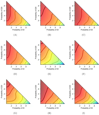
Utility maps were estimated as in the simulation study. All participants show a sharp peak at the top corner of the triangle in the estimated maps. The sharp peak makes it difficult to see the shape of the map, and thus for illustration purposes, we spaced out the indifference lines by taking the natural logarithm of the estimation. As a result, small differences in utility are exaggerated, but the shapes of the indifference lines are not affected. The resulting maps are displayed in Figure 2.4. Each panel in the figure corresponds to one participant’s map.

The estimated maps show the steep indifference lines, especially where the probability of£0 is small. The steep lines indicate aversion to the worst outcome (c.f., Brandstatter, Gigerenzer, & Hertwig, 2006), where the increment in proba-bility for the worst outcome needs to be compensated with a larger increment in probability for the most desirable outcome. The steepness tends to be lessened near the lower right corner of the triangle. As a result, for Participants A, D and H in particular, the indifference lines show the fanning-out property. The fanning-out suggests that participants more willingly accept an increment in probability for the worst outcome when the probability is already large. The fanning-out is consistent with the prediction from the cumulative prospect theory.

(43)

.2 .4 .6 .8 Probability of £0 .2 .4 .6 .8 Probability of £20 (A)

.2 .4 .6 .8

Probability of £0 .2 .4 .6 .8 Probability of £20 (B)

.2 .4 .6 .8

Probability of £0 .2 .4 .6 .8 Probability of £20 (C)

.2 .4 .6 .8

Probability of £0 .2 .4 .6 .8 Probability of £20 (D)

.2 .4 .6 .8

Probability of £0 .2 .4 .6 .8 Probability of £20 (E)

.2 .4 .6 .8

Probability of £0 .2 .4 .6 .8 Probability of £20 (F)

.2 .4 .6 .8

Probability of £0 .2 .4 .6 .8 Probability of £20 (G)

.2 .4 .6 .8

Probability of £0 .2 .4 .6 .8 Probability of £20 (H)

.2 .4 .6 .8

[image:43.595.124.514.173.622.2]

Probability of £0 .2 .4 .6 .8 Probability of £20 (I)

(44)

Thus we approximate the divergence with a Monte Carlo calculation:

KL( ˆf_||model) = Z

p(u_|fˆ)_{ln(p(u_|fˆ))₋ln(p(u_|model))_}du

≈ 1

n

X

i=1

{ln(p(ˆui|fˆ))−ln(p(ˆui|model))}

≈ 1_n{ln(p( ˆU_|fˆ))₋ln(p( ˆU_|model))_},

where ˆui is theith element in a vector ˆU ofnindependent samples from ˆf. We used

104 asn. The marginal likelihood is computed as follows:

p( ˆU_|model) = Z

p( ˆU_|θ, model)p(θ_|model)dθ.

Here θ is the model parameters, and p(θ|model) is the prior probability of θ. The prior was the uniform distribution between 0 and 2 for all the parameters. This marginal likelihood penalizes unnecessary model complexity (Myung & Pitt, 1997), and thus the KL divergence computed with the marginal likelihood also penalizes unnecessary model complexity.

To allow the predicted maps to adjust the spacing between the indifference lines, the parameter vectorθincludes one additional parameter used as an exponent for the predicted utility. If this parameter value is greater than 1, the predicted map produce the sharper peak. The prior for this exponent parameter is the uniform between 0 and 10. Also, for the expected utility theory, we used the power law value function: v(s) =sα.

The approximated KL divergence is mean-averaged over participants: the means are 0.80 (SE = 0.10) for the expected utility theory, 0.85 (SE = 0.08) for the cumulative prospect theory, and 1.09 (SE = 0.11) for the TAX model. These mean divergences are below KL divergence of 2.06 (SE = 0.22) between the estimated map and the uniform map. Thus, all three theories provide better predictions than the uniform map, assigning the same utility to all alternatives. The divergence from the expected utility theory is smallest for seven out of nine maps (Panels A, C, D, E, G, H, and I in Figure 2.4), and for the remaining maps, the divergence from the cumulative prospect theory is smallest. The divergence from the TAX model is largest for all the maps.

(45)

divergence. Nonetheless, for the remaining five maps, the maximum likelihood is largest for the cumulative prospect theory.

2.4 General Discussion

We have estimated non-parametric utility maps over the probability triangle. The estimated maps indicates that the sensitivity to probability depends on the asso-ciated outcome and also the magnitude of the probability. The probability of the worst outcome is more heavily weighted than that of the better outcome. Also, the sensitivity to the increment of the probability diminishes as the probability in-creases, but this diminishing sensitivity is applied more readily for the probability of the worst outcome.

The curvature of the indifference lines in the estimated maps appears similar to the prediction from the attention exchange (TAX) model. However, the steep-ness of the indifference lines is more in line with the cumulative prospect theory. The model comparison indicates that five out of the nine maps are closer to the cumulative prospect theory and the remaining four maps are closer to the TAX model.

While the TAX model in Figure 2.1 predicts the convex indifference lines throughout the triangle, the estimated indifference lines tend to flatten out and form straight parallel lines toward the lower right corner of the triangle. In contrast, the indifference lines do not appear flattening out toward the upper left corner. This varying curvature implies that the performance of the model can differ in the corner of the triangle, and further indicates that the choice preferences need to be examined over the broader region of the triangle.

Then, it is of theoretical interest to identify choice alternatives where the model prediction differ from the individuals’ choice behavior. To this end, the estimation method that we have developed can be further extended. For instance, by setting the latent agent’s utility to the inverse of the TAX model, the MCMC chain converges to the distribution whose density is proportional to the individual’s utility divided by the TAX model prediction. The condensed area in this joint utility distribution is where the TAX model underpredicts the utility, and the thin area is where the TAX model overpredicts the utility.

(46)

of utility map.

(47)

Chapter 3

Set-size induced

risk-amplification:

Experience-based decisions in

large set-sizes favor riskier

alternatives

3.1 Background

Over the past decade, research with two-alternative environments has led to the claim that in the sampling paradigm, where a choice is made after sampling a series of sample pay-offs (such as $0, $0, $0, $9, and $0 from one alternative), individuals make a choice as if they under-weight small probabilities (Hertwig, Barron, Weber, & Erev, 2004). This under-weighting has been juxtaposed against over-weighting of small probabilities in decisions from description (Kahneman & Tversky, 1979; Tver-sky & Kahneman, 1992), where pay-offs and their probabilities are described (e.g., $9 with a 10% probability, otherwise nothing). This difference in the weighting of small probabilities — termed the description-experience gap (Hertwig & Erev, 2009) — has been rigorously examined and consistently confirmed in two-alternative en-vironments (e.g., Ungemach, Chater, & Stewart, 2009; Lajarraga, Hertwig, & Gon-zalez, 2012; Gonzalez & Dutt, 2011; Newell & Rakow, 2007; Erev et al., 2010; Got-tlieb, Weiss, & Chapman, 2007; Abdellaoui, L’Haridon, & Paraschiv, 2011; Hilbig & Gloeckner, 2011).

(48)

phe-nomena related to decision making outside the laboratory, including those involving the financial crisis (Hertwig & Erev, 2009) and perceived terrorist threats (Yechiam, Barron, & Erev, 2005). As an illustration, suppose an individual is assessing how likely he is to lose weight from a specific diet. One method of assessment is to recall other individuals who have tried the diet (Tversky & Kahneman, 1973; Galesic, Ols-son, & Rieskamp, 2012). If the diet rarely leads to weight loss, then the probability of weight loss may be under-weighted and the individual may infer that the diet is a waste of time.

However, because the number of alternatives is often more than two outside the laboratory, generalization of the description-experience gap requires that the under-weighting and subsequent choice be independent of the number of alternatives. Continuing the above example and generalizing from the description-experience gap, the individual should under-weight the probability of weight loss and choose not to try dieting regardless of the number of diets he considers.

Choices are, however, often influenced by the context provided by choice sets (e.g., Huber, Payne, & Puto, 1982; Simonson, 1989; Tversky, 1972), and prior empirical evidence suggests that a choice can change systematically with a growth in set-sizes. Hills, Noguchi, and Gibbert (2013), for example, found that a larger and more diverse set leads individuals to take more samples overall but to sample fewer times per alternative and to subsequently choose alternatives which delivered a larger pay-off.

Further, when individuals can observe foregone pay-offs from the alterna-tives they did not choose, a larger set tends to lead the individuals to choose the alternative that, most recently, delivered the largest pay-off (Ert & Erev, 2007). Ert and Erev (2007) also show that choices are sensitive to the difference between a large pay-off observed prior to a choice and the subsequent pay-off they earned from the choice. If the difference is large, individuals eventually stop choosing the alternative that most recently delivered a large pay-off. Thus through feedback indi-viduals learn that the small number of pay-offs they observed are not representative. In most studies with the sampling paradigm, however, participants do not receive feedback immediately after making a choice (e.g., Hertwig et al., 2004), and thus individuals are likely to keep choosing an alternative which delivered a large sample pay-off.