Joint optimization of generation and storage in the presence of wind

warwick.ac.uk/lib-publications

Liu, Fei, Giulietti, Monica and Chen, Bo. (2016) Joint optimization of generation and storage in the presence of wind. IET Renewable Power Generation, 10 (10). pp. 1477-1487. ISSN 1752-1424

Permanent WRAP URL:

http://wrap.warwick.ac.uk/78588

Copyright and reuse:

The Warwick Research Archive Portal (WRAP) makes this work by researchers of the University of Warwick available open access under the following conditions. Copyright © and all moral rights to the version of the paper presented here belong to the individual author(s) and/or other copyright owners. To the extent reasonable and practicable the material made available in WRAP has been checked for eligibility before being made available.

Copies of full items can be used for personal research or study, educational, or not-for-profit purposes without prior permission or charge. Provided that the authors, title and full

bibliographic details are credited, a hyperlink and/or URL is given for the original metadata page and the content is not changed in any way.

Publisher’s statement:

"This paper is a postprint of a paper submitted to and accepted for publication in IET Renewable Power Generation and is subject to Institution of Engineering and Technology Copyright. The copy of record is available at IET Digital Library"

A note on versions:

The version presented here may differ from the published version or, version of record, if you wish to cite this item you are advised to consult the publisher’s version. Please see the ‘permanent WRAP URL’ above for details on accessing the published version and note that access may require a subscription.

Joint Optimization of Generation and Storage

in the Presence of Wind

Fei Liu1, Monica Giulietti2, and Bo Chen3,*

1_{Warwick Business School, University of Warwick, Coventry CV4 7AL, UK}

2_{School of Business and Economics, Loughborough University, Loughborough LE11 3TU, UK} 3_{Warwick Business School, University of Warwick, Coventry CV4 7AL, UK}

*_{Corresponding author: [email protected]}

Abstract:We study an independent grid where the penetration of wind energy is high and ex-ploit the joint planning of energy storage and a renewable energy source, as it can potentially result in a more economical and efficient energy system. More specifically, we consider an en-ergy system that consists of a gas-fired plant, and a small wind farm with a capacity for enen-ergy storage. We assume that the gas-fired plant has a maximum generation capacity that is no more than the electricity demand. We first propose an optimization model with known wind speed and electricity demand. Then we gradually extend this deterministic model to take into account the stochastic nature of the renewable energy source and electricity demand. Furthermore, we consider the possibility of connecting our system to the National Grid, which we import from or export to when our system has an energy shortage or surplus in meeting the demand. Our results provide helpful insights in planning the joint deployment of generation capacity and energy storage, and show that the system operates more efficiently and economically when it is connected to the National Grid.

1. Introduction

A growing population results in an increase in demand for energy [1]. Currently, the main source of energy is from finite resources such as coal, oil and natural gas. However, the world’s resources of fossil fuel are declining, with the ability to produce high quality, cheap and eco-nomically extractable oil running out. In response to the increase in energy demand and the decline in fossil fuel resources, along with the environmental issues involved with burning fossil fuels, the EU has made a commitment to reduce greenhouse gas emissions to 80–95% below 1990 levels by 2050, and the UK would need to adopt between 23% and 42% renewable electricity in order to achieve an 80% reduction of carbon emissions by 2050 [2].

One solution is to shift away from fossil fuels to renewable energy resources. Wind has be-come the world’s fastest growing energy resource due to its cost-effectiveness and the advances in technology. However, it is both variable and uncertain in nature. By combining energy stor-age systems with wind power we could decrease the undesirable effects of the stochasticity of wind power.

The main contributions of this study are as follows. We first propose a model for a basic energy system that consists of a gas-fired plant and a small wind farm with a capacity for energy storage, and implement an optimization procedure to find optimal values of the generator and storage capacities which minimize the associated total cost. In this way, the system as a whole

∗

becomes more efficient as the joint optimization combines the benefits from each individual subsystem. The nature of our formulated problem is constrained nonlinear optimization and it is solved with MATLAB using the fmincon solver. Then we gradually extend this deterministic model to take into account the stochastic nature of renewable energy source and electricity demand. Actual data is not always available or accessible. Therefore, it is necessary to develop models to forecast or simulate observations based on available historical data. Using synthetic data can also be useful to assess potential costs for a location where a wind farm is planned but does not exist yet. In this work, we use a Markov chain model to capture the stochasticity of the wind speed, while for electricity demand, we use the method of [3] to construct a long term forecasting model with hourly frequency. Furthermore, we consider the possibility of connecting our system to the National Grid, which we import from or export to when our system has an energy shortage or surplus in meeting the demand. To the best of our knowledge, there is no model in the literature that captures the stochastic behaviour of both renewable generation and energy demand, and includes the interconnection with National Grid within an optimization framework. Our results provide helpful insights for making decisions on generation capacity and energy storage in future decentralized power grids with high renewable penetration.

The structure of the paper is as follows. After briefly reviewing the existing literature on renewable generation with energy storage in Section 2, we introduce in Section 3 our basic optimization model, which computes optimal capacities for a gas-fired plant, wind turbine and storage unit that make up a decentralized grid, with known wind speed and the electricity demand. In Section 4 we study the stochastic behaviour of the wind speed and electricity demand. We then assess in Section 5 the effects of connecting the decentralized system to the National Grid, by allowing imports and exports of electricity. In the final section we provide some concluding remarks and discuss possible future work.

2. Related work

There have been studies on the optimization of energy systems with energy storage and re-newable generation, we briefly review some of them here. [4] investigates the combined opti-mization of a wind farm and a pumped storage facility using a two-step stochastic optiopti-mization approach, from the perspective of a generation company. The optimization produces optimal operation strategies of the facilities, and optimal bids for the day-ahead spot market. However, the optimal planning of generation and energy storage capacity was not considered. On wind storage systems, [5] studies the optimal sizing of storage and transmission capacity. The study evaluates the value of storage under the assumption that price and generation of wind energy are deterministic processes. In [6], the authors consider optimizing the rating of energy storage in a wind-diesel isolated grid, and demonstrate that high wind penetration potentially results in significant cost savings in terms of fuel and operating costs. [7] studies the problem of jointly optimizing multiple energy storage, renewable generator, and diesel generator capacities in the context of a micro-grid with a small carbon print. The joint optimization exploits the different characteristics of multiple energy storage types, as well as the availability of different sources of renewable energy. Due to the use of large volumes of historical data, and to mitigate the large dimensionality of the optimization problem due to the use , they re-formulate the original optimization problem into a consensus problem, which is then solved in a parallel distributed manner. However, the stochastic nature of demand and renewable generation is not taken into account and interconnected network is not considered.

wind/photovoltaic hybrid system equipped with battery storage, which delivers to the power grid in the presence of a conventional generator. Under the developed supervisory algorithms, the service continuity is assured by meeting the energy demand while optimizing the conven-tional sources use, except in case of major deficit by renewable ones. Meanwhile, [9] inves-tigates the major concerns for the benefits of a grid-connected hybrid system with multiple renewable sources associated with storage systems. In particular, they have studied an inte-grated renewable energy conversion system associated with a storage system under unbalanced voltage conditions. In these works special attention is paid to power quality issues and control algorithms dynamic performances.

However, to the best of our knowledge, there has been no study that considers stochastic behaviours of a renewable source and electricity demand with interconnected networks within the optimization framework. This is what we are concerned with in this paper.

3. Basic model

In this section we describe the framework of our optimization model. For simplicity, we con-sider only one type of fossil fuel generator—gas-fired plant, one type of renewable energy— wind, and one type of storage—battery. More specifically, we assume our system has one gas-fired plant, one small wind farm that consists of several wind turbines. The wind farm has one or more batteries attached. The goal is to find the optimal capacity of the gas-fired plant, the wind generator, and battery, such that demand is met at every hour and the total of investment cost and operational/maintenance (O/M) cost is minimized. The basic model is deterministic, in other words, the stochastic nature of wind energy and electricity demand is not taken into account. Thus, both wind speed and electricity demand in this setting are required to be known in advance. The stochasticity issue will be addressed in the subsequent section.

Let us start with some technical assumptions for our basic model: (a) There is no import and export of energy. If the storage is full, then surplus energy will be discarded. (b) The gas-fired plant is not able to generate more than the demand and it generates a proportion of its full capacity and has a constant power output. (c) There is no ramping constraint for the gas-fired plant. (d) The charge and discharge of the storage device occur with no time lag.

Our objective in the model is to find optimal generation capacities of the gas-fired plant and wind turbine, and optimal size of the battery, such that the total of investment cost and O/M cost over a period ofn time units is minimized, wheren = 8736hours (364days), subject to the constraint that demand is met in every hour. The variables to be optimized are the capacities Yg, Sw, Rs of the gas-fired plant, wind turbine and battery. For ease of reference, we list our

notation in Section 3.1 below. Let

Π (Yg, Sw, Rs) := n

X

t=1

Mg(Yt) +Pg

Yt

αη +Mw(Wt) +Ms(Rt)

+Ig(Yg) +Iw(Sw) +Is(Rs), (1)

which denotes the total cost (see Section 3.1). Then our objective is

min Π (Yg, Sw, Rs),

subject to

Ymin≤Yg ≤Ymax, Smin ≤Sw ≤Smax, Rmin ≤Rs ≤Rmax; (2)

Here in (2) we assume box constraints on the capacities, and the constraints in (3) impose respectively that the gas-fired plant alone is not sufficient to satisfy the demand, and that the demand must be met at all times by a combination of the power from the wind turbine, the gas-fired plant and the storage. Note that, although the demand Dt is measured in MWh and

the capacities are measured in MW, the constraints in (3) make sense as the time step is one hour.

We now define wind powerW as a function of the wind speedvand the capacitySw [10]:

W =           

0, ifv ≤vin,

Sw

v2−v_in2 v2

r −vin2

, ifvin ≤v ≤vr,

Sw, ifvr ≤v ≤vout,

0, ifv_out ≤v,

wherevin is the cut-in wind speed (3 m/s),vr is the rated wind speed (12 m/s), andvout is the cut-out wind speed (25 m/s). On the other hand, the storage Rt+1 is computed following the

concept in [11], whereZt+1 :=Wt+1+Yt+1:

Rt+1 =

      

Rs, ifRt+ρR(Zt+1−Dt+1)≥Rs,

Rt+ρR(Zt+1−Dt+1), ifRt+ρR(Zt+1−Dt+1)< RsandDt+1 < Zt+1,

Rt− _ρ1_E(Dt+1−Zt+1), ifZt+1 ≤Dt+1 < ρERt+Zt+1,

0, ifDt+1 ≥ρERt+Zt+1.

3.1. Notation

For ease of reference, we provide the list of parameters here.

t: Time index (1 hour),t= 1, . . . , n; Dt: Energy demand at timet,t= 1, . . . , n;

Iw,Ig,Is: Investment cost of wind turbine, gas-fired generator, storage, respectively;

Mw,Mg,Ms: O/M cost of wind turbine, gas-fired generator, storage, respectively;

Pg: Fuel price;

Rs: Maximum usable capacity of storage device;

Rt: Current storage level minus minimum state level of charge at timet,t= 1, . . . , n;

Rmin,Rmax: Lower and upper limit, respectively, of the maximum usable capacity;

Sw: Capacity of wind turbine;

Smin,Smax: Lower and upper limit of wind turbine capacity, respectively;

vt,Wt: Wind speed and energy generated at timet, respectively,t= 1, . . . , n;

Yg: Capacity of gas-fired generator;

Yt: Energy generated by the gas-fired generator at timet,t= 1, . . . , n;

Ymin,Ymax: Lower and upper limit, respectively, of the capacity of gas-fired generator;

α: Conversion factor (i.e., MWh to GJ); η: Fuel efficiency parameter;

Yt/(αη): Fuel consumption;

ρR: Coefficient used to covert electricity to potential energy in the storage;

ρE: Coefficient used to convert the potential energy in the storage to electricity;

3.2. Numerical examples

Using real data, we provide numerical examples to show how the proposed framework can be applied in practice to make decisions on joint renewable generation and energy storage planning. We pick two cities, Aberdeen and Rugby, with different wind characteristics in order to make comparisons. Due to the limitation of the size of our system, it is only able to supply a proportion of the total demand. The fraction is chosen based on the examination of how much wind power can contribute and the assumption that gas-fired plant cannot generate more than the demand. Since Rugby has an electricity demand that is roughly half of the demand for Aberdeen, in order to obtain similar levels of demand, we consider scaling the actual demand for Aberdeen by 1/20, and the actual demand for Rugby by 1/10, so that the electricity demand data taken for the simulations for both cities are roughly of the same order. Wind speed is obtained from the British Atmospheric Data Centre and consumption data is obtained from the National Grid and the Department of Energy and Climate Change. Data used for testing is over one year period, i.e., January to December 2012.

Information on gas-fired plant (with open cycle gas turbine) and wind turbine is obtained from [12, 13]. Characteristics and cost information on storage (lead-acid battery) are found in [14, 15, 16]. We assume that the output of the gas-fired plant is constant and is proportional to its capacity. For the numerical example, we assume that the gas-fired plant generates20% of its full capacity in each period. So, a gas-fired plant with capacityYg will generate0.2YgMWh

energy for every hour. The price of natural gas is£3.5 per Gigajoule (GJ), the fuel efficiency is η = 0.6, and the conversion factor from MWh to GJ isα = 0.278. Conversion factorsρE and

ρR are set as 0.95, which makes a round-trip efficiency ofρEρR = 0.9. The starting storage

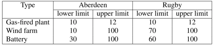
levelR1 = 0. The optimization constraint are shown in Table 1. We setYmin = 10MW,Ymax

= 12 MW,SmaxandRmaxto be 100 MW for both cities. SetSminas10and70MW,Rminas30

and60MW, respectively, for Aberdeen and Rugby. Due to the problem set-up and feasibility constraints we impose in (3), the values for lower limit are set on the boundary between the feasible and infeasible domains.

Type Aberdeen Rugby

lower limit upper limit lower limit upper limit

Gas-fired plant 10 12 10 12

Wind farm 10 100 70 100

Battery 30 100 60 100

Table 1 Lower and upper capacity limit in MW for each plant

The typical lifetime for a wind turbine is about 20 years, for gas-fired plant 30 years and for the battery 15 years. We assume investment cost can be spread over the lifetime of a plant. Both investment cost and annual O/M cost are usually stated as the cost per MW in the literature, which are shown in Table 2. We assume the cost functions are linear in our numerical examples. There is a fixed operation cost for the battery and a variable cost for charging and discharging. Of course, if more detailed cost information is available, it may help to work out more appropriate forms for the cost functions, and this can be easily adopted in our model.

Type Investment cost (£/MW) O/M cost (£/MW)

Gas-fired plant 17484 20981

Wind turbine 37000 24000

Battery 51260 6015 (fixed), 1.05 (variable)

We consider the following linear cost functions,

Ig(Yg) = aYg, Is(Sw) = bSw, Is(Rs) = cRs,

Mg(Yt) =xYt, Mw(Wt) = yWt, Ms(Rt) =z1+z2Rt.

wherea,b, c,x, y,z1 andz2 are the corresponding cost coefficients shown in Table 2. That is,

a = 17484, b = 37000, c = 51260, x = 2.4, y = 2.7, z1 = 0.69andz2 = 0.00012. Note that

a, b, care the annual values, whereas,x, y, z1, z2are the per-time-period costs.

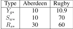
Let(Y_g∗, S_w∗, R∗_s)denote the vector of optimal solutions, measured in MW.

Type Aberdeen Rugby Yg∗ 10 10.9

Sw∗ 10 70

Rs∗ 30 60

Table 3 Optimal capacities for energy storage and generators

With the above choice of parameter values, we implement the optimization problem in MATLAB, which returns optimal capacities (Y_g∗, S_w∗, R∗_s) = (10, 10, 30) with a total cost of £2.63 million for Aberdeen for the year 2012. In other words, optimality requires a 10 MW gas-fired plant and a wind farm capacity of 10 MW (e.g., five turbines with a capacity of 2 MW each). In order to store the surplus generated by the wind turbine(s) during the 8736 time periods, we need a battery that has a usable capacity of 30 MW (or several batteries that add up to a total usable capacity of 30 MW). If the maximum usable capacity of a battery is only 80% of its nominal capacity, then it requires a nominal capacity of 37.5 MW. On the other hand, the optimal capacities are(Y_g∗, S_w∗, R∗_s)= (10.9, 70, 60) for Rugby. The total cost over the year 2012 is estimated to be£6.36 million for Rugby, which is higher than for Aberdeen. We note that the optimal capacities of gas-fired plant are similar for the two cities, while the capacities of wind turbine and battery are much bigger for Rugby. This is expected as wind is much stronger in Aberdeen. The highest wind speed is up to 35 m/s in Aberdeen, while it is just over 11 m/s in Rugby. Furthermore, wind speed is often above 10 m/s in Aberdeen over the one year period, whereas it is often below 3 m/s in Rugby. For Aberdeen, with the help of a constant supply from the gas-fired plant and consistently high wind speeds, only a small capacity of wind turbine(s) is needed. However, in Rugby wind speed is often below the cut-in speed (3 m/s) and it occasionally goes above 10 m/s. Due to the low wind, a much larger wind turbine is required in order to generate enough power to meet the demand. When the occasional high wind speed coincidentally meets with the low demand, a large turbine can generate a big surplus and this leads to the need of a large battery to store the surplus in preparation for periods with low wind speeds. In practice, the Rugby example may not be realistic as wind farms are often built in windy areas. We include it for comparison purpose only.

4. Modelling of stochasticity

In this section we take into account the uncertainty in wind power generation and electricity consumption. The uncertainty in the availability of wind resource is captured using a Markov chain model. To model the intermittent behaviour of energy demand, we will use the method proposed in [3], which attempts to make long-term forecasting with an hourly accuracy.

4.1. Wind speed

takes into account the time correlation and has been frequently used for the generation of syn-thetic wind speed series [17]. We adopt this approach in our study.

A Markov chain (MC) is a sequence of random variables {Xt}t≥0 such that, for any t =

0,1,2, . . ., the random variable{Xt}can take values from a discrete set of states{i0. . . , iN}

and satisfies the following so-called Markov property for conditional probabilities:

P(Xt+1 =it+1 |Xt=it, Xt−1 =it−1, . . . , X0 =i0) =P(Xt+1 =it+1 |Xt=it).

In other words, the probability of the state at time t+ 1 depends only on the state at timet. DenoteP(Xt+1 =j |Xt=i) =pij for all statesiandj. The transition probability matrix for

a first order MC withsstates can be written as

P = 

  

p1,1 p1,2 · · · p1,s

p2,1 p2,2 · · · p2,s

..

. ... . .. ... ps,1 ps,2 · · · ps,s



  

.

According to the definition, we have

pij ≥0, and s

X

j=1

pij = 1 for all i, j = 1, . . . , s.

The transition probability matrix (TPM) can be constructed by using the following formula [18],

pij =

nij

Ps

j=1nij

,

wherenij represents the number of transitions from state i to state j during one period. The

cumulative probability matrix (CPM)C = [Cik]can be constructed according to [18]:

Cik = k

X

j=1

pij.

A second order MC is defined similarly, i.e., we require

P(Xt+1 =it+1 |Xt=it, Xt−1 =it−1, . . . , X0 =i0)

=P(Xt+1 =it+1 |Xt =it, Xt−1 =it−1).

Denoting

P(Xt+1 =k|Xt=j, Xt−1 =i) =pijk

for all statesi,j andk, we can write a second order transition probability matrix as

˜ P =           

p1,1,1 p1,1,2 · · · p1,1,s

p1,2,1 p1,2,2 · · · p1,2,s

..

. ... . .. ... p1,s,1 p1,s,2 · · · p1,s,s

p2,1,1 p2,1,2 · · · p2,1,s

..

. ... . .. ... ps,s,1 ps,s,2 · · · ps,s,s

Actual data 1st order 2nd order

Mean 10.41 10.33 10.46

Std deviation 6.014 6.31 5.879 Variance 36.16 39.81 34.57

Median 9.252 8.988 9.354

Minimum 0.514 0.500 0.500

Maximum 34.95 35.44 35.28

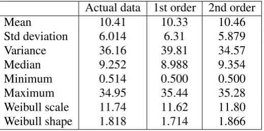
Weibull scale 11.74 11.62 11.80 Weibull shape 1.818 1.714 1.866

Table 4 Descriptive statistics of synthetic and actual data

Similarly, then the CPMC = [Cijk]can be calculated according to [18] as follows:

Cijk = k

X

l=1

pijl.

The MC simulation procedure for synthetic generation of wind speed time-series is accom-plished following the following steps [18]:

1. Define the states of the MC and construct the TPM from the available data. 2. Construct the CPM.

3. Generate uniformly distributed random numbers between 0 and 1. 4. Select an initial statei.

5. Compare the value of the generated random number with the elements ofith row of the CPM. The next state is determined as follows: the value of the random number is greater than the cumulative probability from previous state but no more than that of the following state, sayj. Then the next random number needs to be compared with the elements from thejth row of the CPM.

6. A transition from state i to state j in CPM can be converted into wind speed by Z = Zj−1+Vi(Zj−Zj−1), whereZj−1andZjare the lower and upper boundaries of the state,

Vi is the random number.

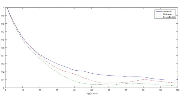
Based on the visual examination of the histogram of the wind speed, the wind speed states have been adopted with an upper and lower limit with a difference of 1 m/s. The upper and lower limit are highly subjective values [19]. In our study, we divide the wind speed data set into 35 states for Aberdeen. For validation of the model, we use a combination of visual evaluation and comparison of statistical properties, which consist of descriptive statistics and Weibull distribution parameters of the probability distribution of the wind speed time-series, as illustrated in Table 4.

Fig. 1. First order MC: Absolute difference between actual and synthetic wind speed

Fig. 2. Second order MC: Absolute difference between actual and synthetic wind speed

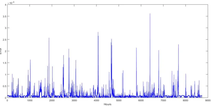
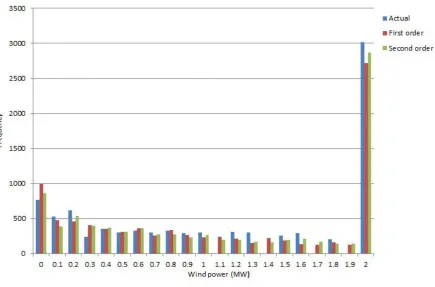
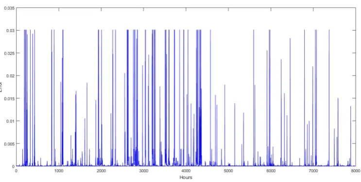
Figure 5 is a bar diagram for the values of energy produced by a 2MW wind turbine for the observed time series and the synthetic time series. The blue bar represents the energy produced from observed, while the red and green bar represent the energy produced from synthetic ones, first and second order respectively. The corresponding hourly errors of wind energy production are shown in Figures 6 and 7.

4.2. Electricity demand

In addition to the intermittency of renewable energy sources as discussed above, the energy demand itself is also intermittent. To model the stochastic behaviour of energy demand, we will use the method proposed in [3]. This method is selected due to its uniqueness in the way that it attempts to make the term forecasting with an hourly accuracy. Traditionally, long-term forecasting is typically performed on a yearly average basis, whereas hourly accuracy is used for short-term prediction. With this method, we are able to forecast the demand load in the long-term with hourly resolution.

Fig. 3. Probability distribution of observed and synthetic wind speed

Fig. 5. Energy produced by a 2MW wind turbine for observed and synthetic wind speed

Fig. 6. First order MC: Absolute difference of wind power generated from actual and synthetic

Fig. 7. Second order MC: Absolute difference of wind power generated from actual and syn-thetic wind speed

and annual energy consumption values from 2005 to 2012. We use half-hourly data at the GB level (national) from the National Grid, which we subsequently aggregate to obtain an hourly-average. The hourly national consumption data is then scaled down to match the value of the annual regional (sub-national) consumption (obtained from the Department of Energy and Climate Change).

The method proposed in [3] consists of three steps. The first step is the modelling of the yearly demand changes, followed by the modelling of the weekly residual variations within a year, and the hourly variations within a week. The model is then constructed by summing these three parts together.

1. Yearly modelling: We use the demand load from 2005 to 2012 and fit a function that approximates the behaviour on the yearly resolution. The yearly resolution can be approx-imated by various functions, such as linear, polynomial or power functions. We consider a linear function with a goodness of fitR2 _{= 0.988.}

Applying a curve fitting algorithm in MATLAB results in the following yearly load model (with 95% accuracy):

f(x) =−3.175x+ 10080, x= 1, . . . ,416,

wherex= 1denotes the first week of 2005 andx= 416the last week of 2012.

2. Weekly residual modelling: We assume that the weekly load model is a combination of the yearly load model and variations on a weekly basis. The weekly variation is obtained by dividing the yearly averaged data, which we call the weekly residual load variations within a year. Since we only have hourly data from 2010 to 2012, we compute the weekly residual data for the period 2010 to 2012 and consider fitting a model. Here we choose to model the weekly residual load by a sum of three sine functions due to the relatively oscillatory behaviour of the available data. The chosen function is considered to be a sum of three terms. We apply a curve fitting algorithm in MATLAB and the resulting functional form (with 95% accuracy) is:

wherexstarts in week 261 from 2005, i.e., week 1 of 2010.

We assume that the weekly residual load variation for 2005 to 2010 can be modelled sim-ilarly to the weekly residual load variation for 2010 to 2012. In other words, we can extend the domain ofg(x)to the period 2005 to 2012. Define the demand load function with weekly resolution,D0(x), as the productf(x)andg(x):

D0(x) = f(x)g(x), forx= 1, . . . ,416.

3. Hourly modelling: We assume that the hourly load model is a combination of the weekly load model and variations on a hourly basis. We observe that the hourly variations within a single week are quite similar throughout the year, and so we assume that the hourly variations within a week can be well represented by the averaged hourly load shape across a week. We denote this shape as the week-to-hour template. Since we have three-years period of hourly data, to avoid the effects of overall increase or decrease within a year, we normalize the template so that the volume under the surface is 1.

We denote the week-to-hour template byT(h, d), wheredrepresents the days of the week and h represents the hours of the day d. To obtain T(h, d), we consider the week-to-hour template as a 24×7 matrix, and apply the 2-D discrete cosine transform (2-D DCT). Next, we pick out the seven entries with the largest magnitude and set all other entries to zero. We then apply the inverse 2-D discrete cosine transform to obtainT(h, d). In this case, only seven coefficients are required to generate the week template data.

We now assume that the model week-to-hour template is representative of the hourly varia-tion within a week. Thus, the demand model with hourly resoluvaria-tion is

D(h, d, x, y) =D0(ˆx)T(h, d)

forh = 1, . . . ,24; d = 1, . . . ,7; x = 1, . . . ,52; andy = 1, . . . ,8; whereD0(ˆx) = f(ˆx)g(ˆx) andxˆ= (52y+x), whileh,d,xandyindicate respectively hours, days, weeks and years from 2005 to 2012.

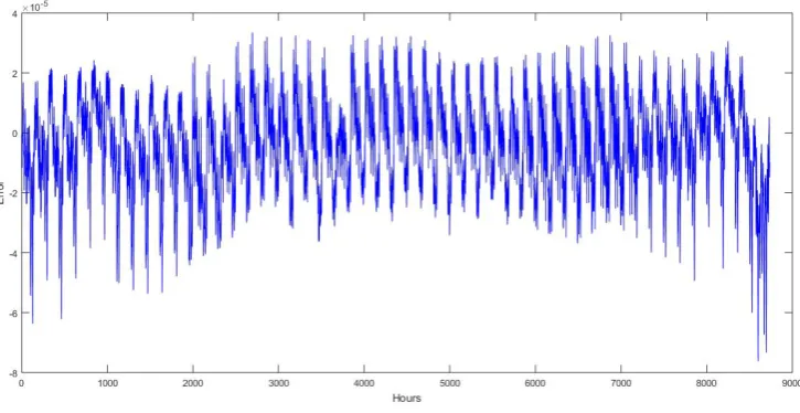
Finally the demand model established in the above three-step procedure is validated by comparing the predicted values with actual values for year 2012, which is shown in Figure 8. The mean absolute percentage error is calculated and displayed in Figures 9 and 10. The former displays the error terms in absolute values, and the latter displays the signed error terms. The blue curve represents the actual consumption level, while the green curve is the predicted consumption level.

From the above analysis, the demand model works quite well. For the calculation of the mean absolute percentage error, we have included the absolute error and the signed error, as it is useful to see when and where the negative values occur within the electricity market. In practice, the negative values are more costly than positive values. The error terms seem to be higher towards the end of the plot (see Figure 9), which may be due to the effect of the Christmas and the New Year period.

Fig. 8. Actual and predicted consumption level of 2012

Fig. 9. Absolute value of error term ofD(h, d, x, y)of 2012

could fit a model with more accuracy and predict more accurately. For the weekly and hourly modelling, it may be helpful to have a longer period of data for further observation and finer tuning. Longer period of data would help increase the goodness of fitR2 in the weekly and hourly fitting. However, we do not expect these changes to be significant.

4.3. Numerical examples

We provide a numerical example as we have done in Section 3.2, but rather than using real data, we use our wind speed simulated with a second order MC model and electricity consumption predicted with the model described above. The other settings will remain the same as described in Section 3.2.

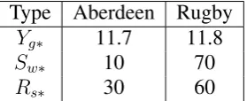
Type Aberdeen Rugby Yg∗ 11.7 11.8

Sw∗ 10 70

Rs∗ 30 60

Table 5 Optimal capacities for energy storage and generators

With the same choice of parameter values, the optimization algorithm returns optimal ca-pacities (Y_g∗, S_w∗, R∗_s) = (11.7,10,30) for Aberdeen and (Y_g∗, S_w∗, R_s∗) = (11.8,70,60) for Rugby. Their corresponding total costs over the year 2012 are£2.73 million and£6.43 million, respectively.

The optimal capacities generated by the stochastic model differ only in the capacity of gas-fired plant. There is respectively a 0.1 million and 0.07 million difference in the total annual cost for Aberdeen and Rugby. Since errors are always present with forecasting or simulating, we expect small changes in the optimal capacities and thus in the total annual cost.

5. Connection to the National Grid

In this section, we relax assumption (a) that we made at the beginning of Section 3 for our basic model by allowing import and export of electricity. That is, if the demand exceeds the sum of the current power generation and the power stored in the battery, then we can import power from the National Grid; and if there is a surplus and our storage device is full, we can export to the National Grid.

5.1. Extended model

We assume that a network connecting to the National Grid already exists, and thus we do not look into the process of how to establish a network. However, we set up the restriction that the National Grid makes up at mostγ% of the demand, and thus this forces our system to generate at least(100−γ)% of the demand all the times, where0≤γ <100.

If we have a deficit at time t, i.e., Dt > Wt+Yt+Rt, then we deplete all the surplus

power in the battery and import the difference from the National Grid. Hence,Rt+1 = 0and

we importGt = Dt−Wt−Yt−Rt > 0. On the other hand, if we have a surplus at timet,

i.e.,Dt < Wt+Yt+Rt, our first priority is to fill up the battery, and then export the remainder

Htto the National Grid. We introduce a degree of flexibility into the system by imposing the

constraint that we only export a certain percentage of the surplus. Consequently, we have the following procedure in the case of surplus: IfRt+1 = Rt+ρR∗(Wt+Yt−Dt) < Rs, then

we export nothing. Otherwise, ifRt+1 > Rs, then we export the amountHt= β(Rt+1−Rs),

of the surplus we will export. For instance, settingβ = 0.1amounts to exporting only 10% of the surplus.

At the same time, we replace the last constraint in (3) with

Gt ≤γDt and Dt≤Wt+Yt+Rt+Gt.

Since connecting to the National Grid may incur other costs (positive or negative) such as costs for distribution or imports, revenue for selling surplus. Accordingly, we add the following term to the objective functional (1):

n

X

t=1

(PeGt−PsHt+ (Ac+AdHt)−PwWt),

wherePeandPsare import and export price of electricity, respectively;Pw is the price paid to

wind farms for energy generation; whileAcandAdare fixed and variable component,

respec-tively, of the distribution charge. The above equation is explained as follows: For each unit of power we import from the National Grid, we pay a price ofPe, thus it generates a cost ofPeGt

in each period. Similarly we obtain a revenue ofPsHtin each period from exporting.

Accord-ing to the National Grid policy, wind farms get paid by the National Grid for power generation regardless whether the power is exported, which leads to a revenue ofPwWt. There are also

charges from the distributors for the power to be distributed while exporting to the National Grid. The charges usually involve a fixed component and a component that varies with the quantity, which lead to the termAc+AdHt.

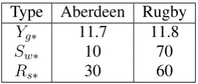
5.2. Numerical examples

We now provide numerical examples in order to make a comparison with the results obtained in Section 4.3. The setting remains the same withPeandPsobtained from Elexon. The price

paid for generation is obtained from Ofgem’s website,Pw = 3.41p/kWh. The distribution cost

differs from region to region, which is usually made up of a fixed component and a component that varies with quantity. For Aberdeen, the daily fixed componentAc = 5.45p/kW, whereas

the variable costAd is 1.22 p/kW during peak period, and 0.17 p/kW during off-peak period.

For Rugby, there is no fixed cost,Ac= 0. The variable costAdis 2.13 p/kW during peak time

and 0.43 p/kW during off-peak time. In our study, we consider peak time as 7am–7pm, and set γ = 0.1andβ = 0.1.

Type Aberdeen Rugby Yg∗ 11.7 11.8

Sw∗ 10 70

Rs∗ 30 60

Table 6 Optimal capacities for energy storage and generators

Fig. 11. Amount to be exported to the National Grid at each period for Aberdeen and Rugby

with connection to the National Grid, the surplus from wind that would otherwise be dumped can be sold to the National Grid to make some revenue after filling up the battery.

Figure 11 shows the amount exported to the National Grid, where blue bars represent the export from Aberdeen and red bars from Rugby. As shown in category0, Rugby does not have any export for over half of the periods over the one-year period. However, occasionally it can export more than 1 MW per time period. Whereas, Aberdeen is more consistent, exporting for over 80% of the time periods. Based on the amount exported, the total cost has decreased by 0.23 million and 0.13 million for Aberdeen and Rugby, respectively.

6. Conclusions

In this study, we have investigated the joint optimization of renewable generation and energy storage by formulating the problem in a cost minimization framework. We want to determine optimal capacities for the generator and storage that minimize the associated total cost, provid-ing demand is met all the time. The problem is first formulated as a deterministic model and then extended to increase its flexibility. We have also studied how the system can operate more efficiently and economically. As future work, we will include the effects of other storage tech-nologies by studying their characteristics and modifying the corresponding cost functionals.

Acknowledgments

Disclaimer

Monica Giulietti is a member of the panel of technical experts for the delivery of the Electricity Market Reform. However she has carried out this work in her academic capacity only and has relied exclusively on publicly available data and information. The views expressed in this work do not reflect those of the other panel members nor those of the UK Department of Energy and Climate Change.

7. References

[1] IEA. International Energy Agency: World energy outlook. International Energy Agency

Publications, 2011.

[2] A. Rhodes. Smart grids: Commercial opportunities and challenges for the uk. future and emerging opportunities manager, energy generation and supply. Technical Report,

Knowledge Transfer Network, 2010.

[3] ¨U. Filik, ¨O. Gerek, and M. Kurban. A novel modeling approach for hourly forecasting of long-term electric energy demand. Energy Conversion and Management, 52(1):199–211, 2011.

[4] J. Garcia-Gonzalez, R. de la Muela, L. Santos, and A. Gonzalez. Stochastic joint opti-mization of wind generation and pumped-storage units in an electricity market. Power

Systems, IEEE Transactions, 23(2):460–468, 2008.

[5] E. Fertig and J. Apt. Economics of compressed air energy storage to integrate wind power: A case study in ercot. Energy Policy, 39:2330–2342, 2011.

[6] C. Abbey and G. Joos. A stochastic optimization approach to rating of energy storage systems in wind-diesel isolated grids. Power Systems, IEEE Transactions, 24(1):418– 426, 2009.

[7] P. Yang and A. Nehorai. Joint optimization of hybrid energy storage and generation ca-pacity with renewable energy. IEEE Transactions on Smart Grid, 5(4):1566–1574, 2014.

[8] R. Abbassi and S. Chebbi. Energy management strategy for a grid-connected wind-solar hybrid system with battery storage: Policy for optimizing conventional energy generation.

International Review of Electrical Engineering, 7(2):3979–3990, 2012.

[9] S. Abbassi, R. Salem, M. Hammami, and S. Chebbi. Analysis of renewable energy power systems: Reliability and flexibility during unbalanced network fault, handbook of research on advanced intelligent control engineering and automation. IGI Global, pages 651–686, 2015.

[10] D. Villanueva, J.L. Pazos, and A. Feijoo. Probabilistic load flow including wind power generation. Power Systems, IEEE Transactions, 26(3), 2011.

[11] J.H. Kim and W.B. Powell. Optimal energy commitments with storage and intermittent supply. Journal of Operations Research, 59:1526–5463, 2011.

[12] IEA. International Energy Agency: Energy technology systems analysis programme.

Energy Technology Network, 2010.

[14] R. Carnegie, D. Gotham, D. Nderitu, and P. Preckel. Utility scale energy storage systems. 2013.

[15] ARUP. Five minute guide - electricity storage technologies. ARUP Group Limited, 2013.

[16] A. Akhil, G. Huff, and A. Currier. Sandia report.Electric Power Research Institute, 2013.

[17] A. Carpinone, R. Langella, A. Testa, and M. Giorgio. Very short-term probabilistic wind power forecasting based on markov chain models. Probabilistic Methods Applied to

Power Systems, IEEE 11th International Conference, pages 107–112, 2010.

[18] S. Karatepe and K. Corscadden. Wind speed estimation: Incorporating seasonal data using markov chain models. ISRN Renewable Energy, 2013.