Analysis of coronal rain observed by IRIS, HINODE/SOT and SDO/AIA : transverse oscillations, kinematics and thermal evolution

warwick.ac.uk/lib-publications

Original citation:

Kohutova, Petra and Verwichte, E. (Erwin). (2016) Analysis of coronal rain observed by IRIS,

HINODE/SOT and SDO/AIA : transverse oscillations, kinematics and thermal evolution. The

Astrophysical Journal, 827 (1). 39.

Permanent WRAP URL:

http://wrap.warwick.ac.uk/79759

Copyright and reuse:

The Warwick Research Archive Portal (WRAP) makes this work by researchers of the

University of Warwick available open access under the following conditions. Copyright ©

and all moral rights to the version of the paper presented here belong to the individual

author(s) and/or other copyright owners. To the extent reasonable and practicable the

material made available in WRAP has been checked for eligibility before being made

available.

Copies of full items can be used for personal research or study, educational, or not-for-profit

purposes without prior permission or charge. Provided that the authors, title and full

bibliographic details are credited, a hyperlink and/or URL is given for the original metadata

page and the content is not changed in any way.

Publisher’s statement:

http://iopscience.iop.org/journal/0004-637X

A note on versions:

The version presented here may differ from the published version or, version of record, if

you wish to cite this item you are advised to consult the publisher’s version. Please see the

‘permanent WRAP URL’ above for details on accessing the published version and note that

access may require a subscription.

Preprint typeset using LA_{TEX style emulateapj v. 01/23/15}

ANALYSIS OF CORONAL RAIN OBSERVED BY IRIS, HINODE/SOT AND SDO/AIA: TRANSVERSE OSCILLATIONS, KINEMATICS AND THERMAL EVOLUTION

P. Kohutova & E. Verwichte

Centre for Fusion, Space and Astrophysics, Department of Physics, University of Warwick, Coventry CV4 7AL, UK; [email protected]

Draft version June 6, 2016

ABSTRACT

Coronal rain composed of cool plasma condensations falling from coronal heights along magnetic field lines is a phenomenon occurring mainly in active region coronal loops. Recent high resolution observations have shown that coronal rain is much more common than previously thought, suggesting its important role in the chromosphere-corona mass cycle. We present the analysis of MHD oscillations and kinematics of the coronal rain observed in chromospheric and transition region lines by IRIS, Hinode/SOT and SDO/AIA. Two different regimes of transverse oscillations traced by the rain are detected: small-scale persistent oscillations driven by a continuously operating process and localised large-scale oscillations excited by a transient mechanism. The plasma condensations are found to move with speeds ranging from few km s−1_{up to 180 km s}−1 _{and with accelerations largely}

below the free fall rate, with the likely reasons being pressure effects and the ponderomotive force resulting from the loop oscillations. The observed evolution of the emission in individual SDO/AIA bandpasses is found to exhibit clear signatures of a gradual cooling of the plasma at the loop top. We determine the temperature evolution of the coronal loop plasma using regularised inversion to recover the differential emission measure (DEM) and by forward modelling the emission intensities in the SDO/AIA bandpasses using a two-component synthetic DEM model. The inferred evolution of the temperature and density of the plasma near the apex is consistent with the limit cycle model and suggests the loop is going through a sequence of periodically repeating heating-condensation cycles.

Keywords: magnetohydrodynamics (MHD) - Sun: corona - Sun: magnetic fields - Sun: oscillations

1. INTRODUCTION

High resolution observations from recent solar missions have unveiled a dynamic nature of the solar corona and enabled us to study the coronal activity in unprecedented detail (Scullion et al. 2014). The basic structure of the corona is formed by coronal loops; magnetic flux tubes confining the coronal plasma threading through the solar surface. They are highly dynamic and subject to a range of matter and energy transport processes. One of such processes is the coronal rain, consisting of cool plasma condensations falling from coronal heights to the solar surface guided by the magnetic field lines (Schrijver 2001; De Groof et al. 2004).

Despite being first observed more than 40 years ago (Kawaguchi 1970; Leroy 1972), coronal rain has not re-ceived much attention up until recent years. This was partially due to the lack of instruments with resolution sufficient for detailed observations. Coronal rain was also believed to be a relatively rare phenomenon oc-curring only sporadically in active regions on the time scales of days (Schrijver 2001). Recent work has how-ever shown that the coronal rain is in fact much more common that previously thought, typically occurring on the time scales of hours (Antolin et al. 2010; Antolin & Rouppe van der Voort 2012). This short period of a typical heating-condensation cycle together with the fact that a significant fraction of coronal loops are out of hy-drostatic equilibrium constantly undergoing heating and cooling phases (Aschwanden et al. 2001) and hence prone for the condensation to occur suggest that coronal rain may have an important role in the chromosphere-corona

mass cycle (Marsch et al. 2008; Berger et al. 2011; McIn-tosh et al. 2012).

The formation of coronal rain is believed to be linked to rapid cooling of thermally unstable coronal loops (M¨uller et al. 2003, 2004, 2005). Concentrated footpoint heat-ing leads to uneven temperature profile along the loop length. Chromospheric evaporation and direct injection of plasma into the corona result in high densities near the top of the loop. In the case of insufficient thermal con-duction, the radiation losses near the loop top overcome the heating input resulting in an onset of a thermally un-stable regime. A perturbation to the loop such as shock wave can then trigger catastrophic cooling leading to the formation of condensations which subsequently fall down towards the solar surface along the magnetic field lines within the coronal loop. This process continues until the heating and cooling regain equilibrium and pressure bal-ance is restored.

both pointing towards continuous heating and cooling scenario. The cooling sequence has also been observed in loops exhibiting coronal rain (Antolin et al. 2015b). Such peak intensity variations with time and wavelength are therefore likely to be a signature of the thermal instabil-ity in the loops. On larger scale, the occurrence interval of the thermal instability onset leading to formation of the coronal rain in a loop with footpoint-concentrated heating is estimated to be on a time scale of several hours (Antolin & Rouppe van der Voort 2012). Simi-lar long term periodic EUV pulsations with periods of several hours were observed in warm active region coro-nal loops (Auch`ere et al. 2014; Froment et al. 2015), as well as in prominences (Foullon et al. 2004, 2009).

Coronal rain is usually observed in emission in cool chromospheric lines of both neutral (Hα, Lyα) and ionosed atoms (Ca II, He II); or in absorption in EUV (Schrijver 2001). The temperatures of the rain plasma range from transition region (∼ 105 _{K) to}

chromospheric(∼104K). Coronal rain has been detected in the 304 ˚A channel of SDO/AIA (Kamio et al. 2011) and SOHO/EIT (De Groof et al. 2004, 2005), in the 1600 ˚

A channel of TRACE (Schrijver 2001), in Ca II H line using Hinode/SOT (Antolin et al. 2010; Antolin & Ver-wichte 2011), in the Hαby the SST/CRISP (Antolin & Rouppe van der Voort 2012) and in IRIS FUV and NUV channels (Kleint et al. 2014). Material resembling coro-nal rain has recently been observed in photospheric wave-lengths by SDO/HMI (Mart´ınez Oliveros et al. 2014). Despite best resolved coronal rain being usually observed off-limb, some on-disk coronal rain events have also been observed (e.g. Antolin et al. 2012; Antolin & Rouppe van der Voort 2012).

The thermal instability onset and the process of forma-tion and evoluforma-tion of the coronal rain have been subject to a number of numerical studies. Such studies were ini-tially restricted to simplified 1-dimensional cases. One of the first attempts to model the formation of the conden-sation region and its subsequent evolution was done by M¨uller et al. (2003, 2004, 2005), indicating that a loop with exponential heating function localised at the foot-points develops a thermal instability followed by catas-trophic cooling. This basic model was further expanded by Antolin et al. (2010) by accounting for variable loop cross-section, impulsive nature of heating and Alfv´en wave dissipation near the footpoints. More recently, the formation process of coronal rain condensations and their evolution was studied by 2.5D MHD simulations (Fang et al. 2013, 2015). The evolution of condensations for the case of fully ionized plasma was further analysed by Oliver et al. (2014), emphasising the role of the pressure effects on the coronal rain dynamics.

The small size of coronal rain blobs makes it suit-able for tracing the strength and structure of the coronal magnetic field (Antolin & Rouppe van der Voort 2012). The degree to which the rain follows the direction of the magnetic field however depends on the strength of the coupling between recombined atoms created during the condensation phase and the local ion population. In the case of the strong coupling, any disturbance of the magnetic field in the loop will be reflected in the mo-tion of the rain blobs. A number of observamo-tions have shown presence of transverse MHD waves in the

coro-nal loops (Aschwanden et al. 1999; Nakariakov et al. 1999). These are commonly interpreted as a fast kink MHD mode (Edwin & Roberts 1983; Nakariakov & Ver-wichte 2005; Van Doorsselaere et al. 2008; Goossens et al. 2009). Multiple regimes of such oscillations have been detected, ranging from periods on the order of seconds (e.g. Williams et al. 2001) to hours (e.g. Hershaw et al. 2011). Both standing (Nakariakov et al. 1999; White & Verwichte 2012) and travelling regimes (Williams et al. 2001; Tomczyk et al. 2007; McIntosh et al. 2011) of the kink oscillations are observed. They can be excited by a flare or other energetic event and subject to rapid at-tenuation (White et al. 2012; White & Verwichte 2012; Nistic`o et al. 2013), possibly caused by resonant absorp-tion (Hollweg & Yang 1988; Ruderman & Roberts 2002; Goossens et al. 2002, 2010; Okamoto et al. 2015; An-tolin et al. 2015a); or persistent and decay-less, driven by a continuous process (Wang et al. 2012; Nistic`o et al. 2013; Anfinogentov et al. 2013). Coronal rain occurring in a loop oscillating transversely will also be subject to transverse oscillatory motion. Such MHD oscillations in coronal rain were first detected by Antolin & Verwichte (2011). In the case of a non-negligible inertia of the coro-nal rain blobs, the rain itself can have an effect on the loop oscillations.

MHD oscillations in coronal rain can therefore (1) af-fect dynamics of the coronal rain through a ponderomo-tive force exerted on the falling blobs, (2) help to quan-tify the effect of the plasma condensations on the coronal loop and (3) have coronal seismological potential and be a source of information about coronal loop properties and the magnetic field structure in the loop. This highlights the importance of addressing the interplay between the coronal rain and MHD waves in order to better under-stand the coronal loop structure, evolution and energy transport mechanisms.

The paper is organized as follows: Section 2 covers the details of IRIS, Hinode/SOT and SDO/AIA observations used for analysis and the methods used for data process-ing. Section 3 focuses on analysis of MHD oscillations detected in the coronal rain. In section 4 we investi-gate the kinematics of individual coronal rain blobs and present statistics of blob velocities and accelerations. In section 5 we analyse the evidence for the thermal evo-lution of the loop plasma and the heating-condensation cycle of the coronal loop responsible for the coronal rain formation. Section 6 contains detailed discussion of the analysis outcomes and their implications. The work is summarised in section 7.

[−98400,−19600] in solar heliocentric coordinates. We further used Hinode level 0 Ca II H data centered at [−99300,−20500] in solar heliocentric coordinates, with the exposure time of 1.229 s and 12 s cadence taken be-tween 8:20 and 9:37 UT. Using the AIA Cutout Service (http://www.lmsal.com/get aia data/) we retrieved the required subframes of level 1.5 SDO/AIA data with 12 s cadence that were normalised by the exposure time.

IRIS level 2 and SDO/AIA level 1.5 data used in this work already include geometric correction, dark correc-tion and flat-fielding. The dark current correccorrec-tion and the flat-fielding of the Hinode level 0 data was carried out using the fg prep Solarsoft routine. The data fur-ther required additional pre-processing in order to be suitable for the coronal rain analysis, in particular noise reduction, edge enhancement and removal of trends in brightness variation across the data cube. Two dimen-sional Mexican hat wavelet transform filtering was used to achieve this by enhancing the features in the image with sizes close to the characteristic scale of the wavelet (Witkin 1983; White & Verwichte 2012).

We focus on a coronal loop outlined in Figure 1 show-ing IRIS Si IV SJI data. The loop is visible durshow-ing the whole observing sequence; the coronal rain occurring in the loop can be observed for about an hour. The stud-ied loop does not cross the spectrograph slit; no spectral information is therefore available and the analysis is re-stricted to the imaging data. The coronal rain is visible in IRIS FUV and NUV, Hinode Ca II H and SDO/AIA 304 ˚A bandpasses suggesting a multithermal nature of the phenomenon. The individual plasma condensations are best discernible in the Si IV line (1400 ˚A), which was therefore chosen for analysis.

The studied loop exhibits significant amount of coro-nal rain downflows as well as upflowing material. Most of the upward flow of the plasma occurs in the remote leg while the condensations are falling down preferentially along the loop leg closer to the observer. This asymme-try is likely caused by a background siphon flow due to a pressure difference between the footpoints. Such back-ground flow can move the region where the thermal in-stability and subsequent condensation occurs to the side away from the apex resulting in coronal rain falling along one leg only.

The view of the observed event is limited to a single vantage point, we can therefore only make approximate estimates about the loop geometry. The loop plane ap-pears approximately perpendicular to the solar surface. The positions of the axis of the loop, loop apex and foot points were determined from a series of multiple SJI time frames superimposed on each other to highlight the flows of the material in the loop. Multiple strands of plasma tracing the loop’s magnetic field lines are observed, the loop therefore appears to have considerable thickness. The radius of the loop was estimated to be 40.9 Mm using the distance from the apex to the loop baseline connecting the two footpoints. Assuming the loop has a semitoroidal shape, the estimate of the loop radius and the observed projected distance between the footpoints of 12.8 Mm was used to estimate the angle between the loop plane and the line-of-sight to be 9◦.

The plasma condensations falling along the coronal loop are found to have considerable thickness of about

0.5 Mm, often grouping into strands. The individual strands clearly exhibit transverse oscillations which are best visible near the loop apex. The strands were ob-served to separate and merge again multiple times, thus complicating the tracking of the individual plasma blobs. The most pronounced elongation of the plasma blobs into strands occurs in the lower half of the loop. Individual strands were observed to converge as approaching the loop footpoints.

Longer duration AIA 304 ˚A dataset covering two 12 hour windows before and after the coronal rain event observed by IRIS and Hinode shows that it is a part of a sequence of successive coronal rain events occurring in the same coronal loop. A total of 4 events were detected on the day of observation. Other events were however much less clear due to multiple short-lived rainy loops appearing in the foreground, detailed analysis of the full 24 hour AIA dataset has therefore not been carried out.

3. OSCILLATIONS

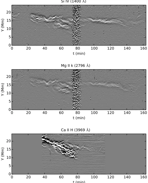
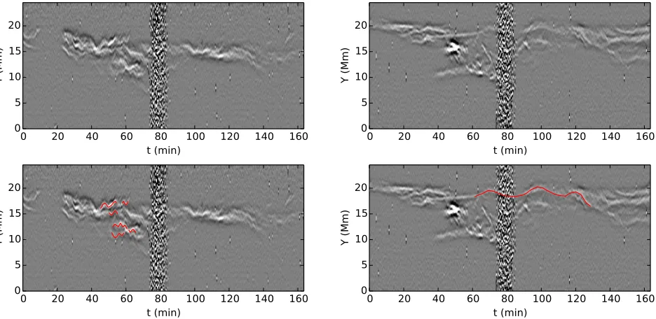
In order to detect any transverse oscillations of the structure, we set up 10 slits perpendicular to the loop axis (Figure 1). A cut through data was then taken along each slit and the data was superimposed over 30 pixels in longitudinal direction to detect oscillations of small blobs as well as of longer strands. The longitudinal superpo-sition length was chosen as being long enough to detect short strand oscillations and short enough to capture any behaviour dependent on the longitudinal distance. The cuts at each time step were then stacked to create time distance plots, each corresponding to different position along the loop. The time distance plots created using aligned IRIS Si IV, Mg II k and Hinode Ca II H data show large degree of similarity with the majority of strand-like structures being identifiable in all three wavelengths (Figure 2). This co-spatial emission suggests multither-mal nature of the coronal rain plasma. Time distance plots created using IRIS Si IV observations correspond-ing to two slits, one at the loop apex and another 22 Mm above the footpoint are shown in Figure 3. Mul-tiple transverse oscillations are visible along the whole loop length. The contamination lasting from 75 min to 85 min in the IRIS observational sequence is caused by a surge of particles due to the spacecraft passing through the South Atlantic Anomaly.

Due to the large number of strands present at the same longitudinal distance, traditionally used automated strand detection methods based on fitting a Gaussian to the image intensity profile at each time step (Verwichte et al. 2009, 2010) proved unsuitable. The strand centre coordinates were therefore extracted manually from the time-distance plot for each slit to avoid errors that an automated procedure might introduce due to the nature of the intensity profiles. The strand centre displacement time series for each oscillation was then extracted and fit-ted with functionξ(t) =ξ0sin(ωt+ Φ) using

Levenberg-Marquardt algorithm in order to determine oscillation parameters. 150 oscillations were observed in total. The standard deviations on the best fit parameters for the individual oscillations were found to be 7%, 3% and 40% for the amplitude, period and phase respectively.

−1000 −500 0 500 1000 X-position [arcsec]

−1000 −500 0 500 1000

Y-p

osi

tio

n [

arc

se

c]

SDO AIA 171.0 Angstrom 2014-08-25 08:52:59

10 20 30 40 50 60 70 80 90

X (Mm) 10

20 30 40 50 60 70 80

Y (

Mm

)

Figure 1. Left: Complete field of view of the IRIS Si IV observation used for analysis with the axis of the studied loop outlined. The cuts for the time-distance plots were taken along 10 slits perpendicular to the loop axis. Right: Position of IRIS field of view in the full-disk image as seen by SDO/AIA.

0 20 40 60 80 100 120 140 160

t (min) 0

5 10 15 20

Y (

Mm

)

Si IV (1400 Å)

0 20 40 60 80 100 120 140 160

t (min) 0

5 10 15 20

Y (

Mm

)

Mg II k (2796 Å)

0 20 40 60 80 100 120 140 160

t (min) 0

5 10 15 20

Y (

Mm

)

Ca II H (3969 Å)

Figure 2. Time-distance plots corresponding to slit near the apex in IRIS Si IV (top), Mg II k (centre) and Hinode Ca II H line (bot-tom). Hinode data was interpolated to match IRIS time resolution and time range. Co-spatiality of the plasma emission suggest a multithermal nature of the coronal rain. Note somewhat different features at t = 40-50 min captured by Hinode only.

loop length but being most prominent in the upper part of the loop; and long period oscillations visible only in the lower half of the loop. We repeat above analysis using

SDO/AIA observations in 171 ˚A. Due to the 1.500 reso-lution of SDO/AIA, only long period oscillation regime can be observed. Figure 4 shows the variation of the os-cillation amplitude with the longitudinal distance of the corresponding slit from the loop apex corrected for the projection effects. There is no clear trend in the ampli-tude variation; however, the plot shows the distribution of the two populations of oscillations.

The amplitudes of the short period oscillations were found to mostly lie within a range 0.2 - 0.4 Mm. No prominent damping of the individual oscillations was ob-served, although one should note that since only few peri-ods of the individual oscillating strands can be observed, any gradual damping is likely to remain undetected. The mean period of the short period oscillations was found to be 3.4 min. The scatter of the periods of the individual oscillations around the mean value is likely to be a result of the uncertainty on the period measurements. If, de-spite the measurement errors, this scatter was real, vary-ing periods of the oscillations detected in different posi-tions within the loop would suggest large variaposi-tions in the properties of the coronal loop plasma. However, due to the fact that a certain level of a collective behaviour of individual strands has been observed, we consider this scenario unlikely. A change of the mean oscillation period with time would in turn imply a presence of a non-linear driving process.

0

20

40

60

80 100 120 140 160

t (min)

0

5

10

15

20

Y (

Mm

)

0

20

40

60

80 100 120 140 160

t (min)

0

5

10

15

20

Y (

Mm

)

0

20

40

60

80 100 120 140 160

t (min)

0

5

10

15

20

Y (

Mm

)

0

20

40

60

80 100 120 140 160

t (min)

0

5

10

15

20

Y (

Mm

)

Figure 3. Time-distance plots corresponding to slits near the apex (left) and 22 Mm above the footpoint (right). We repeat both plots with the oscillation patterns highlighted (bottom). Small scale oscillations are present in both plots. A prominent large scale oscillating structure is visible only in the lower part of the loop. The particle contamination occurring during 75-85 min is due to the spacecraft passing through the South Atlantic Anomaly.

0 10 20 30 40 50 60

Slit distance along the loop (Mm) 0.0

0.2 0.4 0.6 0.8 1.0 1.2 1.4

Am

pli

tud

e (

Mm

)

IRIS 1400

AIA 171

Figure 4. Variation of oscillation amplitude with the longitudinal distance of each slit from the loop apex corrected for projection effects.

due to the thickness of the individual strands.

The presence of synchronous oscillations of nearby strands together with the standing wave assumption points towards a number of possible scenarios for the nature of the wave in the coronal loop responsible for the observed oscillation patterns; one such possibility is a global kink mode affecting the coronal loop as a whole. Alternatively, multiple kink modes present in the loop af-fecting each strand separately could cause in-phase trans-verse oscillating behaviour if triggered by a common source. Short period oscillations traced by the coronal rain with similar characteristics as described above were reported previously (Antolin & Verwichte 2011).

Amplitudes of the long period oscillations observed in IRIS 1400 ˚A passband are of the order of 1 Mm. When observing the cool coronal rain plasma emitting at the chromospheric wavelengths they appear to be most pro-nounced in the lower part of the loop and fading higher

up. At a distance of 37 Mm from the apex they can-not be observed at all. This is due to the cool plasma being more sparse in the upper part of the loop dur-ing the latter half of the observational sequence, which complicates tracking of long period oscillatory patterns. In the hot coronal wavelengths the long period oscilla-tions are observable along the whole loop length, having similar periods as in IRIS observations but lower am-plitudes (Figure 4). This amplitude discrepancy can be attributed to limited resolution of SDO/AIA, with the typical peak to peak amplitude of this oscillation regime being 3 pixels. At such short scales, the standard devi-ation of best-fit oscilldevi-ation parameters estimated from a sample oscillation pattern might be an underestimate of the true uncertainty. The mean period of this oscillation regime is 17.4 min, i.e. much longer than typical period of the fundamental standing mode of the kink oscillation expected for a loop with comparable length. This sug-gests that the oscillatory pattern is a manifestation of a propagating rather than standing wave. In the propagat-ing wave scenario the expected phase shift for such long period oscillations would be too small to be observed in the dataset with this duration.

4. KINEMATICS

The kinematics of the plasma condensations was anal-ysed by tracking the individual blobs along their paths over the period during which they could be observed in the given bandpass. The individual plasma blobs were best discernible in the data taken in the IRIS Si IV filter, which was therefore chosen for kinematics analysis. Not all plasma blobs were observable during their entire mo-tion from loop apex all the way to the footpoints; this is likely due to change in emission in the SI IV line following a temperature change.

0 10 20 30

Projected distance (Mm)

0

20

40

60

80

100

120

140

160

Tim

e (

mi

n)

0 10 20 30

Projected distance (Mm)

0

20

40

60

80

100

120

140

160

Tim

e (

mi

n)

0 10 20 30 40

Projected distance (Mm)

0

20

40

60

80

100

120

140

160

Tim

e (

mi

n)

Figure 5. Time-distance plots extracted along 3 different paths followed by condensations. The horizontal axis corresponds to the projected distance along the path. The bright traces correspond to trajectories of individual blobs. In the rightmost plot, a number of blobs can be observed to oscillate around the loop top before falling down to the solar surface. The faint features stationary in the longitudinal direction are caused by background loops intersecting the axis of the studied coronal loop.

plot was extracted. Three such time-distance plots are shown in Figure 5. The bright traces correspond to the trajectories of the individual condensations. A total of 115 plasma blobs were tracked, out of which 18 were part of the upflowing material and the remaining 97 blobs were falling condensations. In the subsequent analysis we focused on the coronal rain blobs. We extracted their trajectories and corrected them for projection effects by calculating the real distance travelled along the loop cor-responding to the observed distance of the blob from the apex (assuming 9◦loop plane angle and semicircular loop axis). For each blob an initial and final velocity was determined, enabling us to deduce mean acceleration of each blob.

The initial and final velocities and mean accelerations of the coronal rain blobs are shown in Figure 6. The distribution of velocities is broad ranging from small velocities of only few km s−1 _{to large velocities over}

150 km s−1_{, with the mean velocity being 45 km s}−1_.

The variation of the observed velocity with height is shown in Figure 7. The observed velocities of the in-dividual blobs are largely below free-fall values, shown by the solid line. The distribution of blob accelera-tions is on the other hand much narrower and is clus-tered around the mean acceleration of 95 m s−2_{. The}

average effective gravity along an ellipse is given by

hgef fi= 2/π

Rπ/2

0 gcosθ(s)dswheresis the coordinate

along the ellipse and θis the angle between the tangent to the path and the vertical. If assuming a semicircular loop axis, the average effective gravity along the loop is 174 m s−2. The measured average acceleration is there-fore significantly lower than what would be expected for a free-fall motion. Such sub-ballistic fall rates of coronal rain condensations were reported previously (Schrijver 2001; De Groof et al. 2004; Antolin et al. 2010; Antolin & Verwichte 2011; Antolin & Rouppe van der Voort 2012). Complete velocity and acceleration profiles of individual blobs also show multiple acceleration and deceleration phases as opposed to purely accelerated motion expected if the blobs would be moving solely under the influence of gravity.

5. HEATING-CONDENSATION CYCLE

0 20 40 60 80 100 120 140 160 180_{Velocity (km/s)} 0

5 10 15 20 25 30 35

N

−400 −200 00 _{Acceleration (m/s)}200 400 600 800 1000 1200 2

4 6 8 10

N

Figure 6. Left: the distribution of blob initial (red) and final velocities (black). Right: The distribution of mean blob accelerations. The dashed lines correspond to the average values of 45 km s−1_{and 95 m s}−2 _{for velocities and accelerations respectively.}

5 10 15 20 25

Height (Mm) 0

50 100 150 200

Ve

loc

ity

(k

m/

s)

Figure 7. Dependence of blob velocity on the height above the so-lar surface. The velocity dependence expected for a free fall motion is shown by the solid line and the velocity dependence expected for a motion with the mean observed acceleration of 95 m s−2_{is shown}

by the dashed line.

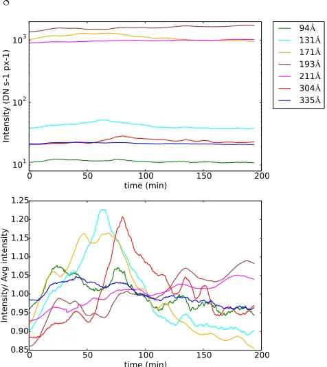
emission in 94 ˚A, 131 ˚A, 171 ˚A, 193 ˚A, 211 ˚A, 304 ˚A and 335 ˚A. The emission first peaks in 94 ˚A, followed by peaks in 335 ˚A, 171 ˚A, 131 ˚A and 304 ˚A, i.e. in pro-gressively cooler bandpasses. It should be however noted that low intensities measured in 94 ˚A and 335 ˚A suggest that uncertainties in these light curves are large, thus reducing their reliability. In addition, the lack of single well-defined peak in the instrumental response functions of the 94 ˚A and 335 ˚A channels (Boerner et al. 2011) makes it non-trivial to infer a cooling sequence from the light curves in these two channels. The emission in 193 ˚

A and 211 ˚A is on the other hand observed to be steadily increasing, with a number of secondary peaks. The se-quence of prominent peaks in 171 ˚A, 131 ˚A and 304 ˚A channels therefore clearly suggests a gradual cooling of the plasma at the loop top, while the emission in 94 ˚A, 335 ˚A, 193 ˚A and 211 ˚A channels does not provide addi-tional evidence of cooling.

We further estimate the temperature distribution of the emission of the loop plasma integrated along the line of sight as a function of time. This can be quantified by the differential emission measure (DEM)ξ(T) defined as

0 20 40 60 80 100 120

X (arcsec) 0

20 40 60 80 100 120

Y

(a

rc

se

c)

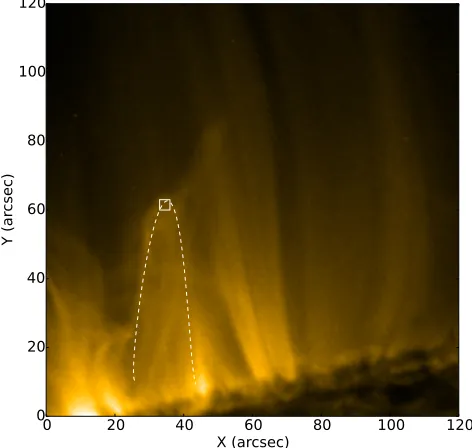
Figure 8. SDO/AIA 171 ˚A view of the studied coronal loop. The marked region at the loop top used to obtain the evolution of the intensity of the emission.

ξ=n2_edz

dT (1)

whereneis the electron density,zis the distance along the line of sight andT is the temperature. The observed intensities are a result of a convolution of the DEM with the instrumental response functions:

Fi=

Z

ξ(T)Ri(T)dT (2)

whereFiis the intensity measured in theith bandpass and Ri is the instrumental response function of the ith filter dependent on the temperature. This can be pro-jected into finite-dimensional space as:

Fi=Ri,jξj (3)

lim-0 50 100 150 200 time (min)

101

102

103

Int

en

sit

y (

DN

s-1 p

x-1

)

94Å 131Å 171Å 193Å 211Å 304Å 335Å

0 50 _{time (min)}100 150 200

0.85 0.90 0.95 1.00 1.05 1.10 1.15 1.20 1.25

Int

en

sit

y/

Av

g i

nte

nsi

ty

Figure 9. Top: Evolution of the observed emission intensities in 7 SDO/AIA filters corresponding to the region at the loop top. Bottom: Emission intensities normalised by the average number of counts.

ited number of the instrument bandpasses the number of the temperature bins of the observed intensities is typi-cally smaller than the number of the temperature bins for which the DEM is evaluated, thus leading to the DEM inversion being an under-constrained problem. Second, the large differences between the magnitudes of the in-dividual components of the response matrix R result in large noise amplification by the inverse mapping. These can be overcome by adding additional constraints to the problem. To do this, we use the zero-order Tikhonov reg-ularisation based on selecting the solution with the small-est norm (Tikhonov 1963). This is equivalent to using Lagrange multipliers to solve the least square problem subject to constraints imposed by adding the regularisa-tion term:

Φ =|Rξ(T)−F|2_{+λ|L(ξ(T)−ξ}

0(T))|2 (4)

with Φ to be minimised, λ being the regularisation parameter, Lbeing the constraint matrix (proportional to the identity matrix in the case of zero-order regular-isation) and ξ0(T) being the expected (or guess)

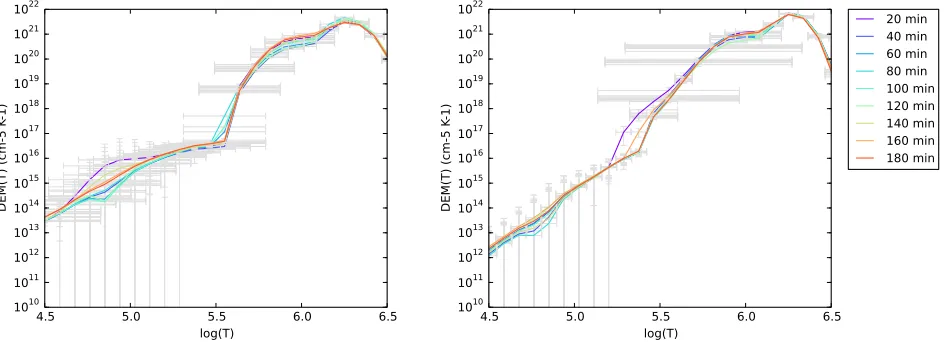
solu-tion. This is then solved by diagonalising the matri-ces R and L using generalised singular value decompo-sition, with the 1/λ term in the resulting expression ef-fectively smoothing the solution by filtering out small singular components. To implement the steps above, we use the DEM regularisation method by Hannah & Kontar (2012), which we adapted to Python program-ming language. We run the DEM regularisation using the SDO/AIA data in the same bandpasses as above av-eraged over the region of interest shown in Figure 8. We further averaged the data over 20 time frames to increase signal-to-noise ratio. We reconstruct the DEM for a tem-perature range between logT = 4.5 and logT = 7.3 and further apply additional constraint on DEM by requiring

it to be positive. Time evolution of the resulting DEM is shown in Figure 10.

The prominent DEM peak is centred around logT = 6.0. We are most concerned with the DEM evolution be-low logT = 6.0, especially with the secondary peak that develops around logT = 5.0. The amount of plasma in the transition region temperature increases during the first 50 min of the observation coinciding with the time interval of the coronal rain occurrence in the upper part of the loop. It should however be noted that the validity of the DEM inversion is based on the implicit assump-tion of the optically thin emission, the resulting DEM evolution in the lower end of the analysed temperature range should therefore be treated with caution.

Given that the 304 ˚A channel is most likely to be sen-sitive to optically thick emission, we repeated the DEM inversion without using the 304 ˚A channel (Figure 10). This mostly affects the evolution of the low-temperature region, with the early time peak shifted to logT = 5.5. Aside from that the overall shape remains similar. Fig-ure 11 shows the evolution of the DEM integrated along the whole temperature range (representing the evolution of the total amount of plasma at the loop top) and the intensity in the IRIS Si IV time-distance plot correspond-ing to the slit at the apex (as shown in Figure 3) averaged in transverse direction. The linear correlation coefficients between the Si IV emission intensity and EM recovered with and without using the 304 channel are 0.41 and

−0.10 respectively. When including the 304 channel the overall amount of plasma correlates well with the evo-lution of the emission in Si IV line, with matching time scales on which the quasi-periodic large scale variations occur. In the second case no clear correlation is present. We therefore conclude that due to its broad temperature response the 304 channel can help to better constrain the DEM in the lower temperature range.

The DEM reconstruction and the evolution of the in-dividual light curves together with the occurrence of suc-cessive coronal rain events in the same loop suggest that the observed sequence is a part of a continuously repeat-ing heatrepeat-ing-condensation cycle, consistrepeat-ing of a heatrepeat-ing phase, followed by radiative cooling of the loop top lead-ing to the thermally unstable regime and subsequent con-densation of the plasma, which is then followed by an-other heating phase.

4.5 5.0 5.5 6.0 6.5 log(T)

1010

1011

1012

1013

1014

1015

1016

1017

1018

1019

1020

1021

1022

DE

M(

T)

(cm

-5

K-1

)

4.5 5.0 5.5 6.0 6.5

log(T) 1010

1011

1012

1013

1014

1015

1016

1017

1018

1019

1020

1021

1022

DE

M(

T)

(cm

-5

K-1

)

20 min 40 min 60 min 80 min 100 min 120 min 140 min 160 min 180 min

Figure 10. Evolution of the regularised DEM plotted every 100 time steps including (left) and (right) excluding the 304 ˚A channel.

0 50 100 150 200

time (min) 4.5

5.0 5.5 6.0 6.5 7.0 7.5 8.0 8.5

EM

(c

m-5)

1e27

EM EM w/o 304 Å IRIS 1400 Å

−4 −2 0 2 4

Int

en

sit

y (

DN

)

Figure 11. Evolution of the emission measure integrated along the whole temperature range (red) and of the Si IV emission inten-sity in the time-distance plot corresponding to the slit at the loop apex (blue). The solid and dashed lines show the emission measure recovered with and without using 304 ˚A channel respectively. All time series have been smoothed for clarity. The data gap in Si IV emission time series corresponds to the SAA-contaminated data.

ξ(T) =ξ0(T) exp(

−(logT−logT0)2

2σ2 ) (5)

where ξ0(T) ∝n2ez is the peak emission measure de-pendent on the electron density and the line-of-sight in-tegration depth, which we estimate to be of the order of 1 Mm, σ = 0.1 and logT0 is the mean temperature

of the loop plasma. log T0 evolves according to a

pro-cess consisting of a heating stage characteristic by a lin-ear increase in temperature up to maximum value of logT = 6.0, catastrophic cooling stage associated with the coronal rain formation where the temperature de-creases exponentially and a final gradual cooling stage down to logT = 5.0 (Figure 12). The evolution of the plasma density is modelled in a similar manner to vary linearly between logne = 9.0 and logne= 9.4 but with the peak slightly delayed, as shown in Figure 12. The initial and peak values were chosen based on typical val-ues expected in active region coronal loops. No direct correlation between the plasma temperature and density is explicitly assumed due to hydrostatic non-equilibrium being the fundamental characteristic of the footpoint-heated loops likely to undergo catastrophic cooling. This evolution effectively marks 3 distinct phases in the cycle: 1. heating with chromospheric evaporation associated

with increasing T and ne, 2. radiative cooling followed by thermal instability and plasma condensation associ-ated with decreasing T and increasingneand 3. further cooling accompanied by evacuation of the plasma at the loop top associated with decreasingT andne.

0 50 100 150 200 time (min)

0 200000 400000 600000 800000 1000000

T (

K)

108

109

1010

N

(cm

-3)

4.5 5.0 5.5 6.0 6.5 7.0 7.5

log(T) 104

106

108

1010

1012

1014

1016

1018

1020

1022

DE

M

(cm

-5

K-1

)

Figure 12. Left: Evolution of the mean temperatureT0(solid line) and density (dashed line) of the plasma at the loop top used to generate

the DEM model. The coloured sections mark the individual phases of the loop thermal cycle: Heating (red), condensation (yellow) and evacuation (blue). Right: The DEM model att= 0 used to calculate simulated intensities is shown in red. The individual components (constant CHIANTI active region DEM and Gaussian DEM corresponding to the loop plasma) are shown by the dashed line.

0

50

100

150

200

time (min)

10

10

10

Int

en

sit

y (

DN

s-1 p

x-1

)

0

50

100

150

200

time (min)

10

10

10

Int

en

sit

y (

DN

s-1 p

x-1

)

94

131

171

193

211

304

335

0

50

100

150

200

time (min)

0.85

0.90

0.95

1.00

1.05

1.10

1.15

1.20

1.25

Int

en

sit

y/

Av

g i

nte

nsi

ty

0

50

100

150

200

time (min)

0.90

0.95

1.00

1.05

1.10

1.15

Int

en

sit

y/

Av

g i

nte

nsi

ty

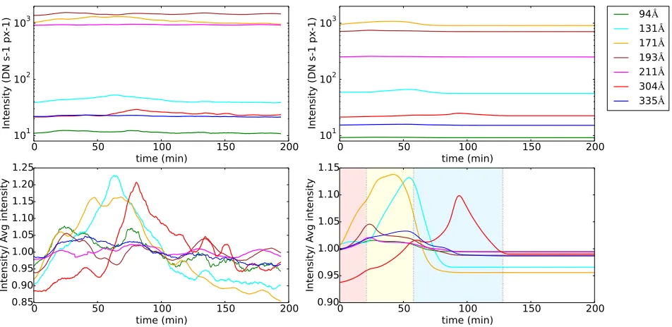
Figure 13. Comparison of the observed (left) and simulated emission intensities based on a 2 component DEM model corresponding to a simple heating-cooling process (right). The linear trend from the observed emission in 193 ˚A and 211 ˚A channels has been removed. Bottom panels show the emission intensities normalised by the average number of counts. The coloured sections mark the individual phases of the loop thermal cycle: Heating (red), condensation (yellow) and evacuation (blue).

the decay of all light curves is more rapid than observed. Here it should be noted that the DEM model used is valid for a monolithic loop. Multithermal structure of the coronal loop would result in greater width of the emission peaks, in line with the observations. Consider-ing above limitations of the background model and the fact that at lower temperatures the plasma is likely en-tering the optically thick regime, the forward modelling approach should be viewed as a demonstration of the fea-sibility of the limit cycle model given the observed light curve evolution rather than as a direct reproduction of the observations.

6. DISCUSSION

There is a number of possible sources that could po-tentially be responsible for the two distinct oscillation regimes with different periods. The 3.4 min average pe-riod characteristic for the small scale oscillation regime

is consistent with the period of the fundamental stand-ing modeP ≈√2L/vA∼3 min if using typical estimate for the Alfv´en speed (∼ 1000 km s−1) and loop length determined previously (129 Mm). Absence of observable damping in the small scale case suggests a presence of a continuously operating non-resonant driver. The mean period of the large scale oscillation regime is much longer than one expected for the fundamental harmonic and therefore cannot be associated with the standing mode scenario, suggesting the agent instead being a propagat-ing wave. Here the intermittent nature of the oscillations implies localised, transient driving mechanism operating near the foot points of the coronal loop.

events were found to excite transverse oscillations in the coronal loops with the periods on the order of minutes (Aschwanden et al. 2002; Nakariakov et al. 2009), match-ing the time scale of the small scale oscillation regime observed and discussed in this work. However, event-triggered loop oscillations usually exhibit strong damp-ing and were found to typically decay within few oscilla-tion periods (Nakariakov et al. 1999; White & Verwichte 2012), unlike the oscillations described here. There were no detected flares or other energetic events occurring on the date of the observation near AR 12151. An M class flare occurred in this active region during the previous day and a series of C class flares was observed in AR 12149 and AR 12150 on the day of observation; these were however perceived as being too distant to have a significant effect on the studied coronal loop. The limited STEREO-A dataset available for the day of observation was also checked to exclude the possibility of a nearby flare occurring behind the limb.

The persistent nature of the small scale oscillations and their lack of observable decay instead suggests that there is a possible link with the decayless transverse oscilla-tions of coronal loops in non-flaring active regions hav-ing similar characteristics which were observed at EUV wavelengths (e.g. Nistic`o et al. 2013). If the small scale oscillation regime is indeed a manifestation of the same process as these decayless loop oscillations, the common occurrence of this phenomenon implies a global nature of the driving mechanism; possibly a stochastic driver (e.g. small scale reconnection events or stochastic mo-tions in the chromospheric network resulting from gran-ular flows). Another possibility is a global helioseismic p-mode coupling to the loop footpoints. Because of the large number of other loops in the vicinity of the studied coronal loop, a possibility of an interaction with neigh-bouring loops has to be taken into account. Assuming that their proximity is not just a projection effect, in-teraction with the neighbouring loops could perturb the conditions in the studied loop and trigger both condensa-tion region formacondensa-tion and transverse loop oscillacondensa-tions. It has also been suggested that if the inertia of the coronal rain blobs is not negligible the condensations themselves could excite the oscillations in the loop. Detailed analysis of this scenario will be addressed in the future work.

The reasons behind sub-ballistic fall rates of the coro-nal rain blobs are less clear and subject to ongoing discus-sion. Gas pressure gradients in the loop are thought to have strong effect on the dynamics of plasma condensa-tions. As the condensation falls down along the magnetic field line, it compresses the plasma below. The resulting strong pressure could slow down the blob significantly. Numerical simulations show that these pressure effects can be strong enough to account for some of the observed deceleration (M¨uller et al. 2005; Fang et al. 2013; Oliver et al. 2014). The motion of the blobs would also appear sub-ballistic if the blobs would be moving along paths resulting from helical structure of magnetic field lines. Such helical configuration of the magnetic field would however need to be stable for extended periods of time which we consider unlikely. Another factor that needs to be considered is the ponderomotive force (PMF) exerted by the transverse oscillations in the loop. The PMF can be directed either along or against the direction of the motion of the condensations depending on their position

along the loop and on the harmonic of the transverse standing wave in the loop. This would provide an expla-nation the multiple acceleration and deceleration phases in the blob motion. The scenario that the coronal rain evolution is at least partially affected by the PMF is fur-ther supported by the fact that a number of coronal rain blobs was observed to oscillate around the loop top, as shown in Figure 5. Model of the effect of the PMF on the kinematics of the coronal rain has already been proposed (Verwichte et al. 2016, in prep.). The influence of the PMF on the coronal rain kinematics will be addressed in detail in the future work.

Our observations of the thermal evolution of the plasma in the studied coronal loop are consistent with the limit cycle model, where steadily heated loops are expected to undergo periodically repeating cycles con-sisting of heating and condensation phases with the pe-riods on the time scales of hours, typically dependent on the loop length and the shape of the heating function. A possibility of cyclic evolution of coronal loops was first addressed by Kuin & Martens (1982) who obtained an os-cillatory solution if the strength of the coupling between the coronal loop and the chromosphere was lower than a critical value, using a relatively simple semi-analytical model based on modelling the loop as a 0-dimensional system. Their model was further generalised by Gomez et al. (1990) by fully accounting for the hydrodynamic considerations whose solution has the form of subcriti-cal Hopf bifurcation. These models are of course highly simplified and use average values of the temperature and density along the loop, hence they do not account for a variation in the spatial distribution of the heating func-tion, which we now know is an important factor that determines the thermal instability onset. They can be however still used for prediction of the general behaviour of the system, since they account for key ingredients of the heating-condensation cycle: chromospheric evapora-tion, catastrophic cooling and subsequent evacuation of the loop. The limit cycle behaviour has been also pre-dicted by a number of numerical studies (e.g. Karpen et al. 2001; M¨uller et al. 2003; Fang et al. 2015).

0.0

0.2

0.4

0.6

0.8

1.0

T (K)

1e6

0.8

1.0

1.2

1.4

1.6

1.8

2.0

2.2

2.4

2.6

N

(cm

-3)

1e9

Evacuation

Condensation

Heating

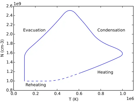
Reheating

Figure 14. Phase diagram of the loop evolution deduced from forward modelling the SDO/AIA emission intensities. The dashed line shows extrapolated evolution prior to the start of the observa-tional sequence.

cooler bandpasses), given the lack of a simple observa-tional signature of the presence of a heating phase im-mediately preceding the cooling of the loop plasma. The deduced effect of adding the heating phase on the on-set of cooling progression when forward modelling the emission intensities however seems to be in line with the observations. This, together with the repeated coronal rain occurrences in the same coronal loop supports the complete heating-condensation cycle scenario.

Whereas the resulting DEM evolution calculated using the regularisation method is in agreement with the re-sults deduced using the forward modelling approach, care must be taken with the interpretation of the thermal evo-lution of the plasma in the lower end of the analysed tem-perature range, where it is likely entering the optically thick regime. In addition, contamination of the emission from the studied region by the emission of the hot coronal background seems to be an ongoing problem. In order to evaluate the degree to which the DEM determined in this work is affected by the coronal background, it should be pointed out that due to the greater column depth, the contamination by the background emission is likely to be more severe near the solar limb than near the centre of the solar disk, where the DEM is usually much more ac-curate (e.g. Warren et al. 2010; Hannah & Kontar 2012). Since the coronal rain is best observed off-limb, this poses a challenge for the extraction of the relevant information about temperature evolution of the studied coronal loop. The background subtraction was not carried out in this work, as it proved impossible to select a reference area where the average intensity in the most noisy channels (94 ˚A and 335 ˚A) would be less than the average value in the analysed region in all time frames. An alternative approach would be to simply exclude these two channels from the analysis. However, this was viewed as unde-sirable due to the fact that it would lead to the DEM being even more under-constrained. Including the effect of the hot coronal background and tackling the problem using the forward modelling therefore seems to be the most viable approach for the off-limb regions. However, as shown by this work, the steady background model has its limitations, since a change in the background

tem-perature during the period of the observation (e.g. due to a bundle of loops undergoing similar heating-cooling cycles, but with longer cycle periods) is entirely possible. The change of plasma density near the loop top result-ing from the chromospheric evaporation and subsequent condensation is expected to have an effect on the Alfv´en speed in this part of the loop. For the change in density by a factor of 2.5 as estimated in the previous section, the Alfv´en speed vA =B/√µ0ρ is expected to change by a

factor of 1.6. Withvph≈√2vAandvph=λ/P, this de-crease in density will result in dede-crease in the oscillation period by a factor of 1.6 and vice versa. The observed scatter in the period of the oscillations traced by the coronal rain blobs could therefore be partially caused by the density change due to evacuation of the loop top.

7. CONCLUSIONS

We analysed transverse oscillations and kinematics of coronal rain observed by IRIS, Hinode/SOT and SDO/AIA. Two different regimes of transverse oscilla-tions traced by the rain in the studied coronal loop were observed: small-scale oscillations with mean period of 3.4 min and amplitudes between 0.2-0.4 Mm that can be observed along the whole loop length and large-scale oscillations with mean period 17.4 min and amplitudes around 1 Mm, observable only in the lower part of the loop. The small scale oscillations are visible during most of the duration of the dataset without any observable damping, they are therefore likely driven by a continu-ously operating process. The collective behaviour of the individual oscillating strands and lack of phase shift sug-gests they correspond to a standing wave excited along the whole loop. The 3.4 min period of this oscillation regime is consistent with period expected for a funda-mental harmonic of the loop with similar length. The large scale oscillations are only visible in the latter half of the observational sequence. The unusually long period suggests a propagating wave scenario, where the wave is excited by a transient mechanism localised near the loop foot points.

Plasma condensations were found to move with speeds ranging from few km s−1 up to 180 km s−1 and with accelerations that were largely below the free fall rate. The broad velocity distribution, sub-ballistic motion and complex velocity profiles of individual blobs showing mul-tiple acceleration and deceleration phases suggest that forces other than gravity have significant effect on the evolution of the coronal rain, the likely candidates being pressure effects and the ponderomotive force caused by the transverse loop oscillations.

P.K. would like to acknowledge the support of the UK STFC PhD studentship. E.V. acknowledges financial support from the UK STFC on the Warwick STFC Con-solidated Grant ST/L000733/I. We would like to thank P. Antolin, G. Vissers and D. Yuan, the co-observers dur-ing the August 2014 observdur-ing campaign at SST. This research has made use of SunPy, an open-source and free community-developed solar data analysis package written in Python (http://sunpy.org). IRIS is a NASA small explorer mission developed and operated by LM-SAL with mission operations executed at NASA Ames Research center and major contributions to downlink communications funded by the Norwegian Space Cen-ter (NSC, Norway) through an ESA PRODEX contract. Hinode is a Japanese mission developed and launched by ISAS/JAXA, with NAOJ as domestic partner and NASA and STFC (UK) as international partners. It is operated by these agencies in co-operation with ESA and NSC (Norway). The SDO/AIA data are available by courtesy of NASA/SDO and the AIA, EVE, and HMI science teams. The work was also supported by the in-ternational programme “Implications for coronal heating and magnetic fields from coronal rain observations and modelling” of the International Space Science Institute (ISSI), Bern.

REFERENCES

Anfinogentov, S., Nistic`o, G., & Nakariakov, V. M. 2013, A&A, 560, A107

Antolin, P., Okamoto, T. J., Pontieu, B. D., et al. 2015a, ApJ, 809, 72

Antolin, P., & Rouppe van der Voort, L. 2012, ApJ, 745, 152 Antolin, P., Shibata, K., & Vissers, G. 2010, ApJ, 716, 154 Antolin, P., & Verwichte, E. 2011, ApJ, 736, 121

Antolin, P., Vissers, G., Pereira, T. M. D., Rouppe van der Voort, L., & Scullion, E. 2015b, ApJ, 806, 81

Antolin, P., Vissers, G., & Rouppe van der Voort, L. 2012, Sol. Phys., 280, 457

Aschwanden, M. J., Fletcher, L., Schrijver, C. J., & Alexander, D. 1999, ApJ, 520, 880

Aschwanden, M. J., Pontieu, B. D., Schrijver, C. J., & Title, A. M. 2002, Sol. Phys., 206, 99

Aschwanden, M. J., Schrijver, C. J., & Alexander, D. 2001, ApJ, 550, 1036

Auch`ere, F., Bocchialini, K., Solomon, J., & Tison, E. 2014, A&A, 563, A8

Berger, T., Testa, P., Hillier, A., et al. 2011, Nature, 472, 197 Boerner, P., Edwards, C., Lemen, J., et al. 2011, Sol. Phys., 275,

41

De Groof, A., Bastiaensen, C., M¨uller, D. A. N., Berghmans, D., & Poedts, S. 2005, A&A, 443, 319

De Groof, A., Berghmans, D., van Driel-Gesztelyi, L., & Poedts, S. 2004, A&A, 415, 1141

De Pontieu, B., Title, A. M., Lemen, J. R., et al. 2014, Sol. Phys., 289, 2733

Dere, K. P., & Mason, H. E. 1993, Sol. Phys., 144, 217 Edwin, P. M., & Roberts, B. 1983, Sol. Phys., 88, 179 Fang, X., Xia, C., & Keppens, R. 2013, ApJL, 771, L29

Fang, X., Xia, C., Keppens, R., & Doorsselaere, T. V. 2015, ApJ, 807, 142

Foullon, C., Verwichte, E., & Nakariakov, V. M. 2004, A&A, 427, 4

—. 2009, ApJ, 700, 1658

Froment, C., Auch`ere, F., Bocchialini, K., et al. 2015, ApJ, 807, 158

Gomez, D., Sicardi Schifino, A., & Ferro Fontan, C. 1990, ApJ, 352, 318

Goossens, M., Andries, J., & Aschwanden, M. J. 2002, A&A, 394, L39

Goossens, M., Erd´elyi, R., & Ruderman, M. S. 2010, Space Sci. Rev., 158, 289

Goossens, M., Terradas, J., Andries, J., Arregui, I., & Ballester, J. L. 2009, A&A, 503, 213

Hannah, I. G., & Kontar, E. P. 2012, A&A, 539, A146 Hershaw, J., Foullon, C., Nakariakov, V. M., & Verwichte, E.

2011, A&A, 531, A53

Hollweg, J. V., & Yang, G. 1988, J. Geophys. Res., 93, 5423 Kamio, S., Peter, H., Curdt, W., & Solanki, S. K. 2011, A&A,

532, A96

Karpen, J. T., Antiochos, S. K., Hohensee, M., Klimchuk, J. A., & MacNeice, P. J. 2001, ApJ, 553, L85

Kawaguchi, I. 1970, PASJ, 22, 405

Kleint, L., Antolin, P., Tian, H., et al. 2014, ApJ, 789, L42 Kuin, N. P. M., & Martens, P. C. H. 1982, A&A, 108, L1 Lemen, J. R., Title, A. M., Akin, D. J., et al. 2012, Sol. Phys.,

275, 17

Leroy, J.-L. 1972, Sol. Phys., 25, 413

Marsch, E., Tian, H., Sun, J., Curdt, W., & Wiegelmann, T. 2008, ApJ, 685, 1262

Mart´ınez Oliveros, J.-C., Krucker, S., Hudson, H. S., et al. 2014, ApJ, 780, L28

McIntosh, S. W., De Pontieu, B., Carlsson, M., et al. 2011, Nature, 475, 477

McIntosh, S. W., Tian, H., Sechler, M., & Pontieu, B. D. 2012, ApJ, 749, 60

M¨uller, D. A. N., De Groof, A., Hansteen, V. H., & Peter, H. 2005, A&A, 436, 1067

M¨uller, D. A. N., Hansteen, V. H., & Peter, H. 2003, A&A, 411, 9 M¨uller, D. A. N., Peter, H., & Hansteen, V. H. 2004, A&A, 424,

12

Nakariakov, V. M., Aschwanden, M. J., & van Doorsselaere, T. 2009, A&A, 502, 661

Nakariakov, V. M., Ofman, L., Deluca, E. E., Roberts, B., & Davila, J. M. 1999, Science, 285, 862

Nakariakov, V. M., & Verwichte, E. 2005, Liv. Rev. Sol. Phys., 2, 3

Nistic`o, G., Nakariakov, V. M., & Verwichte, E. 2013, A&A, 552, A57

Okamoto, T. J., Antolin, P., Pontieu, B. D., et al. 2015, ApJ, 809, 71

Oliver, R., Soler, R., Terradas, J., Zaqarashvili, T. V., & Khodachenko, M. L. 2014, ApJ, 784, 21

Ruderman, M. S., & Roberts, B. 2002, ApJ, 577, 475 Schrijver, C. J. 2001, Sol. Phys., 198, 325

Scullion, E., Rouppe van der Voort, L., Wedemeyer, S., & Antolin, P. 2014, ApJ, 797, 36

Tikhonov, A. N. 1963, Soviet Math. Dokl., 4, 1035

Tomczyk, S., McIntosh, S. W., Keil, S. L., et al. 2007, Science, 317, 1192

Tsuneta, S., Ichimoto, K., Katsukawa, Y., et al. 2008, Sol. Phys., 249, 167

Ugarte-Urra, I., Warren, H. P., & Brooks, D. H. 2009, ApJ, 695, 642

Ugarte-Urra, I., Winebarger, A. R., & Warren, H. P. 2006, ApJ, 643, 1245

Van Doorsselaere, T., Nakariakov, V. M., & Verwichte, E. 2008, ApJL, 676, L73

Verwichte, E., Aschwanden, M. J., Doorsselaere, T. V., Foullon, C., & Nakariakov, V. M. 2009, ApJ, 698, 397

Verwichte, E., Foullon, C., & Doorsselaere, T. V. 2010, ApJ, 717, 458

Wang, T., Ofman, L., Davila, J. M., & Su, Y. 2012, ApJ, 751, L27 Warren, H. P., Winebarger, A. R., & Brooks, D. H. 2010, ApJ,

711, 228

White, R. S., & Verwichte, E. 2012, A&A, 537, A49

White, R. S., Verwichte, E., & Foullon, C. 2012, A&A, 545, A129 Williams, D. R., Phillips, K. J. H., Rudawy, P., et al. 2001,

MNRAS, 326, 428