The applicability of the ASED sensor for measuring bed level changes in intertidal areas

Full text

(1)Master Thesis The applicability of the ASED-sensor for measuring bed level changes in intertidal areas.

(2)

(3) MASTER THESIS IN WATER ENGINEERING AND MANAGEMENT FACULTY OF ENGINEERING TECHNOLOGY UNIVERSITY OF TWENTE. April 18, 2019. Author: Student number: Location: Organization:. A. (Anja) Mus s1871587 Enschede and Yerseke University of Twente and Royal Netherlands Institute of Sea Research (NIOZ). Graduation committee: University of Twente Ir. P.W.J.M. Willemsen Dr. Ir. B.W. Borsje Prof. Dr. S.J.M.H. Hulscher Experimental support: NIOZ. Prof. Dr. T.J. Bouma J. van Dalen.

(4)

(5) Preface This report is the final product of my master thesis in the Water Engineering and Management (WEM) department of the University of Twente and Royal Netherlands Institute of Sea Research (NIOZ). The research is executed under the supervision of Prof. Dr. T.J. Bouma, J. van Dalen from NIOZ, Prof. Dr. S.J.M.H. Hulscher, Dr. Ir. B.W. Borsje and Ir. P.W.J.M. Willemsen of the University of Twente. The major part of the study was conducted at the University of Twente, whereas lab and field experiments were executed during a period of one month at NIOZ in Yerseke. Finishing this report marks the end of my time as a student, which I have very much enjoyed over the past years. I have had great experiences and met wonderful people and would like to thank everyone involved in this period of my life. This report could not have been made without the help of some people. Firstly, I would like to thank my supervisors, with in particular P.W.J.M. Willemsen for the weekly support and revisions during the study. Furthermore, I would also like to thank F. van Maarseveen and B. Denissen for explaining the ASED-sensor in detail, R. Maaskant for helping me through the entire process, and H. Maaskant for reviewing my report during the final stages of the thesis..

(6)

(7) Abstract The Acoustic Sediment Elevation Dynamics (ASED)-sensor is a stand-alone measuring device designed by NIOZ, to study bed level dynamics within intertidal areas. The ASEDsensor was used to study the morphological behaviour of intertidal flats. However, the sensor was not yet properly tested and lacked an algorithm and autonomous script for translating raw intensity data into bed level data. Therefore, the objective of this study is to assess the applicability of the ASED-sensor for measuring bed level changes in intertidal areas. It includes developing the raw data processing algorithms and their implementation in Python scripts. The ASED-sensor uses a pulsed acoustic signal of approximately 300 kHz to measure bed levels during submerged conditions. The reflected signal by the bed is detected by a sudden increase in amplitude. The travel time of the signal from the sensor to the bed and vice versa needs to be converted to a distance, to obtain bed levels. The sensor will be tested both in the lab and in the field. Lab experiments need to be collected to verify whether the ASED-sensor can detect the echo and measure the travel time in a range of environmental conditions in the water tank and wave flume at NIOZ in Yerseke. The environmental conditions consisted of water depths, soil types, dilutions of soil types, and waves and current forcing. Thereafter the ASED-sensor was deployed to measure in the field. The field experiments were performed in the Eastern Scheldt, next to NIOZ, and in the Western Scheldt at the Kapellebank. The Eastern Scheldt experiment was performed during a weekend, while the Western Scheldt experiment collected data for 19 days. The lab experiments and the Eastern Scheldt experiment were validated with a manual measurement using a tape measure. The validation of the Western Scheldt experiment’s data was accomplished by a tape measure and erosion pins. At the start of the study, the ASED-sensor lacked an autonomous script for translating raw intensity data into bed level data. Therefore, three algorithms were tested, consisting of Fast Fourier Transform, envelope method and the Kalman filter. The Kalman filter method showed the most promising results, with the lowest standard deviation and lowest computation time. Parameter settings within the script were determined using the lab and field experiments. The parameter settings are filtering noise and searching the start of the sudden increase in amplitude of the first strong signal reflected by the bed. These parameters tune the bed detection of the ASED-sensor. The practical measurement domain for the ASED-sensor is from 0.20 m to 0.45 m, according to the raw data analysis of all lab experiments. The coefficient of determination (𝑅 2) between the newly developed script and the manual measurements was 0.99 for the lab experiments. The bed could be detected during the field experiments. The actual accuracy is 2 mm to 4 mm, obtained from the lab experiments. The predecessor Sediment Elevation Dynamics (SED)-sensor scores 4 mm for the accuracy (De Mey, 2016). The light cells based SED-sensor cannot measure during nocturnal and submerged conditions. The hydrodynamics are only active during submerged conditions and thus morphological changes cannot be observed by the SED-sensor but can be observed by acoustic instruments. Most acoustic instruments have the same accuracy but have a high unit cost and labour-intensive deployments. The ASED-sensor, with its high vertical accuracy, low labour-intensive deployment cost and reasonable cost, is well suited for monitoring bed level dynamics in intertidal areas..

(8) List of abbreviations ADCP ADV ASED-sensor FFT GNSS GPS MBES NIOZ PEEP-sensor RPM RTK SBES SED-sensor SSC WEM. Acoustic Doppler Current Profiler Acoustic Doppler Velocimeter Acoustic Sediment Elevation Dynamics sensor Fast Fourier Transform Global Navigate Satellite System Global Positioning System Multi Beam Echo Sounder Royal Netherlands Institute of Sea Research Photo-Electronic Erosion Pin sensor Rotation Per Minute Real Time Kinematic Single Beam Echo Sounder Sediment Elevation Dynamics sensor Suspended Sediment Concentration Water Engineering and Management.

(9) Contents 1. INTRODUCTION......................................................................................................................... 1 1.1 1.2 1.3 1.4 1.5. 2. METHODS .................................................................................................................................... 5 2.1 2.2 2.3 2.4. 3. THE ASED SENSOR.................................................................................................................. 5 STUDY SITES ............................................................................................................................ 8 LAB AND FIELD EXPERIMENTS ............................................................................................... 11 CONVERTING RAW DATA TO BED LEVELS................................................................................ 15. RESULTS .................................................................................................................................... 22 3.1 3.2 3.3 3.4. 4. BACKGROUND .......................................................................................................................... 1 RESEARCH GAP AND RELEVANCE ............................................................................................. 3 RESEARCH OBJECTIVE ............................................................................................................. 4 RESEARCH QUESTIONS ............................................................................................................. 4 REPORT OUTLINE ..................................................................................................................... 4. MEASURING WITH THE ASED-SENSOR .................................................................................. 22 COLLECTING RAW DATA ......................................................................................................... 23 CONVERTING RAW DATA TO BED LEVEL DATA ........................................................................ 30 THE ACCURACY OF THE ASED-SENSOR ................................................................................. 42. DISCUSSION.............................................................................................................................. 43 4.1 4.2 4.3 4.4 4.5 4.6. MEASURING WITH THE ASED-SENSOR .................................................................................. 43 COLLECTING RAW DATA ......................................................................................................... 45 CONVERTING RAW DATA TO BED LEVEL DATA ........................................................................ 46 COMPARISON WITH THE SED-SENSOR ................................................................................... 48 FURTHER POSSIBILITIES ASED-SENSOR ............................................................................... 49 EXTRA MEASUREMENTS ......................................................................................................... 50. 5. CONCLUSIONS ......................................................................................................................... 51. 6. RECOMMENDATIONS ............................................................................................................ 52. A. APPENDICES ............................................................................................................................ 57 A.1 A.2 A.3 A.4 A.5 A.6 A.7 A.8 A.9. ASED-SENSOR ....................................................................................................................... 57 SEDIMENT DISTRIBUTION....................................................................................................... 65 FLUME CALIBRATION ............................................................................................................. 66 SSC LAB EXPERIMENT ........................................................................................................... 67 ANALYSED METHODS ............................................................................................................. 69 FORMULAS OF THE SPEED OF SOUND ..................................................................................... 78 EXTRA RESULTS EXPERIMENTS .............................................................................................. 82 INUNDATIONS OF THE FIELD EXPERIMENTS ........................................................................... 87 PERFORMED EXPERIMENTS .................................................................................................... 90.

(10)

(11) 1 Introduction 1.1 Background The ability of salt marshes and tidal mudflats to aggrade vertically to maintain their position in the intertidal region has been the focus of numerous studies over the last 50 years (Ranwell, 1964; Leonard et al., 1995; Möller et al., 2014). During the present era of sea-level rise and increasing storminess, sustainable coastal protection requires in-depth understanding of their long-term lateral dynamics and their ability to survive the changing conditions (Callaghan et al., 2010; Yang et al., 2012; Bouma et al., 2014; Möller et al., 2014). Coastal ecosystems, such as tidal flats and salt marshes (Figure 1.1), mangrove forests and reefs, can contribute to coastal protection and flood risk reduction by surge attenuation (Wamsley et al., 2010), wave energy dissipation and erosion reduction (Gedan et al., 2011).. Figure 1.1: Exposed, sand-rich tidal flat and salt marsh (Friedrichs, 2012). The morphological evolution (i.e., the balance between erosion and accretion) of tidal flats and salt marshes are influenced by tidal currents and waves (van der Wal et al., 2008; Callaghan et al., 2010). Morphodynamical changes in salt marshes are suppressed by vegetation, but dynamics at tidal flats occur much faster due to the absence of vegetation (Möller et al., 1999; Hu et al., 2015). Three different types of measurements showed, that sediment deposition occurred on the marsh surface during rising tides at tidal elevations ranging from those barely flooding the creek bank to high spring tides, and that sediment was not remobilized by tidal flows after initial deposition (Christiansen et al., 1999). Flooding is the main mechanism for sediment delivery to the marsh platform, salt marshes are therefore inevitably linked to sea level and tidal oscillations (Fagherazzi et al., 2012). Sediment deposition occurred on the marsh surface largely because fine sediment in suspension formed flocs. The processes controlling sediment deposition did not vary among tides. However, Suspended Sediment Concentration (SSC) near the creek bank increased with increasing tidal amplitude, consequently promoting higher rates of deposition with higher tides (Christiansen et al., 1999). If vertical sediment accretion is smaller than sea-level rise, marshes are at risk of drowning and suffer “coastal squeeze” when dykes prevent (high) marshes to recede inland (Doody, 2004). Besides all this, there is a seasonal influence of waves on the shore and mudflats. Winter has higher waves whereby the sediment is placed further outwards and the beach becomes steeper. The beach steepness is low in summer, due to the calmer waves and more deposition of sand on the beach. High hydrodynamic energy either from waves or current velocity, and lack of sediment will generally cause mudflat–salt marsh ecosystems to reduce in size due to erosion. The. Page 1 of 90.

(12) inverse, high sediment availability combined with low hydrodynamic energy, most likely results in vertical accretion and/or lateral extension (Bouma et al., 2005, 2016). The waves and current forcing generate bottom shear stresses, which are relevant for sediment erosion and deposition. The bottom shear stress at the bed is a combined effect of nonlinear interactions between the mean flow and the waves (Le Hir et al., 2000). As mentioned before the tidal flat topography is continuously shaped by hydrodynamic force from tidal currents and wind waves (Hu et al., 2015). As such forces have great temporal and spatial variability on short time scales, they may impose short-term surface elevation (Le Hir et al., 2000; Green et al., 2014). The short-term bed level change information is vital to identify the effect of current hydrodynamic forcing and to understand fundamental processes in sediment transport (Friedrichs, 2012; Green et al., 2014). Wave forcing is known to vary strongly with wave direction, wave period, wave height and tidal phase or water depth (Nielsen, 2009). Current forcing varies hourly with the tidal phase, and the tidal range varies fortnightly with the spring/neap cycle (Bouma et al., 2005). Waves and current field measurements on tidal flat and salt-marsh ecosystems indicated that the hydrodynamic forcing on the bottom sediment was strongly influenced by wind-generated waves, more so than by tidal- or wind-driven currents (Callaghan et al., 2010). The measurements further showed that the hydrodynamic forcing decreased considerably landward of the marsh cliff, highlighting a transition from vigorous (tidal flat and pioneer zone) to sluggish (mature marsh) fluid forcing (Callaghan et al., 2010). Within the estuarine and coastal environment, tidal flats and salt marshes play an important role as essential habitats for plants and animals and as sinks and/or source for nutrients, pollutant and sediment (Figure 1.1; Allen, 2000; Doody, 2004). They also play a significant role in coastal defence, enhancing coastal sedimentation, as the intertidal vegetation decreases water movements and binds sediments (USACE, 1989). Sedimentrich environments with gentle bed slopes are a common representation of the tidal flats (Figure 1.1; Friedrichs, 2012). The vegetation in salt marshes ensures a stable sediment bed. Despite the absence of vegetation in the tidal flat, bed level changes are influenced by ecology, due to the seasonal presence of stabilizers and destabilizers bio-engineers on tidal flats, like algal tufts for the stabilizing effect and lugworms for destabilizing (Volkenborn et al., 2008; Hu et al., 2015). The wave attenuation by vegetation generally causes an exponential decline of wave energy with distance across salt marshes (Bouma et al., 2005; Möller et al., 1999; Yang et al., 2012). Comparisons show that wave attenuation across salt marshes is determined by vegetation characteristics, hydrodynamics, and sediment bed and can show spatial and temporal variations (Yang et al., 2012). To identify the short-term bed level changes an instrument is needed which can monitor those changes. Several instruments such as: Photo-Electronic Erosion Pin (PEEP) sensor and the SED-sensor are used to measure bed level changes. A big limitation of these instruments is that they cannot measure during submerged and nocturnal conditions (Lawler, 2008; Hu et al., 2015). Another instrument, the electro-resistivity sensor, which uses the difference in the electrical conductivity of seawater and sediment, has a low (1030 mm) vertical resolution (Ridd, 1992; Hu et al., 2015). As alternative different acoustic instruments have been used, such as: ALTUS (Ganthy et al., 2013), Acoustic Doppler Velocimeter (ADV) (McLelland et al., 2000), Acoustic Doppler Current Profiler (ADCP) (Horstman et al., 2011), Single Beam Echo Sounder (SBES) (Kongsberg Maritime AS, 2017) and Multi Beam Echo Sounder (MBES) (Kongsberg, 2017). The acoustic instruments generally have the highest vertical resolution (within 2 mm). However, most of these Page 2 of 90.

(13) methods require external power and an on-site data-logging system, which leads to high unit cost and labour-intensive deployment (Hu et al., 2015). The acoustic instruments cost more than €8000. Conventional discontinuous surface-elevation monitoring typically has a coarse temporal resolution (weeks to months), determined by resurvey frequency (Lawler, 2008; Nolte et al., 2013). The NIOZ developed a new sensor called the ASED-sensor. The ASED-sensor is a standalone device, like the predecessor SED-sensor. The ASED-sensor measures the propagation time of the signal reflected by the bed using an acoustic signal with a measurement frequency of approximately 300 kHz (Appendix A.1.1). This allows the sediment dynamics to be measured continuously during submerged conditions (Thorne et al., 2002). This study is the first time that the ASED-sensor is tested thoroughly. First, the ASED-sensor will be validated during lab experiments before the data of the ASEDsensor can be trusted in the field.. 1.2 Research gap and relevance Estuarine tidal flats and salt marshes are important ecosystems, providing coastal protection (Allen, 2000; Callaghan et al., 2010). Hydrodynamic energy either from waves or current velocity and sediment will cause the salt marsh and tidal flat to laterally grow and retreat (Bouma et al., 2005). The size of the system influences the contribution to wave energy reduction and thereby on coastal protection (Vuik et al., 2016); therefore, it is important to monitor bed level changes. The morphological development of the bed is driven by the hydrodynamic characterisation of a mudflat-salt marsh ecosystem. Yet, there is not much known about the relationship between the hydrodynamics and the morphological changes of the seabed. Therefore, an instrument is needed to measure in high resolution these morphological changes to understand the underlying processes. Accordingly, NIOZ designed a novel stand-alone instrument called the ASED-sensor. The ASED-sensor detects sediment surface position by an acoustic signal and is developed to measure with a high vertical resolution. The ASED-sensor has a high battery and storage capacity. Therefore, the surface elevation dynamics can be measured with a high temporal resolution. The problem with the predecessor SED-sensor not continuously measuring during submerged conditions has been solved. It is important to measure during submerged conditions because the hydrodynamics are only active during submerged conditions and thus morphological changes can be observed. This sensor is relatively cheap compared to the other acoustic instruments and should have similar accuracy. Since the sensor is cheap, a network of ASED-sensors could be placed in intertidal areas to register not only temporal variations but also spatial variations.. Page 3 of 90.

(14) 1.3 Research objective The objective of this study is: Assessing the applicability of the ASED-sensor for measuring bed level changes in intertidal areas. Waves, currents and vegetation are the influencing factors for morphological changes (Möller, 2006). The bed level changes occur mostly during submerged conditions. For the registration of bed level changes, the ASED-sensor has been used. A script is built to convert the raw data into bed levels. This might improve the understanding of the underlying processes for the bed level changes during submerged conditions. Climate change, land subsidence and population growth in coastal areas lead to an increase in flood hazards and in its consequent economic damage and loss of life (Mendelsohn et al., 2011). The ASED-sensor, with its high vertical accuracy, low labour-intensive deployment cost and reasonable cost, is well suited for monitoring bed level dynamics in intertidal areas. Therefore, this study will give a better understanding of the short and long term morphodynamics using the ASED-sensor.. 1.4 Research questions Three research questions have been formulated to achieve the research objective. 1) What is the ASED-sensor? 2) For what range of environmental conditions can the ASED-sensor detect a bed? a) Under controlled lab experiments? i) The range of water depths? ii) The range of soil types? iii) The range of dilutions of the different soil types? iv) During waves and current forcing? b) During field experiments? i) In the Eastern Scheldt? ii) In the Western Scheldt? 3) What converting method is suitable for detecting the bed using the raw data of the ASED-sensor?. 1.5 Report outline Following this introductory chapter, the next chapter starts by explaining the ASEDsensor, describes the study sites for collecting the lab and field data and illustrates the methods for converting the raw data into bed levels. Consecutively, chapter 3 describes the results of the raw data of the ASED-sensor under several conditions and converting the raw data into bed levels. Thereafter discussions, conclusions and recommendations are provided in chapter 4, 5 and 6.. Page 4 of 90.

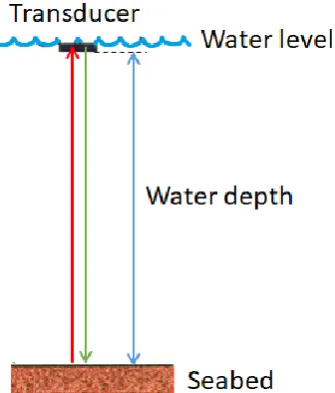
(15) 2 Methods 2.1 The ASED sensor The ASED-sensor is a stand-alone device that measures the propagation time of the signal reflected by the bed using an acoustic signal with a measurement frequency of approximately 300 kHz (Appendix A.1.1). The ASED-sensor has a storage capacity of 8 GB. The ASED-sensor has an energy supply from a battery pack of 8 alkaline AA battery cells (F. van Maarseveen, personal communication, October 15, 2018). The sensor is made waterproof by the transparent polyester case (Figure 2.1). The ASED-sensor has one transmitting transducer and one receiving transducer. The transducers are made waterproof by a 4 mm layer of lime/sealer 604 of Ruplo (F. van Maarseveen, personal communication, October 15, 2018). Between the transducers and the lime/sealer no air is present (Figure 2.2). The acoustic signal propagates from the transmitter through the water to the seabed (green arrow; Figure 2.3) and reflects at the seabed returning to the receiver (red arrow; Figure 2.3). Therefore, to define the water depth the signal travel time needs to be divided by two and multiplied by the speed of sound (blue arrow; Figure 2.3). The speed of sound varies by the water temperature, water pressure and the salinity. The ASED-sensor measures the water pressure, in 0.1 mbar accurate, and the water temperature, 2 decimals accurate in degrees Celsius. Salinity is determined independently, by conductivity sensor or from Rijkswaterstaat (Dutch department of waterways and public works) in parts per thousand. The time of measurement is recorded in milliseconds from 1-Jan-2001. The voltage of the battery, the start and the end voltage of the transmission are stored in millivolt (F. van Maarseveen, personal communication, October 15, 2018).. Figure 2.2: The head of the ASED-sensor with two transducers and the 4 mm thick lime/sealer.. Figure 2.1: The waterproof transparent polyester case of the ASED-sensor. Figure 2.3: Signal transmission through the water. Page 5 of 90.

(16) Before the signal can be sent into the water, the electric signal from the transducer needs to be transformed into an acoustic signal into the water and vice versa. The piezoelectric material in the transducer ensures these translations. First, the transducer’s analogue signal output is amplified and then passed through a bandpass-filter to lower the noise. It is then sampled at a 4 MHz sample rate with an 8bit accuracy (F. van Maarseveen, personal communication, October 15, 2018). During the transmission of the pulse, the data is not sampled. Therefore, the first 80 samples in time are not registered (F. van Maarseveen, personal communication, October 15, 2018). The ASED-sensor sends a burst of 5 pulses at approximately 300 kHz into the water. The transducer cannot produce a square wave and its best approach is a sine. The capacity of the electronics of the ASED-sensor and the mass of the water ensure a flattening of the square wave into the sine wave (F. van Maarseveen, personal communication, October 15, 2018). The hardware consists of an 8-bit AD (analogue to digital) converter (28 = 256), which results in an intensity range from -128 to 127 (F. van Maarseveen, personal communication, October 15, 2018). The AD converter has a reference voltage of 1 V for the translation of analogue voltage to the digital domain (F. van Maarseveen, personal communication, October 15, 2018). The digital domain has a sample rate of the 4MHz, with 4000-time steps of 250 ns each being recorded. The AD converter which is used is the AD9203 (Appendix A.1.2). The digital value of the AD converter represents the ratio of the measured voltage with respect to the reference voltage. The voltage can be calculated back when both voltages and the ratio are known. An amplifier is needed to get the voltage of the transducer for the AD converter to a sufficient level for passing the bandpass filter. A bandpass filter is a device that reduces the band noise and is a frequency selective filter (Corbishley et al., 2007). The bandpass filter and amplifier only pass the 300 kHz signal and reject other frequencies or interferences. The ASED-sensor has a 3400x bandpass filter, the 3400 is the amplifier factor (F. van Maarseveen, personal communication, October 15, 2018). One reference voltage of the ASED-sensor and a 3400x bandpass filter 1.0 give a = 1.15 µ𝑉. The intensity range is from −0.147 𝑚𝑉 (−128 ∗ 1.15 𝜇𝑉) to 3400∗256. 0.146 𝑚𝑉 (127 ∗ 1.15 𝜇𝑉). One unit of intensity of the signal is 1.15 µV. The acoustic measurement interval of the ASED-senor can be set with a Wi-Fi connection to the computer (Figure 2.4). Every single measurement can have an inter-measurement delay of a few milliseconds in a batch. The only requirement is that the signal should be back before the new signal is sent into the water. The output values which will be used for further analysis can be found in Appendix A.1.3.. Page 6 of 90.

(17) Figure 2.4: ASED-sensor interface screen by Wi-Fi connection. After each burst electrostatic noise can occur or the internal mechanism could be vibrating (Riegl et al., 2004; Lurton, 2010), which will result in noise at the beginning of the signal. Therefore, the first 533-time steps of the measurement are ignored which is approximately 0.10 m. This means that the first 613 (533 + 80) samples in time are not measured, which is 153 𝜇s (613 * 250 ns) in time. The speed of sound in seawater is assumed to be 1500 m/s. This results in. 613∗250 𝑛𝑠∗1500 𝑚/𝑠 2. = 11.5 𝑐𝑚 in water depth. The ASED-sensor measures. with a 4 MHz sample rate during 1 ms (4000 samples), which can measure a water depth of. 4000∗250 𝑛𝑠∗ 1500 𝑚/𝑠 2. = 0.75 𝑚. Therefore, the theoretical measurement domain of the. ASED-sensor is from 0.115 to 0.865 m. Based on the collected lab experiments, we assume a practical measurement domain from 0.20 to 0.45 m. The transducer starts sending the signal by the provided square waves and the accumulated energy will be delivered in a few periods of decreasing intensity strength (F. van Maarseveen, personal communication, October 15, 2018). Since the transducer of the ASED-sensor sends 5 pulses, the bed detection will start at a sudden increase in return signal amplitude. The reflection of the bed is dependent on the roughness/ smoothness and the type of bed. The rougher the bed, the more diffuse scatter will occur, and the more energy will return to the receiver, like a rock bed. The smoother the bed, the more specular the scatter, with that energy not returning to the receiver and being lost, like a very fine silt bed (Riegl et al., 2004; Lurton, 2010).. Page 7 of 90.

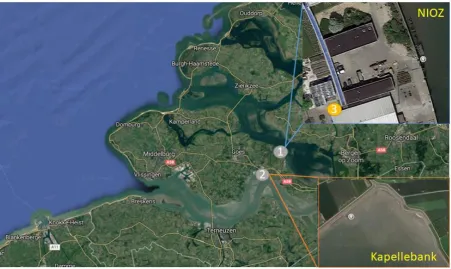
(18) The files from the ASED-sensor can be downloaded using a Wi-Fi connection. The file name of a certain ASED-sensor is 002-003A.SE2. Where 002 denotes the sensor-id, 003A is the measurement sequence number (in hex coding) and SE2 is the output format (Appendix A.1.4).. 2.2 Study sites 2.2.1 Lab experiments The travel time of the signal from the ASED-sensor to the bed and vice versa needs to be converted to a distance, to obtain a water depth. Therefore, analytic software needs to be developed. Before this can be done, lab experiments need to be collected to verify whether the ASED-sensor can measure the travel time in a range of environmental conditions. The lab experiments are measured under controlled environmental conditions. Thereafter the ASED-sensor will be used in the field. All lab experiments were obtained in a 300-litre water tank and in the wave flume at NIOZ. The water tank is placed outside, next to the greenhouse, at the NIOZ terrain in Yerseke (51°29’17” N; 004°03’26” E; Figure 2.5). Water from the Eastern Scheldt is used, which has an average salinity of 31.7 parts per thousand.. Figure 2.5: Location of the study sites. Location 1 is next to NIOZ which is in the Eastern Scheldt. Location 2 is the Kapellebank which is in the Western Scheldt. Location 3 is the greenhouse at the NIOZ terrain.. The wave flume of NIOZ (Figure 2.6) is used for testing the ASED-sensor during controlled waves and current forcing. The dimensions of the wave flume are 17 m long (2 m test section) x 0.6 m wide x 0.4 m deep (Figure 2.6). The current velocity can be changed from 0 to 80 cm/s and small regular waves can be made. The maximum wave height which can be created by the wave flume was 9.5 cm. The wave flume is filled with 30 cm of water from the Eastern Scheldt. First, the water from the Eastern Scheldt is saved in a big water tank and thereafter put in the wave flume. The same occurs when the water needs to be emptied from the wave flume. The big water tank is used to split the added chemicals from the water before the water is deposited in the Eastern Scheldt. The salinity in the wave flume is 31.2 parts per thousand.. Page 8 of 90.

(19) Figure 2.6: The wave flume of NIOZ (NIOZ website). Waves will propagate through the entire wave flume. At the end of the test section, the wave break material is placed under a gradient to damp the wave and reduce reflection (Figure 2.7). The experiment with current forcing does not have wave break material. Therefore, the current forcing could circulate through the entire wave flume. The set-up of the ASED-sensor for both waves and current forcing experiments is shown in Figure 2.8.. Figure 2.7: Wave break material for damping the waves. Figure 2.8: Set-up of the ASED-sensor for the waves and current measurements. 2.2.2 Field experiments The field experiments are performed in the Eastern Scheldt and in the Western Scheldt (Figure 2.5 location 1 and 2 resp.). Because the Eastern Scheldt was closed off from freshwater input from the Rhine, Meuse and Western Scheldt since 1969, the Eastern Scheldt formed a tidal bay (De Leeuw et al., 1992). Since then, the salinity remained nearly constant (De Leeuw et al., 1992). The tides are semidiurnal, with a tidal range of 4 m (data derived from Rijkswaterstaat (Ministry of Transport and Public Works)). The soil type of the Eastern Scheldt is sandy. The ASED-sensor is placed next to NIOZ (Yerseke) in a sand Page 9 of 90.

(20) soil type in the Eastern Scheldt (51°29’18” N; 004°03’29” E; Figure 2.5 location 1 resp.; Figure 2.9). The salinity is assumed to be 31.7 parts per thousand at the experiment location in the Eastern Scheldt.. Figure 2.9: Set-up of the field measurement in the Eastern Scheldt next to NIOZ. Figure 2.10: ASED-sensor. Western Scheldt experiment set-up. The Western Scheldt is a well-mixed estuary and is exposed to semidiurnal tides (Van den Berg et al., 1996; Horstman et al., 2011). Salinity at the mouth of the Western Scheldt (near Vlissingen ) is around 25 parts per thousand and around 10 parts per thousand at the Dutch-Belgian border, increasing during summer and decreasing during winter (Van Damme et al., 2005). The salinity is assumed to be 25 parts per thousand at the experiment location in the Western Scheldt (Figure 2.5 location 2 resp.; Figure 2.10). The tidal range in the Western Scheldt increases from approximately 4.2 m at the mouth (near Vlissingen) to 5.2 m at Hansweert (data derived from Rijkswaterstaat). The bed sediment of the Western Scheldt predominantly consists of well-sorted medium to fine grained sand (Van den Berg et al., 1996). The ASED-sensor is placed at the Kapellebank (51°27’35” N; 003°58’15” E; Figure 2.5 location 2 resp., Figure 2.10 and Figure 2.11). The soil type of the Kapellebank is for 88% silt and the median grain size (D50) is 16 𝜇m. The silty sediment of the Kapellebank can easily get in suspension. The SSC in the Western Scheldt has a high seasonal and tidal dependency (Fettweis et al., 1998). In the winter the SSC is 2 times larger than in the summer. This is explained by the freshwater discharge of the river. The tide average mud concentration is 1.3 to 1.7 times higher during a spring tide than during a neap tide (Fettweis et al., 1998). This encourages sediment deposition during the spring tide. If the ASED-sensor can measure the bed during these circumstances, the ASEDsensor should be applicable at all coasts, with a silty bed, as the Kapellebank.. Page 10 of 90.

(21) Figure 2.11: The field experiment in the Westerschelde at the Kapellebank. 2.3 Lab and field experiments 2.3.1 Lab experiments The lab experiments are conducted from 16th of October till 30th of October 2018. As mentioned above the ASED-sensor is evaluated during lab experiments in a water tank. The dimensions of the water tank (Figure 2.12.1) are a = 57.4 cm, b = 72 cm, c = 84 cm, d = 42 cm and e = 56 cm. The corners of the water tank give a strong reflection. Therefore, the ASED-sensor is not placed symmetrically in the water tank. The ASED-sensor is mounted using a steel ring whose inside is covered with rubber (Figure 2.12.3). With a bolt the ASED-sensor can be mounted on a wooden frame (Figure 2.12.3 and Figure 2.12.4).. 1. 2. 3. 4. Figure 2.12: ASED-sensor in lab set-up next to the greenhouse at the NIOZ terrain. Picture 1 is the front view of the lab set-up. Picture 2 is the tape measure with a metal plate. The clip surrounding the ASED-sensor can be seen in picture 3. Picture 4 is the top view of the lab experiment. The ASED-sensor is mounted on a wooden pole. The echologger is mounted on the yellow pole with on top the Global Positioning System (GPS) receiver.. Page 11 of 90.

(22) All the experiments are validated with manual measurements, by a tape measure. The tape measure has a metal plate at the end of the tape (Figure 2.12.2) and the benefit is that the metal plate did not disappear in the soft soil type. This improves the accuracy of the manual measurement up to 3 mm. For all the experiments the ASED-sensor will use a measurement frequency of approximately 300 kHz and, 8 individual measurements form a batch. Every individual measurement elapses 1 ms (=250ns * 4000) and the inter-measurement delay is 200 ms. The ASED-sensor has a short-term memory, which can be extended with SD-card. As the ASED-sensor measures, the measurements are first stored in the short-term memory and thereafter flushed to the SD-card. The short-term memory can only store 60 measurements, which are 7 full batches. As the measurements are sent in batches the flush from the short-term memory to the SD-card will be during the batches (60 measurements / 8 = 7.5). The ASED-sensor cannot store data during the data transfer from internal memory to external memory (SD-card). Therefore, immediately after a batch, the data is transferred from the short memory to the SD-card. This takes 1.3 seconds in time. Therefore, a measurement interval of 3 seconds between each batch is required. 2.3.1.1 Water depths First, the ASED-sensor is tested at different water depths. From this, the measurement domain can be obtained. A metal plate, which gives a strong reflection, covered half of the bottom of the water tank. The height of the ASED-sensor above the metal plate varies between 10 and 55 cm, with a distance interval of every 5 to 10 cm. The manual measurement was obtained by measuring from the metal plate to the waterline and from the waterline to the bottom of the ASED-sensor. The salinity is 31.7 parts per thousand during the experiments. 2.3.1.2 Soil types In tidal-flats different soil types occur, ranging from silt to mud to sand (Adam et al., 2006). Each soil type gives a different reflection of the acoustic signal. This depends on the absorption rate and the saturation rate of the soil type (Lurton, 2010). The different soil types will be put in a bucket below the ASED-sensor in the water tank (Figure 2.12.4). The bucket can carry 13 litres and the dimensions are width 21 cm x length 31 cm x height 19.4 cm. First, the soil was mixed well before putting the soil in the bucket. The bucket was filled with 10 cm soil and is covered with bubble plastic. Some seawater is put above the bubble plastic; therefore, the soil will not get in suspension in the water tank. The bubble plastic floated as the water in the water tank increased and the bubble plastic was removed. The measurements are done at depths of 20 and 40 cm. Six different soil types are used in this experiment. The first soil type is pure sand from the construction market. The second is silt obtained from Kapellebank (Western Scheldt) (Figure 2.5 location 2). Then, four different mixtures were made of these two soils. The idea is to add 20% silt to the sand and some salt water when needed to mix the new soil type. A 1.0 fraction of sand, 0.8 fraction of sand, 0.6 fraction of sand, 0.4 fraction of sand, 0.2 fraction of sand, and silt were expected. Because the obtained silt from the Westerschelde already had 0.12 fraction of sand in the soil, it was not possible to create these exact mixtures. Of each soil type, 3 samples were taken. The samples were freezedried in the laboratory, and the sediment distribution (Appendix A.2) of the soil was determined using a Malvern laser particle sizer. The eventually mixed results are 1.0,. Page 12 of 90.

(23) 0.80, 0.65, 0.48, 0.40 and 0.12 fraction of sand. A 0.80 fraction of sand means that the soil type contains 0.20 fraction of silt, which is defined as a grain size smaller than 63 𝜇m. 2.3.1.3 Dilutions of soil types When rough weather occurs, heavy wind and waves will get the upper layer of the bed in suspension. The sediment is mixed in the water. Therefore, it is necessary to know whether the ASED-sensor can measure the bed under these conditions. All soil types are used except 1.0 fraction of sand because it settles fast. Therefrom, the remained dilutions of the soil types were used. The dilutions are created by adding each time 20% water, so 80% soil and 20% water, 60% soil and 40% water and 40% soil and 60% water. The results of the different dilutions are tested at water depths of 0.20, 0.30 and 0.40 m (Table 2.1). The bucket with the dilutions of soil types was put in the water tank in the same way as described in 2.3.1.2. This experiment checks whether the ASED-sensor measures the upper layer of the dilution of the soil or it measures through the soil suspension and detects the bottom of the bucket. The manual measurement is obtained by first measuring the upper layer of the soil to the upper edge of the bucket (Figure 2.13 (1)). The tape measure continued from the bucket edge was measured to the waterline (Figure 2.13 (2)) and, from the waterline to the bottom of the ASED-sensor (Figure 2.13 (3)). Table 2.1: Dilutions (percentage water in the soil) of the soil types at measured depths of 0.20, 0.30 and 0.40 m. The values between the x and y-axis are the dilutions of the conducted experiments. Fraction sand in soil 0.20 m 0.30 m. 0.80. 0.65. 0.48. 0.40. 0.12. 16.37, 26.11 16.37, 26.11. 19.95, 20.00 19.95, 20.00. 0.40 m. 26.93, 45.47. 17.07, 18.12 17.07, 18.12 30.94, 43.86, 68.98, 90.37. 20.26, 21.75 20.26, 21.75 44.47, 52.42, 65.19. 57.50, 63.13, 72.45. 41.27, 52.45. Figure 2.13: Manual measurement from the soil to the transducer. Figure 2.14: Mixer powered by an electrical drilling machine. 2.3.1.4 Waves and current forcing The purpose of this experiment is to determine whether the ASED-sensor can measure the bed in the presence of waves. Therefore, the ASED-sensor is positioned 0.183 m above the bed of the wave flume, and increasingly larger waves were generated in the flume. The measurement started with no waves to check whether the ASED-sensor could measure. Page 13 of 90.

(24) the bed of the wave flume (Figure 2.8). Thereafter the waves started to increase every ten minutes by 1000 Rotations Per Minute (RPM). The RPM corresponds to a wave height (Table 2.2). The obtained experiments during waves are described in Table 2.2. Table 2.2: RPM versus wave height in the wave flume. flume setting in cm/s. velocity in cm/s. RPM. wave height in cm. 1000. 2. 200. 17. 1100. 3. 250. 23. 1200. 5. 300. 29. 1300. 7. 400. 38. 1400. 6.5. 500. 44. 600. 55. 700. 66. 1500. 9. 1600. 9.5. extra information. Table 2.3: Flume settings for the current of the wave flume. constant wave strong wave. During the current forcing experiment, the height of the ASED-sensor above the bottom of the wave flume was 0.227 m. The current started at flume setting 250 cm/s which corresponds to a velocity of 23 cm/s. The ASED-sensor measured the reflection of the signal by the bed in time (depth) the entire night. In the morning the current is set back to flume setting 200 cm/s. Every minute the flume setting increased by 100 cm/s until flume setting 700 cm/s. It takes 5 seconds to increase the current velocity. The flume settings can be translated into velocities in cm/s (Table 2.3). The flume was calibrated (Appendix A.3) before the experiment started.. 2.3.2 Field experiments The ASED-sensor is also tested in the field. Therefore, the ASED-sensor was first placed next to NIOZ (Yerseke) in the Eastern Scheldt during the weekend of 20 October 2018. The Eastern Scheldt has a sandy bed and therefore a strong reflection of the signal by the bed is expected. The Western Scheldt has very fine silt. The Western Scheldt data is collected in three weeks from the 1st of November till 23rd of November 2018. The idea was to measure for two weeks, to measure during a full tidal cycle (spring and neap tides). The ASED-sensor is mounted on a frame (Figure 2.9 and Figure 2.10). The long vertical pipes give the frame stability during wavy conditions. Another benefit of this frame is that scouring does not occur as it did with the predecessor the SED-sensor (Hu et al., 2015). Only point measurements at one location have been done, so only temporal variation can be observed. Each batch contains 8 measurements. The pressure sensor is enabled and set to a measurement interval of 5 Hz. Hereby, the waves are registered during the measurements in a submerged condition. For the determination of the inundation time, data from Rijkswaterstaat is used. 2.3.2.1 Eastern Scheldt The Eastern Scheldt is a tidal bay and sediment deposition occurs during rising tides. As flooding is the main mechanism for sediment delivery, the tidal flat is inevitably linked to sea level and tidal oscillations (Fagherazzi et al., 2012). Therefore, a lot of bed level dynamics occur, and it is interesting to observe this with the ASED-sensor. The length of the vertical pipes of the frame which enter the ground are 1.5 m long. This length is enough for a sandy bed. The ASED-sensor measured with a measurement interval of every 5 minutes and was set at a height of 39.0 cm above the bed (Figure 2.9).. Page 14 of 90.

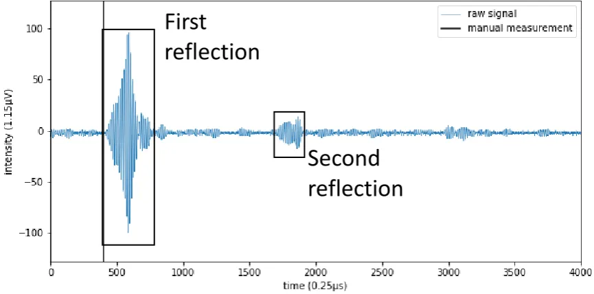
(25) 2.3.2.2 Western Scheldt The Western Scheldt is a tidal bay as well, but here the bed is very silty. Therefore, the length of the vertical pipes of the frame which enter the ground are now 2 m long. This length is necessary for stability in the silty bed. The ASED-sensor had a measurement interval of every minute. The measurement interval was chosen to check whether waves affect the deformation of the bed. The manual measurement was at the start of the experiment at a depth of 0.258 m and after three weeks 0.270 m. The bed eroded in the three weeks. Three erosion pins (Stokes et al., 2010; Gedan et al., 2011) are located 2 metres from the frame (Figure 2.15). Erosion pins are used to record the local surface level. The erosion pin is a very thin metal rod (i.e., to prevent scouring) with a height marker on top and a ring around the pin. The pin was pushed into the sediment, with the marker at a fixed height above the sediment. A metal ring was placed around the pin on top of the soil surface. The distance from the marker to the soil surface and the ring buried into the sediment were measured (Willemsen et al., 2018). The erosion pin showed an erosion of 0.009 m.. Figure 2.15: Three erosion pins (two erosion pins in the left red box) in the Western Scheldt experiment. 2.4 Converting raw data to bed levels Yet no analysing method existed at the start of this study. In the raw data of the ASEDsensor, a bed needs to be determined. As mentioned in paragraph 2.1, it is assumed when the amplitude suddenly increases, this denotes the reflection of the signal by the bed (Figure 2.16). Therefore, a method is required to find this sudden increase in amplitude. In general, the beginning of the signal has a lot of noise (Figure 2.16). As the ASED-sensor will be used in shallow water, multiple reflections of the bed level can occur. These reflections are reflected by the transition from water to air and by the bed. Figure 2.16 shows three reflections of the bed. In general, the first reflection has a higher intensity peak compared to the remained reflections and therefore the bed will be detected at the first strong reflection. The first strong reflection occurs around time step 600 (0.25 𝜇𝑠), so the distance between the ASED-sensor and the bed is approximately. Page 15 of 90.

(26) 1500𝑚⁄𝑠∗((613+600)∗0.25 𝜇𝑠) 2. = 0.227 𝑚. The other strong reflections occur around time step. 1800 (≈600+613+600) (0.25 𝜇s) and 3000 (≈1800+613+600) (0.25 𝜇s).. First reflection Third reflection Initial and periodic noise Second reflection. Figure 2.16: Raw data of the ASED-sensor above a metal plate. Multiple methods are tested to detect the first peak in the raw data so that it can be converted into bed levels. The chosen method must be applicable under various environmental conditions.. 2.4.1 Fast Fourier Transform As the ASED-sensor sends one signal into the water, multiple frequencies return. This can be due to multiple reflections, noise, etc. The Fast Fourier Transform (FFT) analysis is done to convert a signal into its corresponding frequency components, therefore the signal can be better analysed (Appendix A.5.1; Figure A.6.4). The frequency with the highest amplitude is the frequency which occurs the most in the data (Figure A.6.4). As the data is not infinite and no periodicity occurs, spectral leakage will appear. Spectral leakage can be minimized using windowing. The Hanning window will be used for the FFT analysis (Appendix A.5.1.1). This analysis is done with the real numbers of the FFT analysis. Before the FFT analysis can be done all negative values need to be removed; therefore, the absolute is taken of the raw data. The wavelength can be calculated using the frequency with the highest amplitude. The FFT analysis also provides an imaginary number and the phase of the returned signal can be determined. A depth value can be calculated by the combination of the wavelength and the phase of the returned signal (Figure 2.17; Table 2.4).. 2.4.2 Envelope method The sudden increase in amplitude can be found using the lower and upper envelope. The lower envelope are the minimum values of a line and the upper envelope are the maximum values of a line. The lower envelope is subtracted from the upper envelope, called delta envelope (Appendix A.5.2 Figure A.6.6). 1. Determine the sample with the maximum peak value; 2. Step back 300 (parameter) time steps; 3. From there determine the minimal value, going forward (i.e. towards the peak). Page 16 of 90.

(27) This will be the point used as the beginning of the reflection. To find this point, a few parameters can be set. The parameters which can be set are filtering initial and periodic noise (Figure 2.16, Figure 3.2 and Figure 3.3), strong reflections after the first reflection of the signal by the bed or a strong second part of the reflection (Figure 3.8), the point from which to start looking for the minimum. The bed detection range is 400 ≤ time step ≤ 2000. This corresponds to the assumed practical measurement domain of 0.20 m to 0.45 m. Mostly, the sudden increase in amplitude and the maximum intensity peak take a time of less than 300-time steps. Therefore, the sudden increase in amplitude will be found starting from 300-time steps backwards in time to the maximum intensity peak. As the start of the sudden increase in amplitude is mostly the minimum value before the maximum intensity peak. To find this start of the sudden increase in amplitude a n-value will be introduced. The n-value is a horizontal line to find the minimum value before the maximum intensity peak of the delta envelope line. The n-value starts from value 1.0 and increases 0.1 as the minimum value is not found. The intersection between the delta envelope line and the n-value line is until n-value 20. Mostly, a lot of noise occurs at a nvalue higher than 20, observed from the lab experiments. As the n-value intersects the delta envelope line that time step will be the bed detected depth in time. The bed detected depth in time needs to be converted into depth by. (𝑡𝑖𝑚𝑒 𝑠𝑡𝑒𝑝+613)∗250 𝑛𝑠∗𝑠𝑝𝑒𝑒𝑑 𝑜𝑓 𝑠𝑜𝑢𝑛𝑑 𝑚/𝑠 2. = bed. detected depth in metres. A median filter is applied for the bed detected depths of each batch, because it effectively removes impulsive outliers from the signal. As the bed is undetectable with the parameter settings, the values are not saved. These parameters are set as default settings (Figure 2.17). All parameters can be manually adjusted.. 2.4.3 Kalman filter The final analysed method evaluated was the Kalman filter. The Kalman filter is one of the most widely used methods for tracking and estimation due to its simplicity, optimality, tractability and robustness (Julier et al., 1997). The Kalman filter, rooted in the state‐ space formulation of linear dynamical systems, provides a recursive solution to the linear optimal filtering problem (Haykin, 2002). It applies to stationary as well as nonstationary environments. The solution is recursive in that each updated estimate of the state is computed from the previous estimate and the new input data, so only the previous estimate requires storage (Haykin, 2002). The raw data (Figure 2.16) is made positive by taking the absolute of the raw data (Appendix A.5.3.1). Most of the noise is removed by applying the Kalman filter. All parameters described in paragraph 2.4.2 are used in the Kalman filter method as well. Mostly, the maximum intensity peak of the Kalman filter line is above an intensity value of 10 (1.15 𝜇𝑉), observed from the lab experiments. This is an extra parameter addition to the envelope method. The Kalman filter, the window of the bed detection and parameters; the amount of time steps to find the minimum value from the maximum value and the nvalue, are set as default settings (Figure 2.17). All parameters can be manually adjusted.. Page 17 of 90.

(28) 2.4.4 All methods FFT method Preparing data. Absolute of raw data. Envelope method Delta envelope = upper – lower envelope of the raw data. Kalman filter Absolute of raw data. Kalman filter (weight 99% old and 1% new value). Smoothing. Windowing. Hanning windowing. Analysis. FFT analysis. Parameter settings. Real number for the wavelength. Bed level. Imaginary number for phase of the returned signal. Bed level. Find maximum peak 400 ≤ time step ≤ 2000. Find maximum peak 400 ≤ time step ≤ 2000. Look 300-time steps back from the maximum peak to find the minimum value. Look 300-time steps back from the maximum peak to find the minimum value. Using n-value to detect the bed level. Using n-value to detect the bed level. Applying median filter over each batch. Applying median filter over each batch. Bed level. Bed level. Figure 2.17: Flow chart of the converting methods. Page 18 of 90.

(29) To test the three methods, the experiment was done above a metal plate at a fixed depth. The manually measured depth is 0.284 m. The experiment has 2583 measurements. A burst of 8 measurements is analysed. First, the FFT method will be analysed. The difference between the first and the second measurement is 0.018 m (Table 2.4). This is due to the frequency fluctuations. The standard deviation of the FFT method is 0.008 m, for the envelope method 0.010 m and for the Kalman filter method 0.002 m (Table 2.4). The idea is that once a month the data is collected from the ASED-sensor. Therefore, another downside is the 5 minutes computation time of the envelopes of only 2583 measurements. The bed detection of the FFT yields 0.028 m deeper than the manual depth. The converting methods are applied by using scripts written in Python version 3.6. The envelope method and the Kalman filter method start increasing at the sudden increase in amplitude (Figure 2.18). As the ASED-sensor is placed above soil type 0.48 fraction of sand at a manually measured depth of 0.210 m. The delta envelope bed detection starts before the sudden increase in amplitude and therefore this method detects the bed at too shallow depths (Figure 2.19). The Kalman filter bed detection starts when a sudden increase in amplitude appears (Figure 2.19). The Kalman filter method will be used for analysing the bed detected depths and thus measuring sedimentation and erosion (Table 2.5).. Figure 2.18: Comparison of the delta envelope and Kalman filter method. The ASED-sensor measures above a metal plate at a manually measured depth of 0.284 m = 932 (0.25 𝜇s).. Page 19 of 90.

(30) Figure 2.19: Comparison of the delta envelope and Kalman filter method. The soil type of the bed is 0.48 fraction of sand.. Page 20 of 90.

(31) Table 2.4: All methods used to convert the raw data into bed levels. The first 8 single measurements (one batch) are observed. This measurement was applied above a metal plate at a depth of 0.284 m.. Single signal FFT FFT Envelope Kalman. freq [Hz] depth [m] depth [m] depth [m]. 1. 2. 3. 4. 5. 6. 7. 8. 325163 0.313 0.288 0.288. 314157 0.295 0.255 0.281. 325163 0.313 0.284 0.288. 314157 0.296 0.287 0.288. 314157 0.295 0.286 0.286. 325163 0.312 0.286 0.284. 325163 0.312 0.278 0.286. 325163 0.312 0.286 0.288. Average [m] 321036 0.306 0.281 0.286. Median [m] 325162.581 0.312 0.286 0.287. Stdev [m] 5328.016 0.008 0.010 0.002. Table 2.5: The advantages and disadvantages of the converting methods for the raw data into bed levels. Fast Fourier Transform 2 minutes Frequency fluctuates and therefore bed detected depth fluctuates. Envelope method 5 minutes. Kalman filter 40 seconds. High bed detected depth fluctuations. Bed detected depth fluctuates. Bed detected depth standard deviation. 0.008 m. 0.010 m. 0.002 m. Manual depth versus bed detected depth. The bed detected depth is 0.028 m deeper the manual measurement. The bed detected depth is 0.002 m deeper the manual measurement. The bed detected depth is 0.003 m deeper the manual measurement. Raw data reflection of the signal by the bed versus the bed detected depth. The bed is detected too deep compared to the reflection of the signal by the bed. The bed is detected too shallow compared to the reflection of the signal by the bed. The bed is detected exactly where the sudden increase in amplitude occurs in the reflection of the signal by the bed. Computation time Bed detected depth fluctuates. Page 21 of 90.

(32) 3 Results Firstly, the raw signal of the ASED-sensor will be explained during the submerged and non-submerged conditions. Secondly, the raw signal of the ASED-sensor during the lab and field experiment will be clarified. Thirdly, the converted raw data to bed level data will be analysed. Finally, the obtained theoretical and actual accuracy of the ASED-sensor is described.. 3.1 Measuring with the ASED-sensor 3.1.1 Being submerged or not Due to tides, the ASED-sensor is half of the time submerged during the field experiments. The difference between the non-submerged and submerged conditions can be clearly recognized in the raw data of the ASED-sensor (Figure 3.1). During non-submerged conditions, the initial part of the signal (approximately from t = 0 until t = 700) has a lot of noise and no bed is detected (blue line; Figure 3.1). A little initial noise occurs during submerged conditions (orange line; Figure 3.1). The submerged signal has a bed reflection with an intensity of around 100 (1.15 𝜇𝑉) time step 1600 (0.25 𝜇𝑠; orange line; Figure 3.1).. Figure 3.1: Non-submerged and submerged reflection of the raw signal of the ASED-sensor during the field experiment, Eastern Scheldt.. 3.1.2 The speed of sound in water The obtained time needs to be converted to depth values by multiplying by the speed of sound (c) to calculate the depth (d), see Equation 1. 𝑚 𝑐 [ ] ∗ 𝑡[𝑠] 𝑠 = 𝑑 [𝑚] 2. (1). Four speed of sound formulas, namely Del Grosso (Appendix A.6.1), Coppens (Appendix A.6.2), Mackenzie (Appendix A.6.3), and UNESCO – Chen and Millero (Appendix A.6.4) are compared with each other. By the calculation of the speed of sounds different salinities, depths or pressures and temperatures were used (Appendix A.6.5). The speed of sound in water will be calculated using the formula of UNESCO – Chen and Millero.. Page 22 of 90.

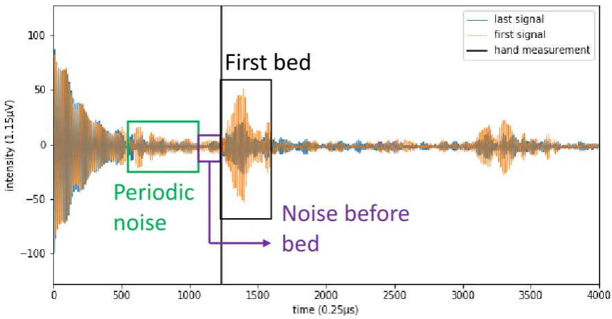
(33) 3.2 Collecting raw data 3.2.1 Lab experiments The ASED-sensor can detect the reflection of the signal by the metal plate as bed at a manually measured depth of 0.284 m (Figure 3.2). The ASED-sensor measured 295 bursts for 14.8 minutes during this experiment. The signal of the ASED-sensor does change over time, although the bed is fixed during the lab experiments. The first signal is the raw data collected by the first measurement of the experiment and the last signal is the raw data collected by the last measurement of the experiment. The first signal has less initial noise (approximately t = 0 until t = 700) than the last signal (Figure 3.2).. Initial noise. First bed reflection. Second bed reflection. Figure 3.2: The first and last signal of the raw data of the ASED-sensor. The ASED-sensor is placed above a metal plate at a manually measured water depth of 0.284 m = 931 (0.25 𝜇s).. This time the experiment lasts for 20 minutes and the manually measured depth is 0.340 m. Both signals have a lot of initial and periodic noise (Figure 3.3). The reflection of the signal by the bed has a higher intensity for the first signal and a lower intensity for the last signal (Figure 3.3). A combination of increasing initial noise and decreasing bed reflection intensity occurred over time. These circumstances can occur during all the experiments and therefore can possibly influence the conversion of the raw data into bed levels. The reflection of the signal by the bed occurs mostly deeper than or around the manual measurement. At depths before the manual measurement and the reflection of the signal by the bed mostly noise occurs (Figure 3.1, Figure 3.2 and Figure 3.3). The 4 mm lime/sealer is added to the manually measured depths.. Page 23 of 90.

(34) First bed reflection. Periodic noise. Noise before bed reflection. Figure 3.3: The first and last signal of the raw data of the ASED-sensor. The ASED-sensor is placed above a metal plate at a manually measured water depth of 0.340 m = 1230 (0.25 𝜇s).. 3.2.1.1 Water depths The ASED-sensor is tested at different depths measured above a metal plate at a manual depth of 0.115 m, 0.210 m, 0.284 m, 0.340 m, 0.395 m, 0.440 m, 0.497 m and 0.572 m (Table A.6.8). The speed of sound is 1475.3 m/s during the manual depth of 0.115 m (Figure 3.4). The bed should be visible at time step. 0.115 𝑚 𝑚 𝑠. 1475.3 ∗250 𝑛𝑠. ∗ 2 − 613 = 11. Initial noise occurs at that. time (Figure 3.4) and therefore the ASED-sensor is unable to detect the reflection of the signal by the bed. The second and the third reflection are easily detected at time step 700 and time step 1250 (Figure 3.4).. First reflection Third reflection. Second reflection Figure 3.4: The ASED-sensor is placed above a metal plate at a manually measured water depth of 0.115 m = 11 (0.25 𝜇s).. The raw signal of the ASED-sensor at a water depth of 0.210 m and 0.284 m (depths ≤ 0.30 m) changes over time like in Figure 3.2. The raw signal of the ASED-sensor at a Page 24 of 90.

(35) water depth of 0.340 m, 0.395 m, 0.440 m, 0.497 m and 0.572 m (depths > 0.30 m) changes over time like in Figure 3.3. The shallow depths ≤ 0.30 m (Figure 3.2) have a narrower reflection of the signal by the bed and the intensity of the signal reflected by the bed is 100 (1.15 𝜇V). The deeper depths > 0.30 m (Figure 3.3) have a wider reflection of the signal by the bed, have an intensity of the signal reflection by the bed of around 50 (1.15 𝜇V) and the last signal has a lower intensity peak compared to the first signal (Figure 3.3). The second reflection cannot be observed for water depths from 0.440 m, because the second reflection occurs after the registration time frame (after time 4000 (0.25 𝜇s); Table A.6.8). The intensity of the reflection of the signal by the bed is low at a manually measured depth of 0.497 m and 0.572 m (Table A.6.8). Therefore, the bed cannot be detected. 3.2.1.2 Soil types The bed reflection of 1.0 fraction of sand has a lot of initial noise at a manually measured depth of 0.186 m. The reflection of the signal by the bed cannot be detected (Table A.6.9). Soil type 0.8 fraction of sand has no initial and periodic noise and the reflection of the signal by the bed is easily detected (Figure 3.5; Table A.6.9). The second reflection by the bed is visible around time step 1800 (0.25 𝜇s) (Figure 3.5). The reflection of the last signal by the bed is shifted to the right (deeper) compared to the first signal for 0.40 fraction of sand (0.179 m). At a depth around 0.20 m 0.65, 0.48 and 0.12 fraction of sand have a clear bed detection and no to a little initial noise (Table A.6.9).. First reflection. Second reflection. Figure 3.5: Soil type 0.8 fraction of sand at a manually measured depth of 0.188 m = 404 (0.25 𝜇𝑠).. All soil types can detect the signal reflected by the bed at a manual measurement of around 0.40 m (Table A.6.9). Soil types 1.0, 0.65 and 0.48 fraction of sand of noise before the reflection of the signal by the bed and therefore are detected shallower than the manual depth. The shape of the signal reflected by the bed changes for varying depths and having the same soil type. The shape of the signal reflected by the bed changes as well for the varying soil types at a constant depth. There is no consistency in the shape of the signal reflected by the bed for the soil types and the water depths. The deeper depths of around 0.40 m have a wider signal reflection by the bed compared to the shallower depths of around 0.20 m.. Page 25 of 90.

(36) 3.2.1.3 Dilutions The ASED-sensor is tested for five different dilutions of soil types at a manually measured depth around 0.20, 0.30 and 0.40 m (Table 3.1). Unfortunately, some soil types were no longer in stock and these measurements could not take place. Table 3.1: Manually measured water depths in metres of the soil type dilutions during the ASED-sensor measurement Fraction sand in the soil % of water in the soil. % of water in the soil. % of water in the soil % of water in the soil % of water in the soil % of water in the soil. 0.80 16.37 0.219 0.303 26.11 0.212 0.307 26.93 0.393 45.47 0.384. 0.65 17.07 0.244 0.331 18.12 0.197 0.305 30.94 0.365 43.86 0.36 68.98 0.389 90.37 0.427. 0.48 19.95 0.192 0.309 20.00 0.179 0.295 41.27 0.368 52.45 0.361. 0.40 21.75 0.197 0.299 20.26 0.205 0.287 44.47 0.385 52.42 0.374 65.19 0.380. 0.12. 57.50 0.366 63.13 0.358 72.45 0.357. All dilutions of soil type 0.8 fraction of sand can detect a reflection of the signal by the bed, except dilution 26.11% (0.307 m; Table A.6.10). The reflection of the last signal has a lot of initial noise and is shifted to the right (deeper) for dilution 26.11% (0.307 m). The second reflection of the bed is well visible for dilutions 16.37% (0.219 m and 0.303 m) and 45.47% (0.384 m). The intensity of the second reflection for dilution 16.37% (0.303 m) is higher than the first reflection of the signal by the bed. But the intensity of the second reflection is for the last signal weaker than for the first signal. Dilutions 17.07% (0.244 m and 0.331 m), 18.12% (0.197 m and 0.305 m) and 30.94% (0.365 m) of soil type 0.65 fraction of sand can be detected by the reflection of the signal by the bed (Table A.6.11). Dilution 43.86% has a lot of noise before the reflection of the signal by the bed and therefore the reflection of the signal by the bed cannot be detected. The first signal has a stronger intensity reflection of the signal by the bed for dilutions 43.86%, 68.98% and 90.37% (Figure 3.6). The reflection of the signal by the bed of the last signal is shifted to the right compared to the first signal for dilution 68.98%. The reflection of the signal by the bed is detected later than the manual depth for dilution 90.37% (Figure 3.6). Dilutions 19.95% (0.192 m), 20.00% (0.179 m and 0.295 m) and 41.27% (0.368 m) of soil type 0.48 fraction of sand can detect a reflection of the signal by the bed (Table A.6.12). The periodic noise is weaker than the reflection of the signal by the bed for the first signal. But the periodic noise has a stronger intensity than the reflection of the signal by the bed for dilution 19.95% (0.309 m (Figure 3.7)). Therefore, the highest intensity peak will be detected earlier. The dilution of 52.45% has high intensities of periodic noise and therefore the reflection of the signal by the bed of is not easily detected.. Page 26 of 90.

(37) Figure 3.6: Soil type 0.65 fraction of sand with 90.37% water in the soil at a manually measured depth of 0.427 m = 1696 (0.25 𝜇𝑠).. Figure 3.7: Soil type 0.48 fraction of sand with 19.95% water in the soil at a manually measured depth of 0.309 m = 1068 (0.25 𝜇𝑠).. Dilutions 20.26% (0.205 m), 21.75% (0.197 m and 0.299 m) of soil type 0.4 fraction of sand can detect a reflection of the signal by the bed (Table A.6.13). The reflection of the signal by the bed is weak for dilution 20.26% (0.287 m) and 44.47% (0.385 m), therefore the reflection of the signal by the bed is not easily detected (Table A.6.13). Dilution 44.47%, 52.45% and 65.19% have high intensities of periodic noise and therefore it is not clearly visual which reflection of the signal is the bed reflection. Dilutions 57.5% (0.370 m), 63.13% (0.358 m) and 72.45% (0.357 m) of soil type 0.12 fraction of sand have initial and periodic noise and the reflection of the signal by the bed cannot be detected (Table A.6.14). There is no consistency in the shape of the signal reflected by the bed for the dilutions and the water depths.. Page 27 of 90.

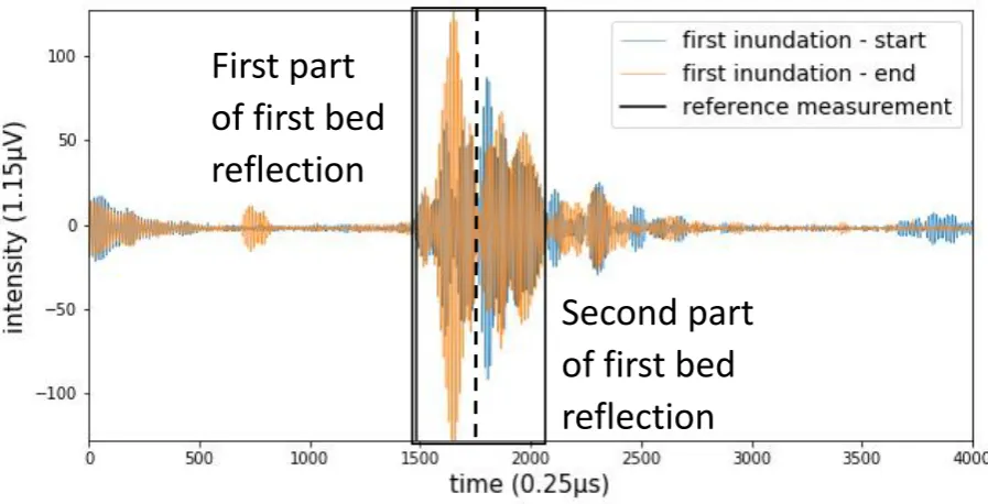
(38) 3.2.1.4 Waves and current forcing First, the ASED-sensor measured in waves forcing conditions. No initial and periodic noise occur before the reflection of the signal by the bed. The reflection of the signal by the bed is easily detected during waves. The length of the wave forcing experiment lasted for 62 minutes. Thereafter, the ASED-sensor measured in current forcing conditions. The length of the current forcing experiment lasted for 880 minutes = 14.7 hours. The raw data of the ASEDsensor has initial noise and low intensities of periodic noise. The reflection of the signal by the bed is easily detected. The intensity of the reflection of the signal by the bed is higher for the last signal than for the first signal. The shape of the signal reflected by the bed did not change significantly over time for the experiments during waves and current forcing. The practical measurement domain is from 0.20 m to 0.45 m, according to the raw data analysis of all lab experiments.. 3.2.2 Field experiments From 19th of October until 22nd of October 2018 the ASED-sensor was placed in the Eastern Scheldt (Figure 2.5). During that period, the ASED-sensor is five times inundated by the tide. Next, the ASED-sensor measured for 19 out of 23 days in the Western Scheldt (Figure 2.5). Because the battery dropped below 8 V. The ASED-sensor was inundated 37 times during this period. 3.2.2.1 Eastern Scheldt The raw data of all 5 inundations have been analysed. Starting with the first inundation, a little initial noise occurs (Figure 3.8). At the start of the first inundation, the shape of the reflection of the signal by the bed is different than for the middle and end of that first inundation. The reflection of the signal by the bed is split into 2 parts (Figure 3.8). The maximum intensity peak is higher in the second part of the first bed reflection for the start of the first inundation, this might influence the conversion of the raw data into bed levels. The middle and end of the first inundation have a higher maximum intensity peak in the first part of the first bed reflection (Figure 3.8). Therefore, the reflection of the signal by the bed can be detected at a deeper depth for the start of the first inundation than for the middle or end of the first inundation. At the end of the first inundation periodic noise occurs (Figure 3.8). The end of the first inundation has a higher intensity peak of the reflection of the signal by the bed than the start of the first inundation (Figure 3.8). The start of the reflection of the signal by the bed is clearly visual for the first inundation (Figure 3.8). The beginning of the reflection of the signal by the bed starts later for the second inundation compared to the first inundation, this could imply erosion. The shape of the reflection of the signal by the bed is like the middle and end of the first inundation. The intensity of the reflection of the signal by the bed is constant during the second inundation. The reflection of the signal by the bed is the same for the second, third and start of fourth inundation. But the shape of the signal changes from the third to the fourth inundation. The fourth inundation has several peak intensities like the start of the first inundation (Figure 3.8). The middle and end of the fourth inundation have noise before the reflection of the signal by the bed. Therefore, the bed will probably be detected shallower than the bed at the start of the fourth inundation. The shape of the reflection of the signal by the. Page 28 of 90.

(39) bed is the same for the fourth and fifth inundation. The fifth inundation does not have noise before the reflection of the signal by the bed. The maximum intensity peak of the raw signal moves to the right (deeper) during the last two inundations.. First part of first bed reflection. Second part of first bed reflection Figure 3.8: The start and end signal of the first inundation raw signal of the ASED-sensor in the Eastern Scheldt at a manually measured depth of 0.394 m = 1521 (0.25 𝜇𝑠).. 3.2.2.2 Western Scheldt Initial noise occurs for the first inundation (Figure 3.9). The start of the reflection of the signal by the bed is easily detected. The reflection of the signal by the bed changes in a three-week time scale. At the end, the reflection of the bed is still easily detected, but a second part of the signal reflected by the bed has a higher intensity for the start-middle of the first inundation (orange line; Figure 3.9), which happened as well during the Eastern Scheldt experiment (blue line; Figure 3.8). When the ASED-sensor is recently submerged, mostly the reflection of the bed has a high intensity (Figure 3.10) compared to the signal when it has been submerged for a while (Figure 3.9). As the ASED-sensor gets from a submerged to a non-submerged condition the last signal of the reflection of the bed is the same as when recently being submerged (Figure 3.10). A lot of noise occurs and the intensities of the entire signal increase during that moment. Therefore, it is better to leave the first and last signals out for the conversion of the raw data into bed levels. During the experiment, the reflection of the signal by the bed moves to the right (deeper). Therefore, erosion will be expected.. Page 29 of 90.

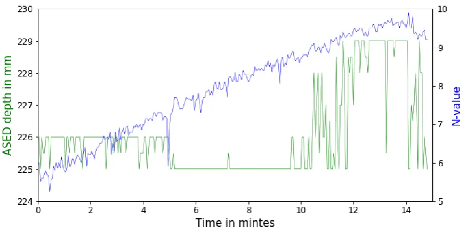
(40) Figure 3.9: The raw signal of start and middle start of the first inundation of the ASED-sensor in the Western Scheldt at a manually measured depth of 0.262 m = 823 (0.25 𝜇𝑠). (1632 vs 2168). Figure 3.10: A just submerged raw signal of the first inundation of the ASED-sensor in the Western Scheldt at a manually measured depth of 0.262 m = 823 (0.25 𝜇𝑠).. 3.3 Converting raw data to bed level data 3.3.1 Lab bed level All lab experiments with a clear visible reflection of the signal by the bed are converted to bed level data. The reflections of the signals by the bed that could not be detected are not converted to bed level data. 3.3.1.1 Water depths Each bed level is continuously measured for a period of about 15 minutes. The n-value increases over time for water depths 0.210 (Figure 3.11), 0.284 m and 0.440 m (Table 3.2). The n-value decreases over time for water depths 0.340 m and 0.395 m (Table 3.2).. Page 30 of 90.

(41) Manual depth 0.210 m - the bed detected depth is at 0.225 and 0.226 m for the first 10.4 minutes. Between 10.4 and 12.1 minutes, the bed detected depth is fluctuating between 0.225 m and 0.229 m. From 12.1 to 14.05 minute the bed detected depth is constant at 0.229 m and in the end, the bed detected depth fluctuates and ends at 0.225 m. Outliers occur between 0.225 and 0.229 m (Figure 3.11). The bed detected depth fluctuates during this measurement, while the bed is fixed.. Figure 3.11: ASED-sensor measured above a metal plate at a manually measured water depth of 0.210 m. The n-value and the ASED-sensor measured depth in mm over the length of time of the experiment.. Manual depth 0.284 - at the beginning the bed jumps between 0.285 m and 0.288 m and after 2.8 minutes the bed detected depth is constant at 0.286 m (Table 3.2). Manual depth 0.340 - at the beginning of the experiment, the reflected signal by the bed has a stronger intensity than the noise. After 45 seconds the noise has a stronger intensity than the reflected signal by the bed. Therefore, the bed cannot be detected with the default parameter settings and the parameter settings, need to be adjusted for searching the maximum intensity value from t=700 (0.25 𝜇s). Three depths are detected by the ASEDsensor around 0.327 m, 0.330 m and 0.343 m (Table 3.2). Manual depth 0.395 m - again, three depths are detected by the ASED sensor at 0.385 m, 0.386 m and 0.387 m (Table 3.2). Manual depth 0.440 m - the bed detected depth increased from 0.424 to 0.445 m for the first 9.4 minutes (Table 3.2). Thereafter the maximum intensity of the reflected bed was lower than the intensity of the noise at the beginning of the signal and therefore the parameter settings need to be adjusted for searching the maximum intensity value from t=500 (0.25 𝜇s).. Page 31 of 90.

No results found