warwick.ac.uk/lib-publications
A Thesis Submitted for the Degree of PhD at the University of Warwick
Permanent WRAP URL:
http://wrap.warwick.ac.uk/91571
Copyright and reuse:
This thesis is made available online and is protected by original copyright.
Please scroll down to view the document itself.
Please refer to the repository record for this item for information to help you to cite it.
Our policy information is available from the repository home page.
M A
O
D
C
S
Phase Field Models on Evolving Surfaces
by
David O’Connor
Thesis
Submitted for the degree of
Doctor of Philosophy
Mathematics Institute
The University of Warwick
Contents
Acknowledgments iv
Declarations v
Abstract vi
Chapter 1 Introduction 1
1.1 Overview . . . 1
1.1.1 The Phase Field Methodology . . . 1
1.1.2 The Method of Matched Asymptotic Expansions . . . 4
1.2 Outline of the Thesis . . . 6
Chapter 2 Calculus on Evolving Surfaces 8 2.1 Notation . . . 8
2.2 Some Important Identities . . . 10
2.3 Curves on evolving surfaces . . . 11
2.3.1 Notation . . . 11
2.3.2 Local Surface Reparameterisation . . . 13
Chapter 3 Asymptotics for the Evolving Surface Cahn-Hilliard Equa-tion 16 3.1 Introduction to the Cahn-Hilliard Equation . . . 16
3.1.1 Motivation of and remarks on the ESCH equation . . . 22
3.2 Assumptions for the asymptotic analysis . . . 23
3.2.1 Solution regime . . . 24
3.2.2 Outer expansions . . . 24
3.2.3 Inner coordinates . . . 24
3.2.4 Inner expansions . . . 26
3.3 Slow Mobility . . . 26
3.3.1 Outer solutions . . . 26
3.3.2 Inner solutions . . . 27
3.3.3 Discussion . . . 28
3.4 Fast mobility . . . 30
3.4.1 Asymptotic analysis . . . 30
3.4.2 Discussion . . . 33
3.5 The Deep Quench Limit . . . 34
3.5.1 Assumptions on the Solution Regime . . . 36
3.5.2 Asymptotic Analysis . . . 37
Chapter 4 Numerics 40 4.1 Overview . . . 40
4.2 The Surface Finite Element Method . . . 40
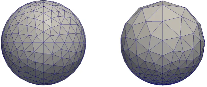
4.2.1 Approximation of Geometry and Triangulations . . . 40
4.2.2 Finite Element Spaces . . . 43
4.3 Function Spaces for Continuous Equations . . . 44
4.3.1 Weak Formulation . . . 45
4.3.2 Spatial Discretisation . . . 46
4.3.3 Time Discretisations . . . 48
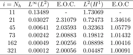
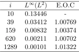
4.3.4 Convergence Tests . . . 49
4.3.5 Adaptive Refinements . . . 52
4.4 Numerical Experiments . . . 55
4.4.1 Stretching and Compression . . . 55
4.4.2 Bulk E↵ects . . . 58
4.4.3 A Solution on a Sphere with Tangential Mass Transport . . . 60
4.4.4 Scaling E↵ects . . . 62
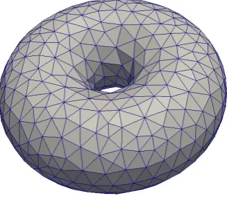
4.4.5 Topological Changes . . . 65
Chapter 5 Application: Cell Adhesion 68 5.1 Overview . . . 68
5.2 Introduction . . . 69
5.3 The Membrane Energy . . . 74
5.4 Model Derivation . . . 82
5.5 Asymptotic Analysis . . . 85
5.5.1 Assumptions . . . 85
5.5.4 Interface Coordinates . . . 91
5.5.5 Matching conditions . . . 92
5.5.6 Inner Solutions . . . 93
5.5.7 Remarks . . . 97
5.6 Simulating A Reduced Model . . . 100
5.6.1 Tangential Transport E↵ects . . . 105
5.6.2 Adhesion Patch Growth . . . 105
5.6.3 Changing Topology . . . 109
Chapter 6 Conclusion 115 6.1 Chapter 2 - Calculus on Evolving Surfaces . . . 115
6.2 Chapter 3 - Asymptotics for the Evolving Surface Cahn-Hilliard Equa-tion . . . 115
6.3 Chapter 4 - Numerical Simulations . . . 117
Acknowledgments
This work was supported by the UK Engineering and Physical Sciences Research Council (EPSRC) Grant EP/H023364/1 within the MASDOC Centre for Doctoral Training at the University of Warwick.
Thank you to my supervisor, Bj¨orn Stinner for all of his help and guidance throughout this project. Thank you, also, to everyone in MASDOC and Warwick who have made my time here a pleasure, especially my workmates Graham, Jorge and Ben.
Declarations
This thesis is submitted to the University of Warwick in support of my application for the degree of Doctor of Philosophy. It has been composed by myself and has not been submitted in any previous application for any degree. The work presented was carried out solely by the author, under the supervision of Bj¨orn Stinner.
Abstract
We study the asymptotic limit of some evolving surface partial di↵erential equations. We first examine the setting of an evolving surface with prescribed veloc-ity, extending the method of formally matched asymptotic expansions to account for the movement of the domain. We apply this method to the Cahn-Hilliard equation, considering various forms for the mobility and potential functions. In particular looking at di↵erent scalings of the mobility with respect to the interface thickness parameter. Mullins-Sekerka type problems are derived with additional terms which are due to the domain evolution.
We then consider the evolving surface finite element method and applying it to the Cahn-Hilliard equation in an evolving surface setting. We do this so as to support the theoretical findings as well as to further explore some interesting behaviour of solutions.
Chapter 1
Introduction
1.1
Overview
In Section 1.1.1 we introduce the notion of phase field models, discussing some of their history and appearances in the literature as well as motivating their uses. In Section 1.1.2 we introduce the method of matched asymptotics and explain its relation to the phase field methodology. We will give an account of some known works in the area. In Section 1.2 we give an outline of the structure of this thesis and highlight the novel results in each chapter.
1.1.1 The Phase Field Methodology
The phase field methodology is a powerful tool for simulating phase separation and interfacial evolution in a wide variety of applications. Partial di↵erential equations describing phase separation on evolving surfaces occur, for example, in de-alloying of binary alloys Eilks and Elliott [2008], in two-phase flow Hohenberg and Halperin [1977] (potentially with soluble surfactants H. Garcke and Stinner [2013]), in pattern formation on growing organisms Leung and Berzins [2003], or in phase separation on biomembranes Elliott and Stinner [2010b,a, 2013].
-1 0 1
x
-1 -0.8 -0.6 -0.4 -0.2 0 0.2 0.4 0.6 0.8 1
Phi(x)
Phase Field in PFM
-1 0 1
x
-1 -0.8 -0.6 -0.4 -0.2 0 0.2 0.4 0.6 0.8 1
Phi(x)
[image:10.595.224.410.115.267.2]Indicator Field in SIM
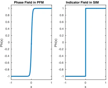
Figure 1.1: Comparison of sharp versus di↵use interface approach for a function which describes the regions. In the di↵use interface method changes continuously between equilibrium values rather than making a discontinuous jump. The interface in both exists atx= 0 with the interfacial region existing for|x|<0.1 in the di↵use interface approach.
described by the position of the interfacial boundaries. Usually a set of di↵erential equations is solved in each domain subject to flux conditions and constitutive laws at the interfaces.
In contrast, using the phase field technique, also known as a di↵use inter-face approach, a phase field variable is introduced to keep track of the boundaries between pure phases. Typically the phase field variable will take distinct values in the di↵erent phases with the phases now separated by a narrow region where the phase field variable transitions between the values associated to each phase. The sharp interface is then approximated as some level set of the phase field variable. See Figure 1.1 for a pictorial representation of the two settings.
di↵erential equations, possibly derived as a minimiser of some energy Elliott and Stinner [2013] or through a gradient flow dynamic involving the variation of an energy Cahn and Hilliard [1958]; Cahn [1961]. As early as 1893, van der Waals used the idea of continuous variations in density across an interface to model a liquid-gas system. In 1950 Landau and Ginzburg [1950], Ginzburg and Landau used a complex valued phase field variable to model superconductivity and in 1958 Cahn and Hilliard [1958] Cahn and Hilliard published their seminal paper utilising a thermodynamic formulation to account for the inclusion of gradients in thermodynamic properties. Phase field models need not be restricted to binary systems, with notable works by Steinbach et al. Steinbach et al. [1996]; Tiaden et al. [1998] and Garcke et al. Stinner et al. [2004]; Nestler et al. [2005] considering multiphase systems for arbitrary numbers of components. These multicomponent models naturally arise in the setting of material analysis, in particular in the solidification of alloys Cha et al. [2005].
Central to many phase field models is the use of the Ginzburg-Landau energy functional, which is an integral over the region under consideration of the following integrand:
( ,r ) := " 2|r |
2+1
"F( ), (1.1)
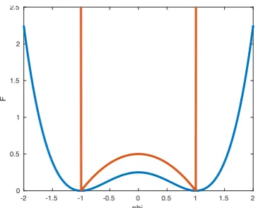
with the phase field variable,"the interfacial thickness parameter andF a poten-tial function. It has been used in the derivation of the Allen-Cahn equation Allen and Cahn [1979], the Cahn-Hilliard equation Cahn and Hilliard [1958] and for the modelling of two phase biomembranes Elliott and Stinner [2010a]. At the heart of this energy functional is the Landau term represented by the potential function,F. Di↵ering choices of potential function o↵er variations in the dynamics of each model. In many applications, F, is chosen to be of either double well type Elliott and Zheng [1986] or double obstacle type Blowey and Elliott [1991a]. As double well potential, it is standard to assume the formF( ) = 14(1 2)2, with this particular choice known as the standard double well potential. For a double obstacle type potential one might choose
F( ) = 1 2(1
2) +I
[ 1,1]( ) (1.2)
withI[ 1,1]( ) the indicator function of the interval [ 1,1] which takes value 0 when
is in the interval, and value 1 otherwise. Common to all potential functions are the minima, ua and ub, characterising the value of the phase field variable in
-2 -1.5 -1 -0.5 0 0.5 1 1.5 2
phi
0 0.5 1 1.5 2 2.5
[image:12.595.226.409.104.251.2]F
Figure 1.2: Two choices of potential. In blue the standard double well potential and in red the double obstacle type potential as in equation (1.2).
regions between the phase values.
The advantage of double-well type potentials are their smoothness properties but this is also their disadvantage since this can mean that the phase field variable does not always lie between the minima of the potential. In examples where a phase field model is used purely for interface tracking, Elliott and Stinner [2010a], this may not be a problem but in examples where the phase field variable has a physical interpretation, such as a density or concentration Eilks and Elliott [2008], it may not make sense for the phase variable to exceed it’s bulk values. The obvious difficulty of using a double-obstacle type potential is that the governing equations must be expressed in terms of variational inequalities and can be difficult to solve. In Elliott and Garcke [1996], the following logarithmic potential was considered:
F( ) = ✓
2[(1 + ) log(1 + ) + (1 + ) log(1 )] + 1 2(1
2) (1.3)
which has the advantage of being smooth but in the limit✓!0 tends to the double obstacle potential (1.2).
1.1.2 The Method of Matched Asymptotic Expansions
way the solutions of a free boundary problem. In some instances this is the case and the phase field model can be considered purely as an approximation of a free boundary problem. This limit of sending the interface width parameter to zero is known as an asymptotic limit or a sharp interface limit.
In the literature there are two types of asymptotic results on limits of phase field models. In works such as that of Pego Pego [1989] and Cahn et al. Cahn et al. [2006], the results are formal ones based on the method of formally matched asymptotics. The other type is of rigorous convergence as in the works of Bates et al. N. Alikakos and Chen [1994] or Le Le [2008]. In the former a rigorous justification was made of the asymptotics analysis and in the latter a Gamma-Convergence approach was used with an energy based argument, exploiting the gradient flow based structure of the model.
The method of matched asymptotics is formal in that it assumes the existence of a limiting free boundary problem. That is if "solves the di↵use interface problem, it is assumed that there is a sensible limit 0 in the sharp interface limit. The
question becomes then what problem should this sharp interface solution satisfy. By assuming a possible decomposition of the domain, asymptotic expansions are made in the interface width variable, for both the bulk or outer regions (areas is approximately constant) and the interfacial or inner regions (where rapidly transitions). It is an assumption of the method that these expansions exist. These two expansions are then assumed to agree in some intermediate region and sets of matching conditions can be derived.
The need for two di↵erent expansions is due to the rapid transitions of the phase field variable in the inner region. By considering a new set of co-ordinates and rescaling them appropriately with respect to", the interface is e↵ectively blown up to unitary width so that sensible limits of quantities dependent on " can be established.
The method of matched asymptotics has been carefully detailed in the work of Fife and Penrose Fife and Penrose [1995] and can also be found in Caginalp Caginalp [1989]. The method has been used for multi-component systems in Garke and Stinner [2006a] and has been extended to elliptic problems on stationary sur-faces Elliott and Stinner [2010a]. Much of the work in this thesis involves further extensions of the standard technique.
H 1 gradient flow of (1.1), or the Allen-Cahn equation Allen and Cahn [1979] which
is itsL2gradient flow, the convergence of the energy functional used in the gradient flow structure, in some appropriate manner, can be used to show convergence of solutions to the underlying gradient flows. The abstract framework can be found in the work of Serfaty Serfaty [2011].
It is known that the Ginzburg-Landau energy functional converges, in an appropriate sense, to the perimeter function i.e. the area function on the interface, and thus theL2 gradient flow of this functional results in mean curvature flow, and theH 1 gradient flow gives the Mullins-Serkerka flow.
1.2
Outline of the Thesis
We briefly describe the organisation of this thesis with a short summary of the contents of each chapter.
In Chapter 2 we define the common notation used throughout this work. In particular we discuss the notion of surface calculus, then introduce the framework for adding a time dependence to these surfaces and discuss some of the important identities that can be found in this area’s literature. There is also some discussion on useful results from di↵erential geometry that we employ to look at curves on evolving surfaces. The main result that we investigate in this chapter is the e↵ects of a time dependent surface on the change of variables formulae for use in our asymptotic analysis.
In Chapter 3 we consider a specific example of a phase field model on an evolving surface, namely the Evolving Surface Cahn-Hilliard (ESCH) equation. We use the results of the previous chapter alongside the method of matched asymptotic expansions to investigate the ESCH equations sharp interface limit. We consider general forms for its mobility and potential functions, initially restricting to smooth potentials, before looking at the case of a double obstacle potential. The novelty of this work comes from the postulation of an evolving surface and its e↵ects on the asymptotic analysis and limiting models
Chapter 2
Calculus on Evolving Surfaces
In this Chapter we discuss the elementary geometric analysis required throughout the remainder of this thesis. We first introduce the notation we have used in the context of surface calculus, introducing such structures as the surface gradient and the material derivative. We then look at how we can describe curves on evolving surfaces, introducing several di↵erent distance functions as well as the Darboux frame that we later use to reparameterise space locally around a given curve. Finally we present the result from O’Connor and Stinner [2016] with regards the change of variable formula for the signed distance function.
2.1
Notation
In this subsection we will discuss the notation and essential concepts of calculus on evolving surfaces required to describe partial di↵erential equations in moving and curved space. A more detailed introduction can be found in Dziuk and Elliott [2013] and Dziuk and Elliott [2007]. Since we have in mind physical systems we present the following under a setting of two-dimensional hypersurfaces evolving in a three dimensional ambient space. However some of the facts presented in this section can be generalised to other dimensions.
More specifically we consider a smooth, closed, compact and connected evolv-ing two-dimensional submanifold { (t)}t2[0,T] embedded in R3 for t 2 [0, T]. We
assume that it is orientable and denote by ⌫(·, t) : (t) ! R3,t 2 [0, T], a spatial
unit normal vector field. By (0) we denote the initial hypersurface. The space-time manifold for the moving surface is denoted by
GT :=
[
We have time-dependentmaterial surfaces in mind, thus a material particle plocated at xp(t)2 (t) at a timet2[0, T) has an associated velocityx˙p(t) which
determines the evolution of the shape. In addition we assume a smooth velocity fieldv(·, t) : (t)!R3,t2[0, T), such that x˙p(t) =v(xp(t), t).
For a function f : GT ! R the material derivative at a point (x, t) with
x2 (t) and t2(0, T) is defined by
@t•f(x, t) := d
dtf(xp(t), t) =
@f˜
@t(x, t) +v(x, t)·rf˜(x, t) (2.2) wherex=xp(t) for a material particlep located atx at time t. Note that for the
expressions on the right hand side to be well-defined a smooth extension ˜f of f to a neighbourhood ofGT is required however the value of @t•f is independent of this
extension Dziuk and Elliott [2013]. The normal time derivative@tf can be similarly defined by considering particle paths x⌫(t) that move in a direction normal to the
surface at all times. Thus ifx=x⌫(t) then
@tf(x, t) := d
dtf(x⌫(t), t) =
@f˜
@t(x, t) +v⌫(x, t)⌫(x, t)·rf˜(x, t) (2.3) wherev⌫ =v·⌫ is the normal component of the velocity. The normal time
deriva-tive represents time rate of change due to the normal motion of the surface and is related to the material derivative by the identity@t•f =@tf+v⌧·rf˜, withv⌧ the
tangential velocity. The tangential or surface gradient is defined as the projection of the standard derivative onto the tangent plane of the surface so that
r (t)f(x, t) :=rf˜(x, t) (rf˜(x, t)·⌫(x, t))⌫(x, t).
This quantity again makes use of any extension off to a neighbourhood of (t) and is also independent of this choice of extension. We denote byDi thei’th component of the surface gradient.
If w = (wi)3i=1,z = (zi)3i=1 : (t) ! R3 are smooth vector fields then r (t)wis the matrix with components (r (t)w)ij =Djwiand we write (r (t)w)T =
(Diwj)ijfor its transpose and use the scalar productr (t)w:r (t)z =Pi,jDjwiDjzi.
We will furthermore use the notationw⌦z for the matrix with entries wizj. The
surface divergence is defined by r (t)·w = tr (r (t)w) and the surface curl is defined with components r (t)⇥w i =✏ijkDjwk with✏the permutation tensor.
At any point x 2 (t) we define the projection P(x, t) := I ⌫(x, t)⌦
⌫(x, t) 2 R3⇥3, with I the identity matrix, to the tangent space T
x (t). Observe
r (t)w = rwP, r (t) ·w = P : r (t)w. The Laplace-Beltrami operator on
(t) is defined as the tangential divergence of the tangential gradient, (t)f = r (t)·r (t)f.
In contrast with the directional derivatives in planar space, the components of the gradient operator in curved space do not commute. For the commutation of derivatives we have the following result Dziuk and Elliott [2013]
DiDjf DjDif = r (t)⌫r (t)f j⌫i r (t)⌫r (t)f i⌫j. (2.4)
The symmetric matrixr (t)⌫ of the tangential derivatives of the normal field
is known as the Weingarten map or shape operator. And the mean curvature of (t) with respect to⌫ is defined as the negative of the trace of the Weingarten map:
m(x, t) = r (t)·⌫(x, t). (2.5)
We denote byg the Gaussian curvature. Withi the principle curvatures,i= 1,2,
it is the case thatm =1+2 and g=12. In addition we may write
g = 1
2(
2
m |r ⌫|2) (2.6)
with|r ⌫|2=r ⌫ :r ⌫. Furthermore, Elliott and Stinner [2010a]
⌫ = |r ⌫|2⌫ r m. (2.7)
2.2
Some Important Identities
For an arbitrary open subset V(t) ⇢ (t) and a function f(t) 2C1(V(t)) we have that Dziuk and Elliott [2013]
Z
V(t)r (t)
f =
Z
V(t)
fm⌫+
Z
@V(t)
fµext. (2.8)
Here,µext is the exterior co-normal on the boundary@V(t) that is tangent to (t),
pointing away fromV(t) and orthogonal to ⌫.
leaves and so pointsxmove with speedv(x, t), it reads Dziuk and Elliott [2007] d
dt
Z
V(t)
f =
Z
V(t)
@t•f+fr (t)·v. (2.9)
IfV(t)⇢ (t) is not a material volume and so material may enter or leave the region and thus the boundary moves with a speedv@V which may be di↵erent fromv, then
Betounes [1986] d dt
Z
V(t)
f =
Z
V(t)
@tf fmv⌫ +
Z
@V(t)
fv@V ·µext. (2.10)
Observe that the case (2.10) is a generalisation of (2.9). In the specific setting that v@V = v an integration by parts argument on the velocity terms shows that (2.9)
can be recovered. The time derivative of the Dirichlet inner product reads Dziuk and Elliott [2007]:
d dt
Z
(t)r (t)
f·r (t)g=
Z
(t)r (t)
f ·r (t)@t•g+r (t)@t•g·r (t)f (2.11)
+
Z
(t) r (t)·
vI 2D v r (t)f ·r (t)g
where D v := 12P r (t)v+r (t)vT P is the tangential deformation tensor or
symmetric gradient.
2.3
Curves on evolving surfaces
2.3.1 Notation
Let{⇤(t)}t2[0,T]denote a smooth, closed, and connected evolving curve on{ (t)}t2[0,T].
For all t2 [0, T] it splits the surface (t) into two domains which we denote b(t)
and a(t). Using the notion of the intrinsic distance between pointsx,y2 (t) (|·|2
being the standard Euclidean norm),
d (x,y, t) := inf
⇢Z 1
0 k
g0k2 g2C1([0,1], (t)), g(0) =x, g(1) =y ,
we can define the distance to the curve⇤(t) for a point x2 (t) as
d⇤(t)(x, t) := inf
and then thesigned distance function by
d(x, t) :=
8 < :
d⇤(t)(x, t) ifx2 b(t),
d⇤(t)(x, t) ifx2 a(t).
(2.13)
If we assume that⇤(t) and (t) are sufficiently smooth then there is a narrow tubular region of thickness ¯"> 0 (independent of t) such that for all points in this region there is a unique geodesic (modulo reparametrisation) which realises the distance. Define now the unit tangent vector along the geodesic by
µ(x, t) :=r (t)d(x, t), x2 (t)
which is a smooth function close to⇤(t) (by which we mean in the tubular region). Its derivative along the geodesic, (r (t)µ)µ = r (t)(r (t)d)µ, then is normal to (t). We now choose the unique ⌧(x, t) such that (⌧,µ,⌫) is a positively oriented orthonormal basis ofR3 on (t) close to⇤(t). Then
µ·(r (t)µ)µ= 0, ⌧·(r (t)µ)µ= 0. (2.14)
For the restrictions of⌧ and µto⇤(t) we will write
⌧⇤(x, t) :=⌧(x, t), µ⇤(x, t) :=µ(x, t), x2⇤(t).
Let now (s, t) :R⇤(t)S1⇥[0, T]!Rdenote a parametrisation of⇤(t) by arc-length. Here,R⇤(t)S1is the circle around the origin of radiusR⇤(t)which is such that
2⇡R⇤(t) is the length of⇤(t). Assume that the orientation of the parametrisation is such that s(s, t) =⌧( (s, t), t). Let us introduce
⌧ (s, t) :=⌧⇤( (s, t), t), µ (s, t) :=µ⇤( (s, t), t).
The curvature vector of ⇤(t) is given by ⇤(s, t) := @s⌧ (s, t) and, as ⌧ ·@s⌧ =
1
2@s|⌧ |2 = 0, can be decomposed up into a portion normal to (t) with coefficient ⌫ :=⇤(s, t)·⌫( (s, t), t). This coefficient is called thenormal curvature, similarly
we define the tangential coefficient
⇤( (s, t), t) =: (s, t) :=⇤(s, t)·µ (s, t) =@s⌧ (s, t)·µ (s, t) = ⌧ (s, t)·@sµ (s, t)
µ⇤
⌧⇤
µ
⌧
⇤(t)
d d
(s, t)
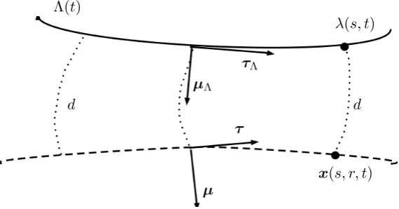
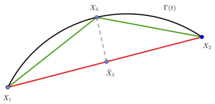
[image:21.595.164.449.60.209.2]x(s, r, t)
Figure 2.1: Sketch of geometric quantities describe in Section 2.3
2.3.2 Local Surface Reparameterisation
In Chapter 3 when employing the method of matched asymptotic expansions we will look to parametrise space locally around the interfacial curve so that we have a variable that scales with the interface width. We will then blow this variable up so that it scales independently from the interface width so that we can sensibly study the limit of fields in the sharp interface limit.
We may parametrise (t) close to⇤(t) asx (s, r, t) by extending the parametri-sation (s, t) wherex (s, r, t) is the solution of
˜
x(s,0, t) = (s, t), x˜r(s, r, t) =µ(x˜(s, r, t), t), r2[ ¯","¯].
For fixed sandt the curve r7!x (s, r, t) then is a geodesic and
d(x (s, r, t)) =r. (2.16)
Withv⇤(t) :⇤(t)!R3 we denote the (intrinsic) normal velocity of⇤(t), i.e.,
it can have a portion in direction⌫(t) and in directionµ⇤(t) butv⇤(x, t)·⌧⇤(x, t) = 0
for all x2⇤(t), t2[0, T]. Note that as ⇤(t)⇢ (t) for allt2[0, T] the velocity of ⇤(t) in the direction⌫(t) normal to the surface coincides with the one of the surface,
v⇤(x, t)·⌫(x, t) =v(x, t)·⌫(x, t) 8x2⇤(t).
However, the portion ofv⇤(t) which is tangential to (t) may be di↵erent from the
tangential portion ofv(t). Observe that
t(s, t)·µ (s, t) =v⇤( (s, t), t)·µ (s, t). (2.17)
of the surface gradient onto the curve⇤(t) then on ⇤(t) it holds that:
⌧·r (t)⌫⌧ =⌧·r⇤(t)⌫⌧ = ⌫·r⇤(t)⌧ ⌧ = ⌫·⇤ = ⌫ (2.18)
where we use that ⌫ ·⌧ = 0 for the interchange of derivative and have used that the surface gradient on⇤(t), given by r⇤(t) coincides with the derivative@s. This
gives us a method by which we may extend the normal curvature of ⇤(t) to the surrounding tube. Thus in the tubular region surrounding ⇤(t) we define ⌫ :=
⌧ ·r (t)⌫⌧. We also define the quantities
p:= µr (t)⌫µ, d:= ⌧ ·r (t)⌫µ(= µ·r (t)⌫⌧). (2.19)
Thus near the interface we can write the Weingarten map as
r (t)⌫ = ⌫⌧⌦⌧ pµ⌦µ d⌧⌦µ dµ⌦⌧. (2.20)
It can easily be shown that
m =⌫ +p, |r (t)⌫|2 =2⌫+2p+ 22d, g =⌫p 2d. (2.21)
Some other useful formulae are
@t⌫ = r (t)(v·⌫), @t•⌫ = (r (t)v)T⌫ (2.22)
@tm= (t)(v·⌫) +|r (t)⌫|2r (t)v·⌫ (2.23)
Using the reparameterisation of space x 7! (s, r) around a curve ⇤(t), we can rewrite a functionf : (t)!RasF :R⇤S1⇥[ ¯","¯]!R. Of importance later
on is the time rate of change of the signed distance function (2.13).
Let us consider a piont x 2 (t) with a distance of order " to ⇤(t) at a fixed time t, such that, without loss of generality, r(x, t) > 0. Let ˜t 7! xp(˜t) be
the path of a material point p such thatx = xp(t). For all ˜t close to t denote by
⇢7! gm(⇢,t˜) 2 (˜t) the geodesic which realises the distance d⇤(˜t)(xp(˜t)) defined in
(2.12), and denote byx⇤(˜t)2⇤(˜t) the initial point.
where the minus sign comes from the fact thatr(x, t)>0 so that µ⇤(x(t), t) is an
inward oriented unit tangential vector of the geodesic. The length of gm can also change by adding length at the end point. Analogously, this instantaneous change is given by
@txp(t)·µ(x, t) =v(x, t)·µ(x, t).
By the"closeness ofxto⇤(t) we can expand the last term inx⇤(t) and altogether
obtain
@t•r(x, t) = v(x⇤, t) v⇤(x⇤, t) ·µ⇤(x⇤, t) +O("). (2.24)
Observe that further contributions to the change of the length of the geodesic,gm,
Chapter 3
Asymptotics for the Evolving
Surface Cahn-Hilliard Equation
3.1
Introduction to the Cahn-Hilliard Equation
The subject of this chapter is the Evolving Surface Cahn-Hilliard (ESCH) equation
@t• + r (t)·v = r (t)·j, (3.1)
j= M( )r (t)w, w= " (t) +
1
"f( ). (3.2)
Here,{ (t)}t⇢Rn is a closed, smoothly evolving surface with a prescribed surface
velocity v : (t) ! R3, for material points of (t). The scalar function : (t)!
R is the phase field variable, " is the variable representing interfacial width, the function f( ) = F0( ) is the derivative of a double-well potential, and M( ) is a mobility function. The vectorj : (t)!Rnis the flux and w: (t)!R, known as
the chemical potential, is the variation of the Ginzburg-Landau energy
E"( (t)) =
Z
(t)
"
2|r (t) (t)|
2+1
"F( (t))dx (3.3)
and in the case v = 0 the system (3.1), (3.2) is the M( )-weighted H 1 gradient
flow of (3.3).
x
-1 -0.5 0 0.5 1
M(x)
[image:25.595.231.399.107.241.2]0 0.2 0.4 0.6 0.8 1
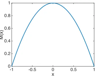
Figure 3.1: Example of a mobility function, Mdeg as defined in (3.6) with↵ = 1
and = 1.
F( b). Specifically, we have a quartic potential and a logarithmic potential in mind
defined by
Flog( ) = 2✓k1 (( ) log ( ) + ( ↵) log ( ↵))
✓c
2k2( )( ↵) (logarithmic), (3.4)
Fq( ) =
1
4( b )
2
( a)2 (quartic), (3.5)
where✓,✓c, k1, k2 >0 are parameters, but we stress that the results are not restricted
to these two cases. Qualitative examples of quartic type potentials can be seen in Figure 1.2.
We assume that the mobility M( ) is Lipschitz on [↵, ] and positive and continuously di↵erentiable on (↵, ) (the latter for simplicity, a slightly smaller open interval comprising [ a, b] would be sufficient). Qualitative examples can be seen
in Figure 3.1 We have in mind the two specific mobility functions:
Mdeg( ) =|M¯( ↵)( )| (degenerate), (3.6)
Mc( ) = ¯M (constant), (3.7)
where ¯M >0 is a constant. Let us introduce the pairings (Fq, Mc) and (Flog, Mdeg),
the former we refer to as theconstant mobility ESCH equation and the later as the
degenerate ESCH equation.
We refer to Novick-Cohen [2008] for a recent review of the equation. The field usually stands for the (mass or volume) concentration of one of the components, sometimes also their di↵erence. Cahn and Hilliard motivated the logarithmic double-well potential (3.4) in their original works Cahn and Hilliard [1958]; Cahn [1961] by theories of mixing. The parameter✓>0 is the (constant) temperature of the system and ✓c > 0 is a critical temperature dependent on the material which determines
the onset of phase separation. In the shallow quench limit (✓%✓c), the logarithmic
potential can be well approximated by the quartic potentials of the form (3.5). Non-constant mobilities were motivated by Cahn and Hilliard in the original derivation, see also Gurtin [1996]. But also the case of a constant mobility (3.7) has been of interest Elliott and Zheng [1986]; Bates and Fife [1993]; Novick-Cohen [1985]. In the limit ✓ ! 0 the logarithmic potentials converges to the double obstacle type potential
F1( ) = 1
2( )(↵ ) +I[↵, ]( ). (3.8) As mentioned in the introduction partial di↵erential equations describing phase separation on evolving surfaces occur in many examples. In contrast to the usual notion of the phase variable, , as a concentration, we here take an abstract point of view choosing not to physically interpret the phase variable. We only assume that is a conserved quantity for which (3.1) is a mass balance on the moving surface (t). In Section 3.1.1, we see how this assumption of mass conservation is used to derive the ESCH equation. By mass conservation we mean global mass conservation such that, R (t) (t) = R (0) (0) at all times t. This can be seen to hold by considering the weak form of (3.1) which reads
d dt
Z
(t)
⌘=
Z
(t)
M( )r (t)w·r (t)⌘ for all⌘ 2H1( (t)) a.e. t2[0, T].
Choosing as an admissible test function, ⌘ = 1, gives the result. The essential di↵erence to the standard Cahn-Hilliard equation is the r ·vterm in (3.1) which accounts for local stretching if r ·v >0 (or compressing in case of the opposite sign).
After the initial stage of separation, solutions to the Cahn-Hilliard equation exhibit large domains (or phases) in which is almost constant and close to one of the minima a, b of F. These phases are separated by moving layers with a
solution regime, by using formally matched asymptotics expansions, limiting free boundary problems (or sharp interface models) as " ! 0 have been derived. For the Cahn-Hilliard equation in a stationary, flat domain, the pairing (Fq, Mc) has
been considered by Pego [1989] whilst Cahn et al. [2006] have studied the pairing (Flog, Mdeg) including the deep quench limit ✓ & 0. The method has also been
applied to elliptic equations on fixed hypersurfaces in Elliott and Stinner [2010a] where also the underlying surface depends on the solution and, thus, on ". In some cases such expansions have been rigorously shown to converge, for instance, see Matthieu et al. [2008]; N. Alikakos and Chen [1994]. In N. Alikakos and Chen [1994] it is required that the resultant free boundary problem admits a smooth solution, thus imposing regularity assumptions on the initial condition. In Stoth [1996] these regularity assumptions are relaxed but with the restriction to radially symmetric solutions. Regarding other approaches to assess the sharp interface limit, the H 1-gradient flow (of the Ginzburg-Landau energy (3.3)) structure has been used in the context of -convergence to show asymptotic convergence to the Mullins-Sekerka problem in Le [2008] for the pairing (Fq, Mc). However, when working with
a deformable domain, without some relation coupling the surface velocity to the solution, the system does not necessarily have a gradient flow structure.
By considering the time derivative of (3.3) we see that d
dtE"( (t))
(2.11)
=
Z
(t)
"r (t) ·r (t)@t• "D vr (t) ·r (t) + "
2|r (t) |
2r
(t)·v
+
Z
(t)
1
"f( )@ •
t +
1
"F( )r (t)·v (2.8)
=
Z
(t)
" (t) @t• "D vr (t) ·r (t) + "
2|r (t) |
2r
(t)·v
+
Z
(t)
1
"f( )@ •
t +
1
"F( )r (t)·v (3.2)
=
Z
(t)
"w@t• "D vr (t) ·r (t) +"
2|r (t) |
2r
(t)·v
+
Z
(t)
1
"F( )r (t)·v (3.1)
=
Z
(t)
w r (t)·(M( )r (t)w) r (t)·v "D vr (t) ·r (t)
+
Z
(t)
"
2|r (t) |
2r
(t)·v+
1
(2.8)
=
Z
(t)
M( )|r (t)w|2
+
Z
(t)
✓
"
2|r (t) |
2+ 1
"F( ) w
◆
r (t)·v "D vr (t) ·r (t)
The first term is strictly dissipative, however it should be clear that examples can be constructed such that the term on the final line increases the energy. See for example the energy outputs in Section 4.4.3 or Section 4.4.5 for examples where the energy is increased due to the motion of the surface. Thus the potential for local compressing/stretching to increase the system energy means that the Cahn-Hilliard system does not posses a gradient flow structure unless some more assumptions are made on the velocity.
The general aim of this chapter is to investigate the impact of the motion of the underlying domain (t). Via a formal asymptotic analysis (for instance, see Fife and Penrose [1995]) we investigate the e↵ects of the surface motion on the limiting problem that is obtained as " ! 0. The methodology has been applied to surface phase field models in the stationary case where also the surface depends on " in Elliott and Stinner [2010a]. We have further extended the technique so that we can deal with moving surfaces and can apply it to the ESCH equation. As usual, a coordinate change using the signed distance function to the limiting moving phase interface is performed in the narrow interfacial region which blows up its thickness to unit length. But since the underlying space, (t), is time dependent, the scaled distance function must take account of transport due to the surface velocity. Technically, the challenge is to expand the material time derivative @t• in the new coordinates. The analysis is carried out for the case of hypersurfaces in the three-dimensional space (n= 3) but the ideas should carry through to the casen >3. The only difficulty should consist in dealing with several tangential coordinates along the limiting phase interface rather than one.
The scaling of M( ) (or rather ¯M) with respect to " turns out to be cru-cial when attempting to derive limiting free boundary problems. In the case of a stationary, flat domain (v = 0) it is equivalent to study the Cahn-Hilliard equation at di↵erent time scales as in Pego [1989]. Specific scalings have been considered in Novick-Cohen [2008] where ¯M ⇠"1 and Elliott and Ranner [2013] where ¯M ⇠"0. The former appears as a model for early time phase separation when the inter-faces form and the latter as a long time model for interface evolution. The scaling
¯
discussed in Caginalp [1989] in the context of a more general phase field model. We here consider a fixed time scale given by the evolution of the surface, namely one given by (a) a typical velocity at which the domains evolves and (b) a length scale given by the typical size of the surface. Di↵erent scalings of ¯M in "then relate to the speed at which di↵usion e↵ects are taking place in comparison with transport e↵ects.
Not for all scalings were we able to identify sensible limiting free boundary problems. If the mobility is too small, i.e., ¯M is of a high order in ", then the limiting problems do not see the long time behaviour resulting from the evolution of the phase field variable, whence the dynamics are purely governed by the transport with the given velocity field v. If the mobility is too high so that ¯M is of a low (negative) order in"then the asymptotic limits are forced towards equilibrium states with respect to the phases which are barely a↵ected by the transport.
In the interesting intermediate case in which ¯M is of order "0 we obtain the following evolving surface Mullins-Sekerka problem:
= i
r (t)· M( )r (t)w(t) = r (t)·v(t)
)
in i(t), i=a, b,
(3.9) [w(t)] = 0
w(t) = S⇤(t) 1
b a[M( )r (t)w(t)]·µ⇤(t) = v(t) v⇤(t) ·µ⇤(t)
9 > = >
;on ⇤(t). (3.10)
With, ⇤(t) the moving boundary separating the bulk phases b(t) and a(t), [·]
stands for the jump across⇤(t) when moving from a(t) to b(t),S >0 is a constant depending on the double-well potential F, ⇤(t) is the geodesic curvature of ⇤(t)
with respect to (t),v⇤(t) is the normal velocity of⇤(t), andµ⇤(t) is the co-normal
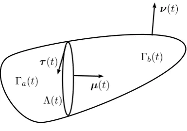
of⇤(t) with respect to (t) which points into b(t). A sketch of the physical setup described by this free boundary problem can be seen in Figure 3.2
a(t)
b(t)
⇤(t)
⌧(t)
µ(t)
[image:30.595.235.428.56.191.2]⌫(t)
Figure 3.2: Sketch of physical setting for Mullins-Sekerka type problems with im-portant quantities identified.
Ifr (t)·v= 0 then the procedure of Cahn et al. [2006] works however.
The remainder of this Chapter is set out as follows. We begin with a deriva-tion of the ESCH equaderiva-tion and some remarks on the e↵ects of rescaling the double-well potential. We then present our assumptions for performing an asymptotic analysis on an evolving surface. In particular we discuss the necessary expansion of the material derivative, @t•, in the inner co-ordinate system using the results from the previous chapter. Under the set up described we perform the asymptotic anal-ysis on the ESCH equation for the slow mobility, when ¯M ⇠"0, and interpret the results for specific mobility and potential functions. We then turn our attention to the fast mobility, when ¯M ⇠ " 1 and compare the result with the slow mobility. Finally we consider the deep quench limit ✓! 0 of the logarithmic potential (3.4) and analyse the resulting problem.
3.1.1 Motivation of and remarks on the ESCH equation
Following the lines of Elliott and Ranner [2013] we briefly derive the Cahn-Hilliard equation in the form (3.1), (3.2). Let (·, t) : (t) ! R,t 2 [0, T], be some scalar conserved quantity which means that for any test volumeV(t)⇢ (t) with external co-normalµext:
d dt
Z
V(t)
=
Z
@V(t)
j·µext (3.11)
with a flux j(·, t) : (t) ! Rm, t 2 [0, T] which is (spatially) tangential to (t).
Using (2.8) and the transport formula (2.9) yields
Z
V(t)
@t• + r ·v+r ·j= 0.
variation of the Ginzburg-Landau energy functional (3.3) so that
j = M( )r w.
Many results in the literature on the Cahn-Hilliard equation are obtained for a dimensionless version where the minima of the double well potential are located at±1. Our system can be transformed to such a setting as follows. Setting
˜ = b
b a
+ a
b a ,
= 12 (1 + ˜) b+ (1 ˜) a
to be the dimensionless form we define ˜F( ˜) := F( ) and ˜M( ˜) := M( ). Then f( ) =F0( ) = 2
b a
˜
F0( ˜) = 2
b a
˜
f( ˜), and a short calculation shows that (3.1), (3.2) takes the form
@t•˜ + ˜r ·v+c1r ·v = r ·
✓
˜
M( ˜)r w˜ c2 2
◆
(3.12)
˜
w = "c2 ˜ +
˜ f( ˜)
c2"
(3.13)
wherec1 = b+2 a,c2 = b2 a and ˜w is the chemical potential corresponding to the
first variation of the energy ˜E"( ˜) :=E"( ).
We remark that in Elliott and Ranner [2013] the case c1 = 0, c2 = 1 is
considered. The essential di↵erence is the source term proportional to the divergence of the surface velocity in (3.12).
Existence and uniqueness of the ESCH equation with constant mobility and standard double well potential was shown in Elliott and Ranner [2013] (in which the surface velocity was assumedC2, for a stationary planar setting with degenerate
mobilities and a double well type potentials in Elliott and Garcke [1996], and for constant mobilities and double obstacle type potentials in Blowey and Elliott [1991a].
3.2
Assumptions for the asymptotic analysis
techniques introduced in Section 2.3.2.
3.2.1 Solution regime
We consider solution regimes to (3.1)-(3.2) where phases have formed, in each of which is close to one of the two minima of F and which are separated by layers with a thickness that scales with". Let ( ", w")">0denote a family of such solutions
and assume that it converges to some pairing (u0, w0) such that, at each time t,
the spatial domain (t) is split up into domains a(t) ={
0(t) = a} and b(t) =
{ 0(t) = b}which are separated by a smooth, closed, and connected evolving curve
⇤(t) to which the level sets{ "(t) = ( b+ a)/2}converge. The asymptotic analysis
below, in principle, also works for several curves; however note that topological changes cannot be dealt with as they destroy the validity of the change of co-ordinates employed in the inner region. The aim is now to identify the equations that govern the evolution of⇤(t), 0(t), andw0(t).
3.2.2 Outer expansions
We assume that away from the interfacial layer around the curve⇤(t) we can expand the phase field variable and the chemical potential in the form
(x, t) =X
i
i(x, t)"i, w(x, t) =
X
i
wi(x, t)"i (3.14)
in each domain a,b(t).
3.2.3 Inner coordinates
As the thickness of the interfacial layer scales with"it makes sense to blow it up to unit length in order to be able to study the limit of fields and functions as"!0 in a meaningful way. We therefore introduce the scaled (geodesic) distance on (t) to the interface⇤(t) by
z:= r
". (3.15)
It is with respect to the new coordinates (s, z, t) we choose to work with in the interfacial layer. But before we state the (inner) expansions of the fields in these coordinates and state the matching conditions with the outer expansions in the adjacent domains we need to discuss how the di↵erential operators transform by the change of coordinates.
and Stinner [2010a]. For fixedtconsider the inversion of the mapR⇤(t)S1⇥[ ¯","¯]3
(s, r)!x (t)(s, r, t)2 (t) and letx2 (t) be a point with a distance to⇤(t) which
is O("). The identity (2.16) implies that "r (t)z(x, t) = r (t)r(x, t) = µ(x, t). Taylor expanding inx⇤:= (s, t) then yields
r (t)z(x, t) =
1
"µ⇤(x⇤, t) +r (t)µ(x⇤, t)µ⇤(x⇤, t)z(x, t) +O(").
Similarly we see that
r (t)s(x, t) =⌧⇤(x⇤, t) +O(").
For a scalar field : (t) ! R and a vector field : (t) ! R3 define (x, t) = (s, z, t) and (x, t) = (s, z, t) close to ⇤(t). Then we obtain for the surface gradient and the surface divergence in the new coordinates
r (t) (x, t) = s(s, z, t)r (t)s+ z(s, z, t)r (t)z
= 1" z(s, z, t)µ⇤(x⇤, t) (3.16a)
+ s(s, z, t)⌧⇤(x⇤, t) + z(s, z, t)r (t)µ(x⇤, t)µ⇤(x⇤, t)z+O("), r (t)· (x, t) = s(s, z, t)·r (t)s+ z(s, z, t)·r (t)z
= 1" z(s, z, t)·µ⇤(x⇤, t) (3.16b)
+ s(s, z, t)·⌧⇤(x⇤, t) + z(s, z, t)·r (t)µ(x⇤, t)µ⇤(x⇤, t)z+O(").
Using these identities, (2.14), and (2.15), a short calculation shows that we can write for the Laplace-Beltrami operator
(t) (x, t) =
1
"2 zz(s, z, t)
1
"⇤(x⇤, t) z(s, z, t) +O("
0). (3.17)
With regards to the operator@t• it will turn out that knowledge of the term to lowest order in"is sufficient for the asymptotic analysis. As
@t• (x, t) = s(s, z, t)@t•s(x, t) + z(s, z, t)@t•z(x, t)
and@t•z= 1"@•trwe need to focus on computing the leading order term of@•tr. Recall (2.24)
@t•r(x, t) = v(x⇤, t) v⇤(x⇤, t) ·µ⇤(x⇤, t) +O(")
so that
@t• (x, t) = 1
" z(s, z, t) v(x⇤, t) v⇤(x⇤, t) ·µ⇤(x⇤, t) +O("
3.2.4 Inner expansions
In conjunction with the outer region we will employ two "-expansions in the inner region. However, in contrast with the outer region, we will use the inner variables discussed in the previous section so that the expansions take the form
(x, t) = 1
X
i=0
i(s, z, t)"i, w(x, t) =
1
X
i=0
Wi(s, z, t)"i. (3.19)
The use of capitals is to distinguish between inner and outer variables.
3.2.5 Matching conditions
The above two expansions valid in the inner and outer regions should match in some intermediary region. Given an arbitrary outer field, , with expansion functions i
and i there are a set of matching conditions that these functions should satisfy.
These conditions are related to the spatial coordinates only and, thus, are indepen-dent of the movement of the domain. Therefore, and because a full derivation can be found in the literature (for instance, see Garke and Stinner [2006a]), we only state them here: In the limit asz!±1
0(s, z, t) ⇠ 0±(x⇤, t), (3.20a)
@z 0(s, z, t) ⇠ 0, (3.20b)
1(s, z, t) ⇠ 1±(x⇤, t)±r (t) 0±(x⇤, t)·µ⇤(x⇤, t)z, (3.20c) @z 1(s, z, t) ⇠ ±r (t) ±0(x⇤, t)·µ⇤(x⇤, t), (3.20d) @z 2(s, z, t) ⇠ ±r (t) ±1(x⇤, t)·µ⇤(x⇤, t) + µ⇤(x⇤, t)·r (t)
2 ±
0(x⇤(3.20e), t)z.
3.3
Slow Mobility
We begin identifying free boundary problems with the case ¯M ⇠ "0. As we will
briefly discuss below this is the highest scaling of the mobility in" (or the slowest mobility) for which a sensible free boundary problem occurs.
3.3.1 Outer solutions
Inserting the expansions (3.14) into (3.1) and (3.2), we match orders of". To order
" 1 (3.2) yields
which has 0 = a and 0 = b as stable stationary solutions. Motivated by the
assumptions on the setting at the beginning of Section 3.2.1 we can conclude that
0 = a in a and 0 = b in b which is the first equation of (3.9). To order "0
combining (3.1) with the flux term in (3.2) we obtain a bulk problem for the leading order term of the chemical potential:
0r ·v=r ·(M( 0)r w0). (3.22)
This is the PDE in (3.9). It remains to derive the interface conditions (3.10). For being able to apply the matching conditions we need to know whether 1is a suitable
field. So we briefly look at the equation to next order of (3.2) which reads
w0=f0( 0) 1.
3.3.2 Inner solutions
We now insert the expansions (3.19) into (3.1) and (3.2) and employ the change of variables formula (3.16). To the lowest order," 2, (3.1) yields
0 =@z(M( 0)@zW0). (3.23)
Thus there exists a function (s, t) such that M( 0)@zW0 = (s, t). Using the
matching condition (3.20b) and that M > 0 on ( a, b) we see that = 0 and
@zW0 = 0. This implies that w0 is continuous across the interface ⇤(t) in the
limiting problem which is the first condition of (3.10). To the order" 1 (3.2) yields
0 = @zz 0+f( 0). (3.24)
The matching condition (3.20a) implies that 0 ! a as z ! 1 and 0 ! b
asz! 1. The solution is the phase field profile. Well-posedness of the boundary value problem is discussed in Fife et al. [1979] and its references.
At the same order" 1 (3.1) gives thanks to the new expansion (3.18)
@z 0(v v⇤)·µ⇤+ 0@zv·µ⇤=@z(M( 0)@zW1). (3.25)
Here,v,v⇤,µ⇤, and@zv are evaluated at (x⇤, t) with the usualx⇤2⇤introduced
i.e., from 1 to +1, to obtain the last condition of (3.10),
( b a) v v⇤ ·µ⇤ = [M( 0)r w0]. (3.26)
Note that we have applied the matching conditions (3.20a) and (3.20d) to 0 and @zW1, respectively.
To the order"0 (3.2) gives thanks to (3.17)
W0= @zz 1 @z 0⇤+f0( 0) 1 (3.27)
where ⇤ is evaluated at (x⇤, t). We multiply by @z 0 and integrate over the
interfacial region. By di↵erentiating (3.24) with respect toz we see that @z 0 lies
in the kernel of the operator@zz f0( 0). Using this after an integration by parts
argument we obtain the following solvability condition:
w0 =S( 0)⇤ (3.28)
where
S( 0) =
⇣ Z
R(@z 0)
2⌘/(
b a)
is a constant depending on the phase profile of 0 and, thus, on the double-well
potential. This is the last condition of (3.10) so that we have derived the complete free boundary problem (3.9), (3.10).
3.3.3 Discussion
• Mass conservation: In the limiting problem (3.9), (3.10) the total mass is preserved (as it is in the ESCH equation):
d dt ⇣ Z b b + Z a a ⌘ (2.10) = Z b b
mv·⌫+
Z
⇤ b
v⇤·( µ⇤) +
Z
b a
mv·⌫+
Z
⇤ a
v⇤·µ⇤
(2.8)
=
Z
b br ·
v+
Z
⇤ b
(v⇤ v)·( µ⇤) +
Z
a ar ·
v+
Z
⇤ a
(v⇤ v)·µ⇤ (3.9)
=
Z
br ·
(M( b)r w) +
Z
ar ·
(M( a)r w) +
Z
⇤
( a b)(v⇤ v)·µ⇤
(2.8),(3.10)
=
Z
⇤
[M( )r w]·( µ⇤) +
Z
⇤
[M( )r w]·µ⇤ = 0. (3.29)
Thus, if b > a 0 there is a bound on the maximal and minimal surface
area where the bounds depend on the initial mass. This implies a restriction on the surface velocityv or the length of the time interval [0, T] for which the solution exists.
Observe that such a restriction also applies to the phase field model if the logarithmic potential (3.4) is used as then the value of is bounded from above by and from below by↵so that the total mass has to remain between
R
↵ and R . However, there is no such restriction in the case of a smooth, globally defined potential such as (3.5).
In turn, there is no restriction in either case, that is for the limiting free boundary problem nor the phase field model, if a<0< b.
• Constant mobility: For the case of a constant mobility and a smooth double-well potential such asFq, Pego [1989] has shown that the sharp interface limit
of the Cahn-Hilliard equation is the Mullins-Sekerka problem Mullins and Sek-erka [1963]. It corresponds to (3.9), (3.10) with a flat and stationary surface. One di↵erence is that the curvature, ⇤, now is thegeodesic curvature of the
interface. Another di↵erence is the addition of the transport term v ·µ⇤ in
the evolution law for the interface given in (3.26). The most important di↵ er-ence to the Mullins-Sekerka problem is the surface diverger-ence of the surface velocity in (3.22). In general, the chemical potential is no longer harmonic, and changes over time can occur due to the time dependence of the surface velocity.
of the chemical potential in the bulk can di↵er (see (3.22)) which also impacts on the jump term in (3.26). This result is independent of the choice of the double-well potential as long as the smoothness assumptions on (↵, ) are met and the minima are located at aand b. However, the choice ofF influences
the leading order profile (solution to (3.24)) and, thus, the values ofS( 0) in
(3.28). But by appropriate choice of coefficients such ask1 and k2 inFlog (or
a suitable prefactor forFq) one can ensure that S( 0) = 1.
• Slower mobility: Let us briefly consider the case of an even slower mobility ¯
M ⇠"1. Equation (3.21) still holds true while (3.1) yields to leading order that
0r ·v= 0. Within the solution regime defined in Section 3.2.1, which implies
that 0is constant in the bulk, we thus obtain the solvability conditionr ·v =
0. This is a strong restriction on the motion of the surface as it corresponds to local incompressibility. In (3.25) then W0 features instead of W1. With
the matching condition (3.20b) we then see that v⇤ ·µ⇤ = v ·µ⇤. So the
interface is simply transported with the surface velocity and any subtle front propogation due to the Cahn-Hilliard dynamics is lost. We remark that this is no contradiction to the results in Pego [1989] where, for the slow mobility, a Stefan type problem is shown to emerge because that limit is established at the next higher order in".
3.4
Fast mobility
A fast mobility scaling ¯M ⇠ " 1 has been used in Cahn et al. [2006] to derive surface di↵usion in the deep quench limit✓&0 of the Cahn-Hilliard equation with (Flog, Mdeg) on a flat and stationary domain. We will discuss this problem below
but first consider the general, non-degenerate case✓>0 or (Fq, Mc).
3.4.1 Asymptotic analysis
As previously we insert the expansions (3.14) and (3.19) into (3.1) and (3.2) and match orders of".
From the outer expansion of (3.2) to order" 1 we obtain again that
0= b
or 0 = a in b and a, respectively. Combining (3.1) with the flux term in (3.2)
we obtain to order" 1
Multiplying byw0 and integrating over b(t)[ a(t) we obtain using (2.8)
0 =
Z
b(t)
w0r · M( 0)r w0 +
Z
a(t)
w0r · M( 0)r w0 (3.31)
=
Z
b(t)
M( 0)|r w0|2
Z
a(t)
M( 0)|r w0|2
Z
⇤(t)
⇥
w0M( 0)r w0
⇤
·µ⇤.
To get an idea of what the jump term is we require information from the inner solutions.
The inner expansion of equation (3.2) yields the equation (3.24) to order" 1
and that 0 is again the phase transition profile. From (3.1) we obtain to order " 3 the equation (3.23) for W
0 again, and as before using the matching conditions
(3.20b) and (3.20a) we can conclude that
@zW0 = 0 and [w0] = 0. (3.32)
Using this and the orthogonality of µ⇤ and ⌧⇤, to order " 2 the same equation
yields
0 =@z M( 0)@zW1 .
Similarly, we can conclude that@zW1= 0 and, using the matching conditions
(3.20d) and (3.20c),
0 = [M( 0)r w0]·µ⇤ and [w1] = 0. (3.33)
Together with (3.32) we see that the last term of (3.31) vanishes, and we can con-clude thatr w0= 0 in b(t) and a(t) so that
w0(t) is constant on b(t)[ a(t). (3.34)
We have explicitly noted the time dependence to clarify thatw0 can and, in general,
will change over time (see below).
From equation (3.2) to order "0, which is (3.27) again, we can conclude as before that (3.28) holds true. With (3.34) we obtain that also
⇤(t) = 1
S( 0)
w0(t) is constant along ⇤(t) at all times t. (3.35)
Continuing with the outer expansions, (3.2) to order"0 yieldsw0 =f0( 0) 1
so that also 1is constant where we recall thatF00( 0) =f0( 0)6= 0 for 02{ a, b}
equation (3.1) to order"0 yields the following elliptic bulk problem forw
1:
0r ·v=r ·(M( 0)r w1). (3.36)
One boundary condition is given by (3.33). In order to determine a second one, consider the inner expansion of (3.1) to order " 1. Using (3.18) and that
@zW0 = 0,@sW0 = 0 (thanks to (3.34)), and@zW1 = 0 as well as the orthogonality
ofµ⇤ and ⌧⇤, a short calculation shows that it greatly simplifies to
@z 0(v v⇤)·µ⇤+ 0@zv·µ⇤=@z(M( 0)@zW2). (3.37)
It reads as (3.26) except that W1 is replaced by W2. Integrating with respect to
z over R, treating the left hand side in the same manner as done for (3.26), and applying (3.20e) to the right hand side where we use thatr w0 = 0 we arrive at
( b a) v v⇤ ·µ⇤ = [M( 0)r w1]. (3.38)
Returning to the higher order inner expansions, from equation (3.2) to order
"0, we obtain (3.27) again, and conclude as before that (3.28) holds true. With (3.34) we obtain that also
⇤(t) =
1 S( 0)
w0(t) is constant along ⇤(t) at all times t. (3.39)
SinceW0 =S( 0)⇤, writing 1= ˜⇤and substituting into (3.27), then ˜ can be
determined as the unique function solving
@zz˜ +f0( 0) ˜ =S( 0) +@z 0 (3.40)
subject to the boundary condition limz!±1@z˜ = 0 from (3.20b).
Finally at order"we obtain
W1 = @zz 2+@z 1⇤+f0( 0) 2+f00( 0) 2 1
2 (3.41)
This gives us a method to determine the interface condition for the first order term of the chemical potential. Multiplying by @z 0 and integrating as before we can
determinew1 to be:
w1 =
2 Z 1
@z˜@z 0
˜2
We may express this in a short from as
w1 =T( 0)2⇤,
whereT( 0) is a constant depending on the leading order phase profile in the inner
region. We have suppressed the dependence on ˜ by noting the dependence of ˜ on the phase profile 0 (see (3.40)).
3.4.2 Discussion
To summarise the findings of the preceding section: The phase interface is in spatial equilibrium in the sense that the geodesic curvature is constant, see (3.39). In the thus split domain we have the set of equations:
= i
r ·(M( )r w˜(t)) = r ·v(t)
)
in i(t), i=a, b,
(3.42) [ ˜w(t)] = 0
˜
w(t) =T(t)2⇤ 1
b a[M( )r w˜(t)]·µ⇤(t) = v(t) v⇤(t) ·µ⇤(t)
9 > = >
;on ⇤(t). (3.43)
• Restrictions due to compatibility condition: From (3.35) we have a compatibility condition that the curvature should remain constant, in addition we assumed a general surface evolution so thatv was arbitrary. However, this causes a problem as a general arbitrary velocity could drive the interface in di↵erent ways along its length so as to alter the geodesic curvature. Thus for a solution of the free boundary problem, in the fast mobility regime, to exist we cannot assume an arbitrary surface velocity but must instead assume that the evolution is such that the (spatially) constant curvature persists. This compatibility condition is thus rather restrictive.
• Mass conservation: First, observe that the total mass is still preserved in the sharp interface limit potentially implying a restrictions on the velocityv. In the identity (3.29)w has to be replaced by ˜w for this purpose.
much about the evolution of ⇤(t). In fact, at a given time t there may be several possible curves⇤(t) of constant geodesic curvature such that the mass side condition is satisfied. For instance, if (t) is a sphere one will find an infinite number. By the assumptions in Section 3.2.1 the interface is approx-imated by level sets of the phase field solutions. Thus, one may expect it to evolve smoothly, and one will also expect that a specific curve is picked in the sharp interface limit. We leave this question open for future studies.
3.5
The Deep Quench Limit
The deep quench limit of (3.1) and (3.2) for the degenerate ESCH equation corre-sponds to the limit as ✓ & 0. Then a ! ↵ and b ! so that the degenerate
mobilityMdeg( ) is switched o↵in the bulk. In the case of a stationary, flat domain
the limiting problem is surface di↵usion and has been derived in Cahn et al. [2006]. There, the flux j is expanded in addition to the fields and some matching condi-tions are replaced by assumpcondi-tions on the limits of the fluxes when approaching the boundaries of the interfacial layer. This is due to a lack of equations for the bulk fields.
Indeed, also in our case, (3.30) does not exist so that we have no equation for w0
in the bulk. In particular, we cannot conclude any more thatr w0 = 0. Similarly,
there is no bulk equation for w1: Equation (3.36) reduces to 0r ·v = 0. Within
the solution regime defined in Section 3.2.1 this means necessarily that
r (t)·v(t) = 0
in the bulk phases, the implication of which has been discussed in the context of a very slow mobility already (see Section 3.3.3). As we also cannot conclude any more that @sW0 = 0 another term of the form M(u0)@ssW0 appears on the right hand
side of (3.37). Integrating and using suitable assumptions for the fluxM( 0)@zW2
as in Cahn et al. [2006] we obtain
( b a) v(t) v⇤(t) ·µ⇤(t) = ˜S( 0) ⇤(t)⇤(t) (3.44)
instead of (3.38). Here, ⇤(t) corresponds to@ss after parametrisation and stands
for the Laplace-Beltrami operator on the curve⇤(t), and ˜S( 0) =S( 0)
R
RM( 0).
of the deep quench limit problem in an appropriate setting. In this section we will look to alter the asymptotic analysis to derive surface di↵usion more rigorously. Since we have in mind recovering something akin to (3.44), and bearing in mind the compatibility condition resulting from (3.36) we will consider a di↵erent system that we will call the non-conservative evolving surface Cahn-Hilliard equation (NESCH). Note that this is not a limit of our previous form for the ESCH. The non-conservative ESCH equation replaces (3.1) with the following
@t• =r (t)· M( )r (t)w . (3.45) The dropping of the term r (t)·v from (3.1) results in a relaxation of the
conservation assumption with regards the phase field variable, inspiring our naming it the non-conservative ESCH equation. Observe that in weak form (3.45) reads:
d dt
Z
(t)
⌘=
Z
(t)
⌘r (t)·v M( )r (t)wr (t)⌘ for all⌘ 2H1( (t)) a.e. t2[0, T]. (3.46) Upon testing with the admissible test function⌘= 1 we obtain
d dt
Z
(t)
=
Z
(t) r (t)·
v. (3.47)
In the case of local incompressibility,r (t)·v = 0, we obtain mass conservation again, however in the case of a non-divergence free velocity the total mass can change. Although we take the point of view of referring to the nESCH as a non-conservative form of the ESCH, a possible alternative interpretation is that conservation still holds, but that there is balancing of mass supply by adding the term r (t)·v to
the right hand side of (3.1) so that mass is added to the system at exactly the rate with which it would appear to be lost due to local stretching/compression.
Since we wish to study the deep quench limit of the logarithmic potential, (3.4), we consider the double obstacle type potential, (3.8). Since this is not di↵ er-entiable (3.2) must be expressed in the following form:
w+" (t) +
1
"(
+↵
2 )2@I[↵, ]( ). (3.48) In (3.48),@I[↵, ](·) is the subdi↵erential of the indicator function I[↵, ] for the in-terval [↵, ].