High fidelity sky models

warwick.ac.uk/lib-publications

A Thesis Submitted for the Degree of PhD at the University of Warwick

Permanent WRAP URL:

http://wrap.warwick.ac.uk/89934

Copyright and reuse:

This thesis is made available online and is protected by original copyright.

Please scroll down to view the document itself.

Please refer to the repository record for this item for information to help you to cite it.

Our policy information is available from the repository home page.

High Fidelity Sky Models

by

Pınar Satılmı¸s

Thesis

Submitted to the University of Warwick for the degree of

PhD in Engineering

Supervisors:

Prof. A. Chalmers, Dr K. Debattista

Warwick Manufacturing Group

Contents

List of Tables v

List of Figures vi

Acknowledgments ix

Abstract x

Chapter 1 Introduction 1

1.1 Motivation . . . 1

1.2 Approach . . . 3

1.3 Thesis Outline . . . 4

Chapter 2 Background 5 2.1 Light . . . 5

2.1.1 Radiometry . . . 5

2.1.2 Surface Interaction . . . 7

2.1.3 Light Sources . . . 10

2.2 Light Transport . . . 11

2.2.1 The Rendering Equation . . . 11

2.2.2 The Radiative Transfer Equation . . . 13

2.3 Monte Carlo Methods . . . 16

2.3.1 Stratified Sampling . . . 18

2.3.2 Importance Sampling . . . 18

2.3.3 Multiple Importance Sampling . . . 19

2.3.4 Other Methods . . . 19

2.4 Physically Based Rendering . . . 20

2.4.1 Rasterization . . . 20

2.4.2 Ray tracing . . . 20

2.4.3 Path Tracing . . . 21

2.4.4 Light Tracing . . . 22

2.4.6 Metropolis Light Transport . . . 23

2.4.7 Photon Mapping . . . 24

2.4.8 Progressive Photon Mapping . . . 25

2.4.9 Irradiance Caching . . . 25

2.4.10 Instant Radiosity . . . 26

2.4.11 Vertex Connection and Merging . . . 26

2.5 Rendering of Participating Media . . . 27

2.5.1 Monte Carlo Approach to Volumetric Path Tracing . . . 27

2.5.2 Volumetric Photon Mapping . . . 30

2.5.3 Radiance Caching for Participating Media . . . 31

2.5.4 Combined Estimators . . . 32

2.6 Machine Learning . . . 32

2.6.1 Supervised Learning . . . 32

2.6.2 Unsupervised Learning . . . 37

2.7 Summary . . . 38

Chapter 3 Skylight Modelling 40 3.1 Rayleigh Scattering . . . 41

3.2 Mie Scattering . . . 42

3.3 Henyey-Greenstein Phase Function . . . 45

3.4 Analytic Skylight Models . . . 45

3.4.1 Preetham Sky Model . . . 48

3.4.2 Hošek Sky Model . . . 49

3.5 Image-Based Lighting . . . 50

3.6 Clouds . . . 51

3.6.1 Properties of Clouds . . . 52

3.7 Cloud Modelling . . . 55

3.8 Cloud Classification . . . 58

3.9 Summary . . . 62

Chapter 4 Discussion & Methodology 63 4.1 Discussion on Skylight Modelling . . . 63

4.1.1 Skylight Modelling . . . 63

4.1.2 Cloud Classification Techniques . . . 64

4.1.3 Cloud Modelling and Rendering . . . 68

4.2 Research Question . . . 71

4.3 Objectives . . . 73

4.4 Methodology . . . 73

5.1 Modeling Skies with Neural Networks . . . 77

5.1.1 Sky Illumination Model . . . 77

5.1.2 Neural Network Representation . . . 78

5.1.3 Training . . . 82

5.1.4 Implementation . . . 83

5.2 Results . . . 84

5.2.1 RMSE Results . . . 84

5.2.2 Comparative Results . . . 85

5.2.3 Timings . . . 86

5.2.4 Discussion . . . 87

5.3 Summary . . . 88

Chapter 6 Physically-Based Cloud Modelling 89 6.1 Challenges in Reconstruction of Clouds . . . 90

6.2 Proposed Solution . . . 90

6.3 Characteristics of Proposed Method . . . 92

Chapter 7 Classification of Clouds from whole Sky HDR Images 93 7.1 Overview of the Classification Method . . . 94

7.2 Dataset . . . 96

7.3 Feature Vector Extraction based on the Patches . . . 96

7.4 Representative Feature Vector . . . 98

7.4.1 k-Means Clustering of Features . . . 99

7.4.2 Representative Cloud Type of the Clusters . . . 100

7.5 Classification of an HDR Image . . . 100

7.6 Results . . . 103

7.7 Discussion . . . 106

7.8 Conclusion . . . 108

Chapter 8 Modelling of Clouds from a Single HDR Image 110 8.1 Overview . . . 111

8.2 Theory . . . 112

8.3 Practical Solution . . . 114

8.3.1 Light Transport . . . 114

8.3.2 Optical Properties . . . 115

8.3.3 Spatial Properties . . . 116

8.3.4 Cloud Representation . . . 116

8.3.5 Initialisation . . . 118

8.3.6 Optimisation . . . 118

8.4.1 Lighting . . . 121

8.4.2 Rendering . . . 122

8.5 Results . . . 123

8.5.1 RMSE Results . . . 124

8.5.2 Comparative Results . . . 125

8.6 Discussion and Limitations . . . 125

8.7 Summary . . . 126

Chapter 9 Conclusion 134 9.1 A Machine Learning Driven Sky Model . . . 134

9.2 Physically-Based Cloud Modelling . . . 135

9.2.1 Cloud Classification . . . 135

9.2.2 Cloud Modelling . . . 135

9.3 Contributions . . . 136

9.4 Future Work . . . 137

List of Tables

4.1 References for the models in the Section 3.8. . . 66

4.2 Comparison of cloud classification techniques. . . 66

4.3 References for the models in the Section 3.7 . . . 69

4.4 Comparison of cloud modelling techniques. . . 69

5.1 Cross validation results for the trained sky models, time in seconds required to train the neural network and the number of examples. . . 84

5.2 Cross validation results for irradiance values generated by trained sky models. . 85

7.1 Symbols used in the chapter . . . 95

7.2 Interpretation of the cross validation results with a Confusion Matrix . . . 103

7.3 References for the models in the Section 3.8. . . 109

7.4 Comparison of cloud classification techniques. . . 109

8.1 The absorption and scattering coefficients for water and ice clouds used in the method. . . 124

8.2 Cross validation results of RMSE calculations. . . 125

8.3 Cross validation results for irradiance values. . . 125

8.4 References for the models in the Section 3.7. . . 133

List of Figures

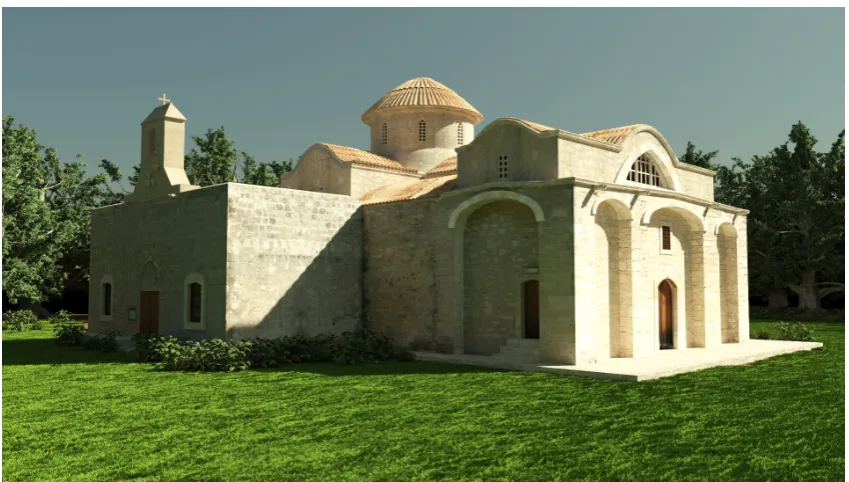
1.1 Rendering of a virtual scene using the efficient sky model proposed in Chapter 4. 2

2.1 Radiance . . . 6

2.2 Diffuse and specular reflection . . . 8

2.3 Path tracing . . . 13

2.4 Henyey-Greenstein Phase Function . . . 16

2.5 Importance Sampling Example . . . 18

2.6 Primary and secondary rays in Ray Tracing . . . 20

2.8 Light Tracing . . . 22

2.9 Bidirectional Path Tracing . . . 23

2.11 Path tracing . . . 27

2.12 Sketch of a neuron . . . 33

2.13 Sketch of an artificial neuron . . . 34

2.14 Non-linear classifier by using Kernels . . . 37

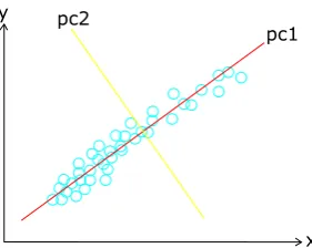
2.15 Principal Component Analysis on 2D . . . 38

3.1 Scattering of light coming from the left according to the Rayleigh phase func-tion for the particle posifunc-tioned at the origin. . . 41

3.2 Both of the figures illustrate the scattering of light coming from the left. Left: Henyey-Greenstein phase function. Right: Mie-Phase function. . . 45

3.3 The coordinate system used to define the sky models. . . 46

3.4 Environment map storing methods. . . 51

4.1 An illustration of 10 cloud types by Cloud Appreciation Society [25]. . . 65

4.2 A whole sky image captured with a fish eye lens. . . 65

4.3 Block division method by Cheng and Yu [21]. . . 71

5.2 Rendering of a car model with the proposed neural network sky model trained with the environment maps provided by Kider et al. [78]. . . 76

5.3 Coordinate system used for sun and view directions. . . 79

5.4 Mapping inputs to the RGB colour space with neural network. . . 81

5.6 Examples of the training of ANN with Preetham sky model . . . 85

5.7 Examples of the training of ANN with Hošek sky model . . . 86

5.8 Juxtaposition of the models in one image for different sun positions . . . 87

5.9 Skies for consecutive sun positions in a day in Egypt. . . 88

6.1 An illustration of the cloud modelling method. . . 91

7.1 Feature Extraction . . . 95

7.2 An illustration of clustering of feature vectors and labelling of the Representa-tive Feature Vectors. . . 99

7.3 An illustration of labelling the pixels. . . 101

7.4 Filtering of the misclassified pixels . . . 102

7.5 Accuracy of the method depending on the patch size and cluster size. . . 103

7.6 Concentric sampling from the labelled input. . . 104

7.7 Classification result of a cumulus cloud image. . . 105

7.8 Classification result of a stratocumulus cloud image. . . 105

7.9 Classification result of a cirrus cloud image. . . 106

7.10 Results for the mixed cloud image. . . 106

8.1 Overview of the method. . . 111

8.2 Illustration of the incident light from clouds. . . 112

8.3 Curved surface of the Earth and visible cloud bottom height level. . . 117

8.4 The cloud modelling algorithm . . . 119

8.5 A sketch of the cloud modelling algorithm. . . 120

8.6 Sketch of projection of clixels. . . 121

8.7 Clear sky behind the clouds. . . 121

8.8 Cloud modelling for cumulus cloud images. . . 127

8.9 Cloud modelling for cumulus cloud images. . . 128

8.10 Cloud modelling for stratocumulus cloud images. . . 129

8.11 Cloud modelling for stratocumulus cloud images. . . 130

8.12 Cloud modelling for cirrus cloud images. . . 131

Publications

Papers

Acknowledgments

I would like to express my gratitude to my supervisors Prof. Alan Chalmers and Dr. Kurt Debattista. I am grateful that they have given me the opportunity of having a PhD in the Visualisation Group. I would like to thank Alan for his constantly support, guidance, and trust. I also thank to Kurt for his patience, motivation and guidance during my PhD.

I am grateful to Thomas Bashford Rogers who gave me the courage to work on sky models. I also thank him for his patience, understanding and support during my PhD.

I also would like to express my gratitude to Prof. Emin Özça˘g and Prof. Ha¸smet Gürçay. Thanks a lot for trusting in me and also for prompting me to do the PhD in the University of Warwick.

I would like to thank to the Council of Higher Education (YÖK) and The Scientific and Tech-nological Research Council (TÜB˙ITAK), Turkey, for their financial support.

I would like to thank to Rossella who was always with me during this PhD. Thank you for endless support, deep conversations and cooking lessons. I would like to thank Ayten who supported me a lot with her wise advices and warm friendship. Thanks also go to Hilal and Musa who had been a family to me in England. I also thank to Debmalya and Emre for their sincere friendship. I also thank to Carlo for his support during my PhD and Jass for the amazing church model. I would like to thank to everyone in Visualisation Group for creating a scientific and a friendly environment: Amar, Jon, Josh, Tim, Ratnajit, Stratos, Emmanuel, Martin.

Abstract

Light sources are an important part of physically-based rendering when accurate imagery is required. High-fidelity models of sky illumination are essential when virtual environments are illuminated via the sky as is commonplace in most outdoor scenarios. The complex na-ture of sky lighting makes it difficult to accurately model real life skies. The current solutions to sky illumination can be analytically based and are computationally expensive for complex models, or based on captured data. Such captured data is impractical to capture and diffi-cult to use due to temporally inconsistencies in the captured content. This thesis enhances the state-of-the-art in sky lighting by addressing these problems via novel sky illumination methods that are accurate, practical and flexible. This thesis presents two novel sky illumi-nation methods where; the first of which focuses on clear sky lighting and the second one deals with illumination from cloudy skies.

The first approach compactly and efficiently represents sky illumination from both existing analytic sky models and from captured environment maps. For analytic models, the ap-proach leads to a low, constant runtime cost for evaluating lighting. When applied to envi-ronment maps, this approach approximates the captured lighting at a significantly reduced memory cost, and enables smooth transitions of sky lighting to be created from a small set of environment maps captured at discrete times of day. This makes capture and rendering of real world sky illumination a practical proposition. Results demonstrate less than 4% loss of accuracy compared to ground truth data. The straightforward implementation makes it possible to compute skies at sub milliseconds times on modest GPUs.

Chapter 1

Introduction

Demand for the creation of high-fidelity rendering of virtual scenes has grown rapidly in a wide range of domains such as architecture, computer games, civil engineering, enter-tainment, cultural heritage and advertising. In architecture, buildings could be predictively visualised and their impact assessed entirely virtually. High fidelity graphics enable rapid prototyping and evaluation of new design spaces. In computer games, there is a perpet-ual demand for increased realism and improved interactivity. For cultural heritage accurate graphics offer a glimpse into the past and help form a better understanding of such sites. In advertising, image synthesis is preferred when it is costly or difficult to generate a real-world scene. The accurate modelling of the light transport, materials and, in particular, light sources are a fundamental requirement for realistic graphics. This work focuses on the re-production of lighting, in particular the contribution of sky lights. In real life and in many application areas the sky is the main source of light and is, typically, solely responsible for outdoor and exterior lighting, and ,commonly, also interior lighting. Figure 1.1 shows an ex-ample of a scene entirely lit from the sky using a method developed in this thesis. The sky not only contributes to the lighting, it is not uncommon for the sky to occupy a large portion of the final rendered image. Accurate sky lighting contributes significantly to image synthe-sis and aspects of it have frequently been ignored in the literature. This thesynthe-sis focuses on modelling clear and cloudy sky illumination to facilitate different sky sources that are novel, efficient and customisable.

1.1 Motivation

such as dust, smoke and water vapour, and molecules such as oxygen, carbon dioxide and nitrogen each of which has a different impact on the light propagation. Light transport in an atmosphere requires an understanding of the physical processes underpinning light travers-ing the atmosphere. Sky lighttravers-ing is the result of the interaction of sunlight with particles in the air. Light can interact with particles in two ways: scattering and absorption. These in-teractions can change according to the optical properties of the particles. On a clear day, molecular absorption and scattering is observed. Water vapour, dust, smoke and other par-ticulate matter in the air are also responsible for the scattering of light in the atmosphere. Clouds contain a large concentration of water droplets and have a large impact on atmo-spheric light transport. Therefore, to be able to render virtual scenes accurately it is neces-sary to accurately render both clear skies and clouds.

In the field of computer graphics several methods have been introduced to generate arti-ficial skies. Commonly used analytic sky models have been proposed by Perez et al. [112], Preetham et al. [117] and Hosek and Wilkie [61]. These methods handle sky illumination with different haziness, sun position and scattering types. These models were derived by fitting coefficients to initial simulations of light scattering in the atmosphere. However, in computer simulations, computational efficiency and the collection and storage of data are very important limitations to be considered. Use of complex analytical models can be costly to compute interactively; an alternative to this is to capture sky environment maps which constitutes a laborious and impractical task, especially when considering smooth anima-tions are required.

can be obtained by using physically based participating media rendering techniques, Jensen and Christensen [72], Lafortune and Willems [90]. However, it is difficult to obtain an accu-rate 3D model of clouds which maintains their spatial and optical properties. The number of droplets in a specific volume (water content), the radius of the droplets and the depth of the cloud all affect the number of scattering events inside the cloud. Most research that has focussed on modelling and rendering of clouds has not accounted for the optical proper-ties of clouds. Additionally, most current approaches attempt to synthesise cloud volumes in an ad-hoc manner. Ideally, virtual clouds should be generated which reliably replicate real-world clouds.

1.2 Approach

This section provides an outline for the novel approaches to sky light modelling presented in this thesis. The first approach is an efficient representation of sky light models that also en-ables practical use of captured environment maps. The second approach focusses on cloud modelling. This approach includes two contributions to the literature. The first is a clas-sification of clouds from a single image at a per-pixel level, and the second, automatically generates 3D models of clouds via a single captured image; these clouds can then be re-lit virtually by any sky to produce synthetic environment maps that can act as light sources. The first approach in this thesis presents an alternative model for sky illumination based upon machine learning techniques. This method encodes the non-linear mapping of the sun and view direction to radiance values using a single layer Artificial Neural Network. The network is trained using a sparse set of samples which capture the properties of the light-ing at various sun positions. This allows for an efficient, both computationally, and in terms of memory, representation of analytic and captured skies, and results enable smooth ani-mations of lighting from a sparse set of captured environment maps. Results demonstrate accuracy close to the ground truth for both analytical and captured based methods. This ap-proach has a very low runtime overhead meaning that it can be used as a generic apap-proach for both off-line and real-time applications.

classi-fied skies provide initial information about the distribution of lighting in the scene. In the second step, an iterative optimisation technique is used to fit a 3D volume to the cloud pixels to match the colour of the input image. This allows virtual clouds to be synthesised which correspond to real world clouds, and can then be applied to arbitrary lighting environments. The results show that illumination by skies can be replaced by the fitted models and can be integrated with different atmospheric conditions to simulate lighting providing a broader range of lighting conditions to potential users.

1.3 Thesis Outline

(Chapter 2) Background provides the concepts relevant to this thesis such as light, light transport, physically-based rendering and machine learning.

(Chapter 3) Sky Light Modellingpresents an overview of light scattering and skylight mod-elling. This chapter also investigates the optical and geometrical properties of clouds, cloud classification and modelling techniques.

(Chapter 4) Discussion & Methodologyprovides a discussion on the techniques described in Chapter 3. Based on this discussion the methodology used in this thesis is presented.

(Chapter 5) A Machine Learning Driven Sky Modelpresents a novel method for skylight modelling based upon machine learning techniques which can learn, and reproduce, illu-mination from both the analytic sky models and environment maps.

(Chapter 6) Physically-Based Cloud Modellingprovides the motivation for the methods in-troduced in the following two chapters and outlines the broader method used for obtaining cloud models from a single captured image.

(Chapter 7) Classification of Cloudsproposes a novel method for per pixel classification of clouds from single HDR image captures.

(Chapter 8) Modelling of Clouds from a single HDR Imageintroduces a novel cloud mod-elling and illumination technique from an input HDR image. This method can be used in real time and with different sky scenarios.

Chapter 2

Background

2.1 Light

Computer graphics is concerned with the synthesis of imagery which is both visually plau-sible and physically accurate. This is achieved by the simulation of how light propagates around the scene and takes into account all interactions with the scene. Image synthesis requires certain inputs to be specified, namely: light sources, scene geometry (as well as de-scriptions of how this geometry reflects light) and a virtual camera which is used to view the scene.

2.1.1 Radiometry

The science dealing with the measurement of light is called radiometry. The main radiomet-ric quantities which are typically required in computer graphics are given below, following Dutre et al. [39] and Pharr and Humphreys [114].

• Radiant power(Φ) also known as flux is the quantity expressing how much light arrives at or leaves a point. It is measured inw at t s (W) (joules/sec).

• Irradiance(E) describes the measurement of the incident light per unit surface area. It is measured inW/m2.

E=dΦ

d A (2.1)

• Radiosity(B) is the exitant light per unit surface area. It is also expressed inW/m2.

B=dΦ

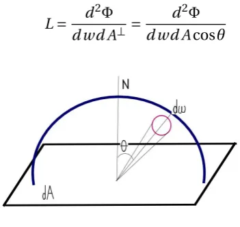
• Radiance(L) is radiant power per steradian per projected area,W/sr.m2.

L= d

2_Φ

d wd A⊥=

d2Φ

d wd Acosθ (2.3)

Figure 2.1: Radiance

In Equation (2.3)d A⊥expresses the projected area and the term steradian (sr) is the expres-sion of the solid angle, (Ω). Solid angle is the area of an object projected onto the unit sphere centered at a point x.

dω=d Acosθ

r2 (2.4)

Radiance is one of the most commonly used terms in computer graphics. According to the definitions of radiometric terms it is possible to represent each term by means of radiance. LettingL(x →Θ) be the radiance leaving the pointx, andL(x←Θ) to show the radiance arriving the pointxthrough the angleΘ, we can obtain the following equations.

Φ= Z

A Z

ΩL(x→Θ)cos(θ)dωΘd Ax (2.5)

E(x)= Z

ΩL(x←Θ)cos(θ)dωΘ (2.6)

B(x)= Z

ΩL(x→Θ)cos(θ)dωΘ (2.7)

An important property of radiance is that the incident and exitant radiance value between two points does not change. It means radiance remains same along a straight line if there is no particle in the air that will interact with the light.

2.1.2 Surface Interaction

In a realistic scene light interacts with the objects within the scene. This interaction can cause light to be scattered or absorbed (turned into heat energy) by the surface. These in-teractions depend on the material of the surface and wavelength of the light. To give an ex-ample, a material can absorb red and green wavelengths of light and scatter only blue light which will cause the blue appearance of the object. The brightness of blue depends on the scattering angle and view direction. The amount of the light scattered in a direction changes according to the material of the surface and explained by the Bi-directional Reflectance Dis-tribution Function (BRDF) and also by the Bi-directional Scattering DisDis-tribution Function (BSDF) which includes the transmittance of the light.

2.1.2.1 BRDF and BSDF

The way a surface reflects light ray depends on the surface material. In reality not all the light is reflected by the objects. Some of it transmits through the object or is absorbed (turns into heat energy). The rest is reflected because of the conservation of energy. The func-tion modelling the relafunc-tion between the incoming and reflected light is called the Bidirec-tional Reflectance Distribution Function (BRDF) (Dutre et al. [39], Cohen and Wallace [26]). In mathematical terms letwo be the exitant direction andwi be the incoming direction of

the light then the ratio between the differential radiance and differential irradiance is called BRDF shown asfr(x,wi→wo) :

fr(x,wi→wo)=

d L(x→wo) d E(x←wi)

= d L(x→wo)

L(x←wi)cos(Nx,wi)dωwi

(2.9) whereNis the surface normal.

The bidirectional scattering function (BSDF) is the generalization of BRDF and includes transmittance of light.

The BRDF satisfies the following important properties which are useful for rendering pur-poses:

1 Helmholtz Reciprocityimplies that the value of the BRDF will remain the same if the in-coming and outgoing directions of light are swapped.

fr(x,wi→wo)=fr(x,wo→wi) (2.10)

can be used by interchangingwiandwo:

fr(x,wi↔wo) (2.11) 2 Energy Conservationtells that the total outgoing reflected power must be less than or equal

to the incoming power on the surface:

Z

Ωfr(x,wi↔wo)cos(Nx,wi)dωwi ≤1 ,∀wi (2.12) 2.1.2.2 Surfaces

Figure 2.2: Reflection of light from specular (left), diffuse (middle) and glossy (right) surface Some common BRDF models are as follows, Figure 2.2:

Diffuse

Diffuse surfaces reflects the light uniformly over the hemisphere surrounding the hit point:

fr(x,wi ↔wo)=κ_πa whereκais the fraction of light reflected by the surface. Specular

If the material of the surface is specular then the light will be either reflected or refracted by the surface. For a surface with the normalN and light coming in the direction ofωi, the

direction of reflected lightRis given by the following equation:

R(N,ωi)=2(N·ωi)N−ωi (2.13)

Refracted light is found by Snell’s Law. At a transmissive surfaceηi andηt respectively show

the refractive indices of the external and entered medium. Also if we assume thatωi andωt

indicates the angle between the incident and transmitted light ray and normal of the surface, respectively, the relation between these quantities are given by the following equation.

Glossy surfaces describe the type of reflections typically exhibited by real-world objects. These BRDFs describe the situation where more light is reflected around a certain, typically the perfect reflection, direction. Some of these models are described below:

• Modified Phong: This model by Lewis [95] is an improved version of the Phong BDRF Phong [115]. This model combines the idea of diffuse and specular lobes - a term which defines the shape of Phong-like BRDF:

fr(x,wi→wo)=

κd

π +κs

e+2

2π (wo·R(N·wi))

e

(2.15) wheree is the specular exponent andN is the surface normal.

• Ward: This model by Ward [141] describes the reflection of light as a combination of specular and diffuse reflection from the surface and uses a term half angle to describe the angle betweenwi andwo:

fr(x,wi→wo)=

κd

π +κs

e

−t an2(θh) α2

4πα2p_(N·w

i)(N·wo)

(2.16) whereθhis the angle between surface normal and half angle,αdecribes the roughness

of surface andκd andκsare weights of surface diffuse and specular reflection.

• LaFortune: Lafortune et al. [91] used a mixture of Phong lobes to describe surface reflectance:

fr(x,wi →wo)=κd

π +κs

Nl obes

X

i=1

(wo·R(Wi,wi))ei (2.17)

whereWi is the orientation axis andei is the specular exponent of the i’th lobe and Nl obesis the number of lobes .

• Microfacet: In these BRDFs the surface is described as being composed of tiny mir-rored planar surfaces which are distributed probabilistically. Some common models in this class are the Torrance and Sparrow [133] model, the Cook and Torrance [27] model, and the Ashikhmin-Shirley model by Ashikmin et al. [5]. The Torrance-Sparrow model simulates the reflection of light from isotropic surfaces and defined as:

fr(x,wi→wo)=

κd

π + κs

4π(N.wi)

D(h)F(wo)G(Wo,wi) (2.18)

express the ratio of light reflected from the surface. The Cook-Torrance model is a more generalized version of the Torrance-Sparrow model with improved Fresnel and distribution functions. It can be applied to many material types with different sur-face conditions. The drawback of the method is to find the optimal input parameters to generate the desired output. The anisotropic BRDF model by Ashikhmin-Shirley model is mostly generalized reflectance model with a simple derivation.

• Empirical: These BRDF models typically consist of measured data of surface re-flectance encoded in a lookup table. Despite a general high accuracy of reproduction of real surfaces, these models frequently suffer from measurement errors, and a large memory consumption. To improve the efficiency of using of look-up tables, several methods have been introduced to compress the data or fit a model to the data such as LaFortune or Ward BRDF models.

2.1.3 Light Sources

A light source is an object in the scene which emits light. The type, colour and intensity of the light source can change the way we perceive the scene. Light sources emit radiance into the scene and are an essential part of rendering algorithms. Lights are described according to the directional distributionpe(x,w) of emitted light where

R

ωpe(x,w)d w=1. There are

several types of light sources commonly used in computer graphics, Pharr and Humphreys [114]:

• Point Lights: This light source is a single point within the scene and typically emits the same amount of light in every direction. This light source is given as a Dirac function in position, but emits in all directions. The emission is typically uniform over all direc-tions, but can be combined with an emission profile to model certain light sources in more detail.

• Directional Lights: This light source illuminates the scene from a single direction; that is it is a Dirac function in direction but without a defined position. A common use for this light source is to approximate lighting from the sun in a virtual environment. • Spotlights: Spotlights emit light in all directions which compose a cone. Similary to

Point Light sources, this light source can be textured or follow an emission profile. • Area Lights: These light sources have a specific geometry which emits light. Since the

visibility of a point by the light source will change according to the sampled point on the light source, rendering with area light sources gives more realistic scenes with soft shadows.

source is composed of an infinite number of directional lights which cover the full sphere of directions. These directions typically have a texture associated with them, and are commonly used to represent natural illumination or skies in rendering, and lead to plausible results when used to relight synthetic scenes. This method will be covered in more detail in Section 3.5.

2.2 Light Transport

Image synthesis requires the use of both direct and global illumination methods. In direct illumination a light path between the camera and light source includes only one interaction with the scene objects. Global illumination is more complicated where it simulates various paths of light interaction with the surfaces in a scene. An example of this is light bouncing off a red carpet onto a white wall, resulting in a red hue on the wall. In this section the mathematical models explaining the interaction of light with the objects in the scene and some common solutions to these models will be introduced.

2.2.1 The Rendering Equation

The rendering equation which is a formalism of the global illumination problem was intro-duced to computer graphics by Kajiya [74]. It formulates the outgoing radiance at a point by considering the incoming radiance and the surface reflection properties at that point. Radiance leaving a surface pointxin the direction ofwois the sum of emitted radiance and

reflected radiance at the point:

L(x→wo)=Le(x→wo)+Lr(x→wo) (2.19)

Light is reflected according to the following equation:

Lr(x→wo)= Z

Ωfr(x,wi→wo)L(x←wi)cos(wi)dω (2.20)

whered wis the differential solid angle.

Lastly by using Equation 2.20 with Equation 2.19, the rendering equation is obtained, Kajiya [74]:

L(x→wo)=Le(x→wo)+ Z

2.2.1.1 The Area Formulation

Equation 2.20 can be calculated over the surfaces of objects in the scene by using the Equa-tion 2.4 which is known as the area formulaEqua-tion:

Lr(x,x00)= Z

A

fr(x0→x→x00)L(x0→x)G(x0↔x)d Ax0 (2.22)

whereA is the set of all surfaces in the scene,x are points on the surfaces of the scene and

fr(x0→x→x00) is the BRDF of the surface written in three-point notation Veach [134].G(x↔ x0) is the geometry term to account for the change of variables from integrating over solid angle to integrating over area:

G(x↔x0)=V(x↔x

0_{) cos(N}

x,wi) cos(Nx0,−w_i)

∥x−x0_∥2 (2.23)

V(x↔x0) is a visibility term which accounts for visibility between two points in the scene. This is implemented by a ray casting operation:

V(x↔x0)=  



1 , if both of the points x and x’ are visible to each other 0 , otherwise

(2.24)

2.2.1.2 The Measurement Equation

The rendering equation formulates the transport of the light in a scene. However, the goal of rendering is to produce an image. Therefore, a final component of rendering an image is known as the measurement equation. This describes how the incoming radiance is weighted on the image via a functionWe:

Mj= Z

A Z

ΩWe(x,wi)L(x,wi) cos(Nx,wi)dωd Ax (2.25)

whereAis the area of the film.

2.2.1.3 The Path Integral Formulation

wherexi denotes a point on a surface (or can be generalised to a medium). The Path Integral

formulation integrates light transport over all paths of all lengths:

Mj= Z

P f( ¯x)dµ( ¯x) (2.26)

whereP is the union of all paths of all lengths and f is the product of emitted radiance, interactions with the scene, and connection to the camera, anddµ( ¯x) is a product of area measures. This integrand is expanded as follows (here for a path of lengthk):

f( ¯x)=Le(x0→x1)G(x0↔x1)

"_j=k−1 Y

j=1

fr(xj−1→xj→xj+1)G(xj↔xj+1)

#

We(xj−1→xj)

(2.27)

2.2.2 The Radiative Transfer Equation

Figure 2.3: Interaction of light with the medium.

So far, light has been described as if it travelling through a vacuum. However, in reality light typically travels through a medium, for example air or smoke. This medium is known as participating media. The Radiative Transfer Equation (RTE) by Chandrasekhar [20] describes the interaction of light with participating media. It describes the following interactions of light with a statistical distribution of the particles inside the medium:

• Absorption: When a light is absorbed by a particle it is converted to another form of energy such as heat. The probability of the light to be absorbed per unit distance is defined by the absorption coefficientσabs(m−1).

out-scattering. The probability of light to scatter at a unit distance is defined by the scat-tering coefficient:σsc a (m−1).

• Emission: Travelling of light in an light emitted media increases the radiance. Fire is an example of this kind of media where the heat energy is converted to light energy. This term is represented byLein this thesis.

Absorption and out-scattering of light causes the radiance L(x,w) received in a direction to reduce. This change is called extinction and is described by the extinction coefficient

σext =σabs+σsc a. The decrease in radiance due to extinction between two pointsxandx0

is described by the transmittance function:

Tr(x,x0)=exp−τ(x0,x) (2.28) whereτis the optical thickness of the medium. It is equal to the integral of the extinction coefficient over the line betweenxandx0: τ(x0,x)=R0dσext(x+t w)d t, whered =∥x−x0∥

andw is the normalized direction fromx to x0. For a homogeneous medium this takes a simple form:

Tr(x,x0)=exp−∥x−x0∥σext _(2.29)

The amount of light received in a direction is increased by in-scattered light. Therefore, by integrating over the sphere of all directions the in-scattered light in a directionwo can be

found:

Li(x→wo)= Z

ω℘(x,wi→wo)L(x←wi)d wi (2.30)

where℘is the phase function which describes the normalized angular distribution of scat-tering at a pointxin a medium (see Section 2.2.2.1).

Hence, the radiance at a pointxreceived from a directionwcan be written as:

L(x←w)=Lr ed(x←w)+Lem(x←w)+Li n(x←w) (2.31)

whereLr edis the reduced radiance coming from the background,Lemis the reduced emitted

Lr ed(x←w)=Tr(x0,x)L(x0→ −w) (2.32)

Lem(x←w)= Z x

x0

Tr(x0,x)σabs(x0)L0e(x0→ −w)d x0 (2.33) Li n(x←w)=

Z x

x0

Tr(x0,x)σsc a(x0)Li(x0→ −w)d x0 (2.34)

wherex0is a point outside the media (see Figure 2.3).

2.2.2.1 Phase Function

Angular scattering of particles in a participating medium is described by the phase func-tion. This gives rise to many optical properties of the medium. The simple case of medium where light scatters the equally in all directions is described by isotropic scattering. How-ever, most common media have anisotropic scattering properties. Scattering of light mostly in the forward and backward direction is called forward-scattering and backward-scattering, respectively. These are typically represented by the Henyey-Greenstein and Schlick phase functions.

Isotropic Phase Function

The isotropic phase function describes scattering of light equally in all directions. Since the phase function is normalized, its integral over the sphere of directions is 1:

Z

ω℘I(x,w,w

0_{)d w}0_{=1 (2.35)}

which makes℘I take a constant value of 1/4πfor all directions. Henyey-Greenstein Phase Function

g=0. g=0.45 g=-0.45

0

:

:/2

2:/3

Figure 2.4: Scattering of light coming from left according to Henyey-Greenstein Phase Function for the particle positioned at the origin.

The function is defined as:

℘hg=

1−g2

4π(1+g2_{−2gcos(θ))}1.5 (2.36)

Schlick Phase Function

A computationally efficient version of the Henyey-Greenstein phase function was derived by Blasi et al. [11]. This simplified version calculates the forward or backward scattering with a parameterk∈[−1, 1]:

℘s=

1−k2

4π(1+kcosθ)2 (2.37)

where the negative values ofkgive backward and positive values give forward scattering.

2.3 Monte Carlo Methods

Integrals such as the Rendering Equation, Equation 2.21, cannot be evaluated analytically except for simple and unrealistic scenarios. Therefore, numerical integration methods, es-pecially Monte Carlo, are used to solve this type of integral. As Monte Carlo integration is based on probability theory some concepts on probability theory by DeGroot and Schervish [31] and Veach [134] are presented.

Cumulative distribution function (CDF) P(x)of a random variable x is defined as

P(x)=P r(X ≤x)= Z x

−∞

p(y)d y. (2.38)

Expected Value (E[x])andVariance (V[x])of a random variable x are defined as

E[x]= Z ∞

−∞

xp(x)d x. (2.39)

V[x]=E[(x−E[x])2]= Z

(x−E[x])2p(x)d x. (2.40) These concepts are used in Monte Carlo integration. Consider the following integral:

I= Z b

a

f(x)d x. (2.41) This can be numerically evaluated using Monte Carlo by choosing random points from a PDFp:

ˆ

I= 1

n n X

i=1

f(xi) p(xi)

. (2.42)

where n is the number of samples (xi) taken from the domain of the integralI with

proba-bilityp(xi). The expected value of the function ˆIis shown to match the actual value as, E[ ˆI]=E

·

1

n n X

i=1

f(xi) p(xi) ¸

= 1

n n X

i=1

E

·

f(xi) p(xi) ¸

= 1

nn

Z

.f(x)

p(x)p(x)d x=

Z

f(x)d x=I (2.43) Since the expected value of the function ˆI is equal to the integralI, we can use ˆIto evaluate the value of the integralI.

2.3.1 Stratified Sampling

Stratified sampling partitions the domain of the integral into subdomains, and places sam-ples in each sub domain. The estimator is then the sum of the estimates of f in each subdo-main:

Z D

0

f(x)d x= Z D₁

0

f(x)d x+ Z D₂

D1

f(x)d x+...+ Z Dn

Dn−1

f(x)d x (2.44) It can be shown that that variance of stratified sampling is always less than or equal to stan-dard Monte Carlo. This is commonly used in graphics to distribute samples over the image plane, where each subdomain corresponds to a pixel.

2.3.2 Importance Sampling

Figure 2.5: Applying importance sampling to reduce the noise in the image. The same scene without (left) and with (right) importance sampling based on the intensity of the textured

light source.

Importance sampling is a powerful variance reduction technique which uses a PDF which is as close to proportional to f as possible. Consider two situations, one with a constant

p(x) over the domain of integration and another which roughly matches the shape off. If f

intensity of the textured area light source versus uniformly sampling the domain. The image on the right shows the variance reduction properties of importance sampling.

2.3.3 Multiple Importance Sampling

Multiple importance sampling by Veach and Guibas [136] is a variance reduction method commonly applied to computer graphics. In some cases the integral in Equation 2.41 in-cludes the product of several functions such as:I=R f(x)g(x)d x. In this case it is not always possible to find a common distribution to sample points. Multiple Importance Sampling proposes to sample from separate distributions and use the following estimator:

m X

j=1

1

nj nj

X

i=1

f(xi j)Wj(xi j) pj(xi j)

(2.45) wherenj is the number of samples drawn from the distributionpj andmis the number of

distributions in the estimator.W is the weight to control the variance in case the distribution

pis a poor representative of f. Note,Pm

i=1Wi=1. A generally optimal choice for the weight

is balance heuristic:

Wj(x)=

njpj(x) P

inipi(x)

(2.46)

2.3.4 Other Methods

Importance Sampling and Multiple Importance Sampling are the most commonly used method in computer graphics. Other approaches have found some use for variance reduc-tion:

• Control Variates: These subtract a functiong which approximately matches the shape of f and integrate the difference: E[f(x)]=RD f(x)−g(x)d x+

R

Dg(x)d x. Therefore,

the variance is proportional to the difference off andg, and ifg matches f well, this variances can be much lower than that of integrating over f.

• Sampling Importance Resampling: This generates a large number (N) of samples drawn from one distribution, which are then weighted by another distribution. M

2.4 Physically Based Rendering

Synthesis of imagery based on the principles outlined in this chapter is known as rendering. The following sections outline common rendering approaches for surfaces and participating media, with a focus on those used in this thesis.

2.4.1 Rasterization

The main idea behind rasterisation is to project the geometry of the scene, typically triangles, onto the image plane. To resolve visibility for the primitive, the depth of each fragment is compared to the previously stored depth (if it is less, then it is visible) using a data structure called a z-buffer. The colour values stored at the vertices of the primitives are interpolated in order to shade the fragment. This technique is useful when one needs speed but on the other hand it cannot naturally deal with all types of light transport such as reflection, refraction and global illumination. Therefore, it is not considered further in this thesis.

2.4.2 Ray tracing

Figure 2.6: Primary and secondary rays in Ray Tracing

shown in the Figure 2.6. This method produces more realistic lighting effects compared to Appel [3] such as shadows and refractions.

2.4.3 Path Tracing

Figure 2.7: Path Tracing

Path tracing was introduced by Kajiya [74]. This is based on using the ray tracing methodol-ogy with additional stochastic sampling in order to simulate full global illumination effects. The central idea is to calculate the contribution of all possible light sources to the current hit point and let the ray to bounce until a stopping criteria is met.

L(x→wo)=Le(x→wo)+Ld(x→wo)+Li d(x→wo) (2.47)

whereLe is the light emitted directly from the point,Ld is direct lighting andLi d is indirect

lighting, see Figure 2.7. The direct illumination corresponds to evaluating the radiance di-rectly coming from the light source. This is known as Next Event Estimation. For each hit point in the scene, a point on the light source is sampled and the visibility between the hit point and the point sampled on the light source is computed. Direct lighting is calculated as:

Ld(x→wo)=

1

N N X

i=1

fr(x,wi→wo)Le(x←wi)cos(Nx,wi) pd(wi)

(2.48) whereLei is the incident radiance in the direction ofwi, andpd(wi) is the PDF of sampling

the light source in the directionwi.

using the reflected lightLr, see Equation 2.20: Li d(x→wo)=

Z

Ωfr(x,wi →wo)Lr(x←wi)cos(Nx,wi)d wi (2.49)

This tracing process needs a stopping condition to prevent paths from having an infinite length. For this purpose Russian Roulette is used as an unbiased stopping condition. Path tracing can compute all indirect light paths except those from point light sources seen though specular surfaces, as the probability of generating these paths is zero.

The rendering steps of path tracing is explained in Algorithm 1.

Algorithm 1Path Tracing Algorithm

1: foreach pixel in the image planedo

2: Compute the ray direction from eye through the pixel

3: Find the first intersection point of the ray with scene

4: Compute direct illumination valueLd

5: whilenot terminateddo

6: Sample a new directionw

7: Compute indirect illuminationLi din the direction ofw

8: Find the first intersection point of the ray with scene

9: Compute direct illumination valueLd

10: Decide to terminate path

2.4.4 Light Tracing

Figure 2.8: Light Tracing

2.4.5 Bidirectional Path Tracing

Figure 2.9: Bidirectional Path Tracing

This method by Veach and Guibas [135] and Lafortune and Willems [89] generalizes both path tracing Section 2.4.3 and light tracing Section 2.4.4. It combines the advantages of the paths that these two methods can generate. In this method two paths are generated simultaneously, one from the light source (light pathxLof lengthNL) and another is from the

eye (eye pathxE of lengthNE) and the end point of each subpath is combined. Ifi<NE and j<NL are indices of path vertices on the eye and light paths respectively, a path is created: xE(i)xL(j). Each connection between the two subpaths evaluates the geometry term and

BRDFs of the vertices at the end of each subpath. This path then has to be weighted by all the possible ways it could have been created. For example, the same path could have been generated usingi−1 light path vertices and j+1 eye path vertices. In order to reduce variance, Multiple Importance Sampling is used to weight the sampled combination against all the possible combinations of subpath vertices. This process is repeated for allNE andNL

vertices, and is illustrated in Figure 2.9.

2.4.6 Metropolis Light Transport

Metropolis Light Transport by Veach and Guibas [137] is another approach to solving global illumination problems. This method is similar to the idea in the Metropolis Sampling algo-rithm. Initially a set of pathsx0,x1, ...,xN are generated (the authors used bidirectional path

tracing for this purpose). These paths are mutated by deleting, adding or replacing subpaths according to the Metropolis Hastings algorithm.

are efficient at exploring regions of path space which make a high contribution to the image plane, such as caustics. InLens Subpath Mutationa subpath which ends at the eye is cho-sen to be deleted and replaced. This mutation type helps to stratify samples over the image plane.

The MLT algorithm works as follows:

Algorithm 2Metropolis Light Transport Algorithm, by Veach and Guibas [137]

1: Specify an initial pathX

2: setimageto an array of zeros

3: forj←1 toNdo

4: Y ←mut at e(X)

5: a←Accep t P r ob(Y |X)

6: Generate a random numberU

7: ifU<athen

8: setX ←Y

9: Recor d Sampl e(image,X)

10: Returnimage

There has been research into enhancing the MLT algorithm. Cline et al. [24] created short chains of mutations and improved stratification over the image plane. Kelemen et al. [76] used Primary Sample Space to mutate a path. Primary Sample Space consists of the unit hy-percube of random numbers, and a single coordinate in this space defines a path. Two types of mutation strategies are defined in this approach: small mutations make slight changes to the random numbers which generate a path, and large mutations generate a new set of random numbers and therefore a new path, which ensures ergodicity.

2.4.7 Photon Mapping

Figure 2.10: Photon Mapping.

at each hit point. To perform efficient lookups in the second step, the photons are stored in a kd-tree structure. In the second step, rays from the camera are shot into the scene and for each hit point the flux of the photons within an area of the hit point are used to evaluate the radiance coming to the camera. By using density estimation from the stored photons, the exitant radiance at a pointxis estimated:

L(x→wo)= n X

p=1

fr(x,ωo,ωi)∆φp(xo,ωi)

πr2 . (2.50)

whereris the radius of the sphere containing thennearest photons,∆φpis the flux received

by the pointxcoming from the photon p in the direction ofωi andωois the outgoing

di-rection. This method is limited by the number of photons that can be stored in the memory. It also generates biased results, but consistent. To reduce the low frequency noise, a final gathering is commonly implemented: rays are sent from the camera and at each primary hitpoint, the BRDF is sampled and rays are shot. Density estimation is used to calculate the outgoing radiance at each of the secondary hitpoints.

2.4.8 Progressive Photon Mapping

This method by Hachisuka et al. [51] solves the memory issues of Photon Mapping. As a first step, rays are shot from the eye to calculate primary hit points. These hit points store information describing the position, flux and radius. In subsequent passes, photons are shot from the light sources. When a photon falls within the footprint of a hit point from the first pass, its transported flux is added to the stored quantity at each hitpoint. Additionally, the radius is reduced such that the estimate converges in a consistent manner. This is expressed as:

L(x→wo)≈

1

4A n X

p=1

fr(x,ωo,ωi)4φp(xp,ωi)=

1

πR(x)2

τ(x,ωo) Nemi t t ed

(2.51) whereτ(x,ωo) is the sum of multiplication of the BRDF and unnormalized flux forNphotons

at the pointx.

2.4.9 Irradiance Caching

estimated error exceeds a threshold. A cache entry is computed via Monte Carlo sampling of light paths over the hemisphere surrounding the cache point. As this method stores irradi-ance, Irradiance Caching can only be applied to diffuse surfaces.

Irradiance caching was extended glossy surfaces in the radiance caching algorithm Krivanek et al. [86]. This method is used to render scenes with low frequency glossy surfaces and uses spherical harmonics to represent the incoming radiance.

2.4.10 Instant Radiosity

Instant radiosity by Keller [77] shoots paths from the light source into the scene and at each hit point stores a point light source, known as a Virtual Point Light (VPL), on the surfaces. A second pass approximates both direct and indirect lighting as the average of the lighting contributions from each VPL:

L(x→ωo)=

1

Nv pl s Nv pl s

X

i=1

Li(xi→x)f r(x,wi →wo)G(xi↔x) (2.52)

whereN_{v pl s} is the total number of stored VPLs,Li(xi →x) is the emitted light from thei0t h

VPL in the direction tox. xi is the position of thei0t h VPL andwi is the direction from the

VPL to the hit pointx.

The accuracy of this method depends on the number of virtual light sources. As the number of light sources increases, the computational cost required to produce images also increases. To deal with this problem, many lights methods have been proposed which do not use all VPLs to reconstruct the image, but use a subset which minimise some error metric, such as Walter et al. [140].

2.4.11 Vertex Connection and Merging

2.5 Rendering of Participating Media

As the focus of this thesis is on participating media, in this section some of the common participating media rendering techniques will be presented.

2.5.1 Monte Carlo Approach to Volumetric Path Tracing

PARTICIPATINGMEDIUM

Figure 2.11: Path tracing in a medium.

Path tracing based approaches can be extended to render participating media. Equation 2.31 can be solved by Monte-Carlo techniques by rewriting it as follows:

L(x←w)= Z x

x0

Tr(x0,x)

·

σsc a(x0)Li(x0→ −w)+σabs(x0)Le(x0→ −w) ¸

d x0

+Tr(x0,x)L(x0→ −w)

(2.53) For a non-emissive medium the solution of this equation requires solving the following in-tegral:

L(x←w)= Z x

x0

Tr(x0,x)σsc a(x0)Li(x0→ −w)d x0 (2.54)

The Monte-Carlo solution of this integral requires to sample scattering points and directions for each scattering points:

L(x←w)≈ 1

N N X

j=1

Tr(x0_j,x)σsc a(x0_j)Li(x0_j → −w) pt r(x0_j)

(2.55) wherept r is the probability of sampling a pointx0along the ray starting fromxin the

The direction of in-scattered radiance is sampled proportionally to the phase function℘ph: Li(x0j→ −w)≈

1

M M X

n=1

℘(x0_j,wn→ −w)L(x0_j ←wn) pph(wn)

(2.56) whereMis the number of sampled directions.

The steps of rendering a non-emissive medium are given in Algorithm 3.

Algorithm 3Volumetric Path Tracing Algorithm

1: foreach pixel in the image planedo

2: Specify the ray directionwfrom eye (x) through the pixel

3: L←Lr ed .Attenuated light coming from the

background, see Equation 2.31

4: p t←σsc a(x0)/pt r(x0) .Sample a pointx0along the ray

in-side the medium with probability

pt r(x0)

5: whileinsidedo

6: p t←Tr(x,x0_{)∗p t}

7: Lv_d(x0←wi)=Tr(x00,x0)Le(x00→ −wi) .Attenuated direct light where the

light source (x00) is sampled from the phase functionpph(wi)

8: L←L+p t∗℘(x0_,w

i→w)∗Lv_d(x0←wi)/pph(wi)

9: p t←pt∗℘(x0,wnew→w)/pph(wnew) . Sample a new direction from the

phase functionpph(wnew)

10: w←wnew .Change the directionwtownew

11: Decide to terminate path

12: ifterminatedthen

13: break

14: x←x0 .Change the current point tox0. Up-date the ray.

15: x0←xnew .Sample a new point (xnew) along

the ray with probabilitypt r(xnew)

16: ifnot insidethen

17: break

18: p t←p t∗σsc a(x0)/pt r(x0)

2.5.1.1 Sampling of the Phase Function

The scattered direction at a point is sampled proportional to the phase function. Since the phase function is normalized and defines the probability of scattering in a directionw, the sampling probabilitypof directionw is the same as the value of phase function atw. Since the isotropic phase function has a constant probability of scattering, all of the directions will be sampled uniformly over the sphere with the same probability of 1/4π.

Samples can be drawn from Henyey-Greenstein phase functions by considering the anglesθ andφseparately, Pharr and Humphreys [114]. For two random variablesηandζifg6=0:

θ=cos−1

³−1 |2g|

³

1+g2−

³ 1−g2

1−g+2gζ

´2´´

(2.57) otherwiseθ=cos−1(1−2ζ) andφ=2πηwith the probability of samplingp(φ)=1/2π.

2.5.1.2 Distance Sampling

According to the properties of the media a scattering point can be sampled along the ray proportional to the transmittance between the current (x) and new point (x0). For a homo-geneous medium transmittance is simplified toTr=e−tσext _{wheretis the distance between}

two points. The probability of sampling a point in a homogeneous medium is:

p_ohom(x0)= Tr(x,x

0₎ R_∞

0 Tr(y)d y

= e

−tσext

R∞

0 e−tyσextd y

=σexte−tσext

(2.58)

Algorithm 4Distance sampling with Woodcock tracking

INPUT: A ray starting at x with direction of w and length d

DistanceSamplingWoodcockTracking(x,w,d)

1: t=0

2: whileη>σext(x+t∗w)/σl ar g e do

3: ξ=r and()

4: t=t−l og_{σl ar g e}(1−ξ) 5: ift>dthen

6: break

7: η=r and()

Algorithm 5Estimating the transmittance with Woodcock tracking

INPUT: A ray starting at x with direction of w and length d

TransmittanceEstimateWoodcockTracking(x,w,d)

1: t=Di st anceSampl i ng W ood cockTr acki ng(x,w,d)

2: returnt>d

A commonly used technique known as Woodcock tracking for distance sampling in hetero-geneous media was developed by Woodcock et al. [147] and introduced to computer graph-ics by Raab et al. [118], Algorithm 4. In this method random points (x) inside the volume are iteratively sampled until the following probabilistic condition is achieved for a random variableζ:

ζ>σext(x)/σl ar g e (2.59)

whereσl ar g e is the largest extinction coefficient of all the points inside the volume. In this

method more points are sampled at dense areas where the extinction coefficient is larger since the ratio is smaller at these areas. Transittance estimation using Woodcock Tracking is shown in Algorithm 5.

Algorithm 6Estimating the transmittance with Ratio tracking

INPUT: A ray starting at x with direction of w and length d

TransmittanceEstimateRatioTracking(x,w,d)

1: t=0

2: T=1

3: whilet r uedo

4: ξ=r and()

5: t=t−l og_{σl ar g e}(1−ξ) 6: ift>dthen

7: break

8: T =T∗(1−σext(x+t∗w) σl ar g e )

9: returnT

Transmittance estimation based on Woodcock tracking was improved by Novák et al. [108] who continuously perform sampling steps until the ray leaves the medium, Algorithm 6. The transmittance along the path is accumulated in an efficient and unbiased manner, and is useful for estimating transmittance in large heterogeneous volumes.

2.5.2 Volumetric Photon Mapping

are stored in separate kd-trees which improves the efficiency of lookups. The inscattered radiance is estimated in two parts: direct and indirect. The indirect part is calculated as follows:

Li,i(x,→−w)≈(1/σsc a(x)) n X

p=1

℘(x,→−w0_p,→−w)∆Φp,i(x,

− →_w0

p)

4 3πr3

(2.60) where the summation is implemented on the smallest volumeV =4₃π/r3containing then

nearest photons and∆Φp,i is the flux that carried by these photons.℘is the phase function

andσsc ais the scattering coefficient. .

The in-scattered radiance is calculated by summing the direct lightingLi,dand weightedLi,i: Li(x,−→w)≈Li,d(x,w)+σsc a

(x)

σext(x)

Li,i(x,−→w) (2.61)

whereσext is the extinction coefficient.

2.5.3 Radiance Caching for Participating Media

In this method Jarosz et al. [68] used cache entries stored inside the volume to calculate the inscattered light. Cache entries are stored in an octree and keeps the information about in-scattered radiance, gradient and valid radius. A cache point is used in extrapolation of the query locations if they are within the valid radius. Since the inscattered radiance is the light leaving the point, it is stored over a sphere of directions and represented with spherical har-monics. The following exponential extrapolation is used to calculate the outgoing radiance at a given point:

L(x)≈exp(

P k∈C

³

ln(Lk)+∆_LL_kk(x−xk) ´

w(dk) P

k∈C w(dk)

) (2.62) whereL,xandr represent the radiance, gradient, position and radius for each cache point