An Experimental Forecasting Model

An Experimental Forecasting Model

Steven C. Ang, and Prof. Joan C. Manahan,

Member, IAENG

Abstract: Forecasting is fundamental to any planning effort. In the short run, a forecast is needed to predict the requirements for materials, products, services, or other resources to respond to changes in demand. The goal of this research is to present several forecasting techniques and models that are commonly used in business and to apply these techniques and models to create a new forecasting model with minor error. From the results in this research among the four main equations generated, the third equation

(

c+bx+ax2

)

(

1−V

) ( )

+ VA has the

most satisfactory results, in terms of MAPD, MAD and RMSE. In contrast to exponential smoothing, the generated equation is more objective in nature because of the multiplier used. The multiplier should be solved using the formulas

t t

t

A

A

A

−

₋₁ or

A

_t

−

A

_t−1

A

_t−1(among the two the first formula shows higher accuracy/precision than the second formula, most of the time), unlike in exponential smoothing, where the smoothing constant is based on the forecaster’s decision/perception.

Keywords: accuracy, degree of error, experimental forecasting technique, objective

1. INTRODUCTION

Forecasting plays an important role in all aspects of business, especially in the manufacturing of goods; forecasting is the basis of planning, in the functional areas of finance and accounting. A forecast provides the basis for budgetary planning and cost control. Production and operations personnel use forecasts to make periodic decisions involving process selection, capacity planning, and facility layout, and to make continual decisions about production planning, scheduling, and inventory. Three of the most widely use forecasting methods are the moving average, regression analysis, and the exponential smoothing.

The need for this research was simple and this was to find a more optimal forecast by decreasing the error that was present in every result that the forecaster would obtain.

Steven C. Ang Cell phone: +639162872293; e-mail: [email protected]

Prof. Joan C. Manahan is with the Industrial Engineering and Engineering Management Department, Mapua Institute of Technology, Muralla St., Intramuros, Manila, Philippines, Cell Phone: +639206639399, e-mail: [email protected]

This might sound easy at first but actually formulating a model that would be more accurate than the existing forecasting method would take some time. Another need for this research was to truly understand the behavior of the demand and the factors affecting it. The authors observed the behavior of the demand is mostly unstable. This indicates that demand does not always come in a straight line or is not always linear. The only time that the data are in a straight line is when the uncontrollable factors are not considered, but in reality these uncontrollable factors are always present and affect the demand most of the time, and is one of the sources of error in every forecast. Therefore the objectives of this research focused not only in formulating a possible tool for forecasting, but also in understanding the behavior of the demand which was a part of the model to be formulated. The reason behind this was to actually relate the factors to the model and at the same time to show how it would affect the behavior of the model with regards to the demand and also in relation to the corresponding error associated with these factors.

2. METHODOLOGY

Using different forecasting techniques will helped the author to understand the behavior of the forecast patterns, its increase and decrease over a period of time. Selecting the best among different techniques would not be enough to obtain an optimal result desired. Using weights, the accuracy of a forecasting model, would be improved. The study concentrated on the selection of the forecasting technique with the highest forecast accuracy.

When forecasts are made, there is no way of knowing if they will be accurate enough to fit the actual values. By far, the most important attribute of a forecasting model is the accuracy of its forecasts. So with the use of three measures of error to understand and to know how accurate the forecasting technique would be. The first was the MAD which simply determines the average of the difference between the forecast and the actual demand. It indicates the nearness of the forecast to the actual values. This is best suited to systems in which the costs of forecast deviations depend on their cumulative effect regardless of whether the MAD is attributed to several small errors or a few large ones. The second was the MAPD which is used to measure the absolute error as a percentage. This shows the accuracy by means of magnitude and it shows proportion of the error to the actual values. The third was the RMSE, which is the square root of the sum of the squared forecast errors divided by the number of period N or simply the square of the MSE.

The experimenters used 20 sample companies, for gathering the data needed to produce a corresponding forecast and compare them with the actual data coming from the companies and the forecast that will be coming from the formulated models. By comparing the results from the 20 samples, it was determined that the difference in accuracy of each of the forecasting techniques or models used in the study. The author had resorted to a number of steps in formulating the model.

2.1 Determine what to forecast

The “what” to forecast comes in when the forecaster already knows why he/she must forecast. These are the “what material to buy” and the “what products to sell”. Basically this is what the forecaster needs to know for him to forecast.

2.2 Establish Time Dimensions

There were two types of time dimensions considered. The first was the number of periods the forecast should cover. For annual forecasts this might be from one to five years or more, although forecasts beyond

a few years are likely to be influenced by unforeseen events that are not incorporated into the model used. Quarterly forecasts are probably best used for one or two years (four to eight quarters), and monthly forecasts are suited to relatively short periods as well (perhaps as long as 12 to 18 months). This study used the quarterly forecast. The Second was the urgency of the forecast. Is it needed tomorrow? Is there ample time to explore alternative methods? Proper planning is appropriate here. If the forecaster can plan an appropriate schedule. This obviously will contribute to generating better forecasts.

2.3 Database Considerations

The data necessary in preparing a forecast may come from within or may be external. The first that was considered was internal data. Some people may believe that internal data are readily available and easy to incorporate into the forecasting process. But often this turns out to be far from correct. Data may be available in technical sense yet not readily available to the person who needs them to prepare the forecast. Or the data may be available but not expressed in the right unit of measurement (in sales pesos rather than units sold). Data are often aggregated across both variables and time, but it is best to have disaggregated data. For example, data may be kept for refrigerator sales in total but not by type of refrigerator, type of customer, or region. In addition, the data that are maintained may be kept in quarterly or monthly form for only a few years and annually thereafter. Such aggregation of data limits what can be forecast and may limit the appropriate pool of forecasting techniques.

2.4 Forecast Preparation

At this point, some method or set of methods have been selected for use in developing the forecast, and testing. It is recommended to use more than one forecasting method when possible, and it is desirable for these to be different types. The methods chosen should be used to prepare a range of forecasts. To prepare a worst-case forecast, a best-case forecast, and a most likely forecast.

2.5 Data Application and Testing

After preparing the techniques to be used, this is where the data gathered would be run in each of the techniques.

2.6 Model Selection

2.7 Model Formulation

The model was formulated using weights or multiplier to enhance the accuracy of the model. The weight is a representation of the error present in each of the periods that must be remove and be replaced by an equivalent amount of forecast that is needed, which may result to a more accurate or precise forecast.

2.8 Model Testing

After the formulation of the model, it was being tested using the same data applied in the forecasting model to maintain consistency of data and accurateness.

3. RESULTS AND DISCUSSION

The main idea of the model is to get the forecast values needed for the period; the remaining of the forecast was considered as error or unwanted forecast. Although this was the case, the weight (multiplier) computed was used to replenish an equivalent amount of forecast values which was taken from the actual values for the period or from the most recent forecast values.

So

Mi

was equal to

t t

t

A

A

A

−

₋₁ (1)

Where

A

_tis the actual value for the period and

A

_t−1was the actual value from the previous period.

A

_t

−

A

_t−1 . This equation represents the deviation from these periods. It was the difference between the two periods, which means it could be considered as the value equal to error, error which is always present in every equation, model or technique. Now by making it an absolute value, the value was also considered as the mean absolute deviation for that period, using this value as it is, would just make the model more complicated to understand. The values would only increase, so by dividing it by either

A

_t or

A

_t−1, the value would be in decimal form, which could be used to acquire the percentage value of the forecast needed and forecast to be added to replenish the unwanted forecast.

Let x be the selected forecasting technique to be improved or to be used for the experimental model. By letting

)

(

)

1

)(

(

x

−

Mi

+

MiA

(2)

be the equation for the experimental forecasting model, where

(

1

−

Mi

)

is the percentage or weight

of the forecast needed, since

Mi

is the percentage or weight of unwanted forecast or error so by subtracting it to 1, the amount needed will be equal to

(

1

−

Mi

)

, and thereby multiplying

(

1

−

Mi

)

to x, the amount equivalent to forecast needed would be acquired, but this value was still incomplete because it was not 100%, since it only got a percent equivalent to

)

1

(

−

Mi

, it still lacked a percent equal to

Mi

, therefore

(

MiA

)

would be added to compensate for the percent lacking in the equation. AHere is the value of the actual value for the period. Here

Mi

would not be representing error but an amount or percentage equal to the forecast value that needed to be replenished, since in the first half of the equation only

(

1

−

Mi

)

of the forecast was present, therefore the experimental forecasting model would be written as

(

x

)(

1

−

Mi

)

+

(

MiA

)

.

The author was able to come up with four combinations of the experimental forecasting model, to see whether there would be any change in the outcome. The first was the formulation of equation before

(

x

)(

1

−

Mi

)

+

(

MiA

)

; second, the author interchanged

(

1

−

Mi

)

and

Mi

, therefore having

(

x

)

Mi

+

(

1

−

Mi

)(

A

)

; the third was instead of

Mi

the author usedV , V is the average of all the

Mi

in the forecast. Since

Mi

was only for the individual forecast in each of the periods, the author noticed that there was no value for the following periods after the 8th periods and the result was either a zero or was the forecast value in x, which was why the author thought of using the average of the Miso that there would be corresponding values for the next periods after the 8th _{forecast values. The fourth and}

[image:3.612.308.518.483.670.2]

last equation was the same as the first but instead of

Mi

, V was used.

Table I: Actual Values for Alaska Milk Corporation

Forecast Values

Using the third equation

Forecast Values Using the third equation

Qtr Actual Values(in thousands of

pesos)

1 1 − − − =At At At

Mi Mi=A_t−A_t−1 A_t

1 1,170,081.00 1,186,884,345.80 1,187,149,291.94

2 1,234,614.00 1,253,484,591.84 1,253,782,133.20

3 1,230,323.00 1,306,698,388.93 1,307,902,635.07

4 1,774,651.26

8 1,457,237,403.46 1,452,232,592.05

5 1,256,591.00 1,416,237,268.82 1,418,754,485.48

6 1,481,560.00 1,507,421,351.91 1,507,829,119.82

7 1,419,894.00 1,546,164,031.51 1,548,154,989.58

8 1,762,820.00 1,656,406,885.71 1,654,729,020.85

9 1,388,029,688.82 1,409,915,395.79 10 1,434,691,940.48 1,457,313,392.79 11 _{1,480,308,342.13 1,503,649,049.36} 12 1,524,878,893.75 1,548,922,365.52 13 1,568,403,595.35 1,593,133,341.25

[image:4.612.93.305.527.706.2]

(

) ( )

(

)( )

(

)( )

(

)

(

)(

)

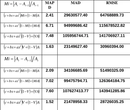
345.80 1,186,884, 000 , 081 , 170 , 1 2 0.17930662 2 0.17930662 1 2 0 637174.64 -0 45 . 67689076 17 . 1190555572 1 2 ax bx c .17 1190555572 c 5 67689076.4 b -637174.64 2 0.17930662 7 241515 . 0 041622 . 0 179031 . 0 291922 . 0 442427 . 0 003476 . 0 055153 . 0 0.241515 7 894 , 419 , 1 894 , 419 , 1 820 , 762 , 1 7 0.041622 6 0.179031 5 0.291922 4 0.442427 3 0.003476 2 0.055153 1 081 , 170 , 1 081 , 170 , 1 614 , 234 , 1 1 1 1 = + − ⎥ ⎥ ⎥ ⎥ ⎦ ⎤ ⎢ ⎢ ⎢ ⎢ ⎣ ⎡ + + + − ⎟ ⎠ ⎞ ⎜ ⎝ ⎛ _{+ +} = = = = ⎟ ⎟ ⎟ ⎠ ⎞ ⎜ ⎜ ⎜ ⎝ ⎛ + + + + + + = ∑ = = − = = = = = = = − = − − − = VA V a V V i M V M M M M M M M M M t A t A t A i M

Table II: Forecast Error generated by each of the models

1 1 − − − =At At At

Mi MAP

D

MAD RMSE

(c+bx+ax2)Mi+(1−Mi)A _{2.41 29630577.40 64768889.73}

(c+bx+ax2)(1−Mi) ( )+MiA _{6.71 94999686.42 115678522.82} (c+bx+ax2)(1−V) ( )+VA _{7.48 105956744.71 141706927.11} (c+bx+ax2)V+(1−V)A _{1.63 23149627.40 30960394.00}

t t

t A A

A

Mi= − −1

(c+bx+ax2)Mi+(1−Mi)A _{2.09 34106685.69 51490325.09}

(c+bx+ax2)(1−Mi) ( )+MiA _{7.02 99475794.71 126364184.75} (c+bx+ax2)(1−V) ( )+VA _{7.60 107627413.77 143941285.86} (c+bx+ax2)V+(1−V)A _{1.52 21478958.33 28726035.25}

The experimenters thought of different

values of

Mi

, which were

t t

t

A

A

A

−

−₁ and

A

t

−

A

t−1

A

t−1 , the author

noticed that each showed different values of

Mi

andV , due to this the Experimental Forecasting Model now have two sets of values for each of the model.

The predicted rise on the accuracy of the formulated models was proved to be difficult to achieve. Although the results showed improvement in the reduction of error present, it did not mean that the experimental model was more accurate. Weights are used in order to improve the selected forecasting technique. The idea (as mentioned earlier) was to replace the error present in every model with an equivalent amount of forecast value; the question was by how much, so the author used the actual values to solve for the absolute error present in each of the period, and then divided it by either the actual value during that period or by the previous period, and based on the results, each of the four basic equations has its weaknesses.

The First equation was

(

c+bx+ax2

)

Mi+

(

1−Mi

)

A (3)

Where

c

+

bx

+

ax

2 was the formula for the quadratic regression [7], since it was the selected model to be the basis of the formulation of the new forecasting technique.

A

is the Actual Values for the period and

Mi

was the weight to be used to improve the model. The only problem with equation is that the Mi was limited up to the last actual value and without the actual value, the

Mi

is of no use and the values being generated are all in values of zero, so the author decided to not choose this as the formulated model.

The Second Equation is

(

c+bx+ax2

)

(

1−Mi

) (

+ MiA

)

(4)

Which it is the same with the first equation, the difference is that the position of Mi and

Mi

−

1

interchanged, and the resulting forecast was all the same with the forecast in the quadratic regression method, so the author did be use this model either.

The third equation is

(

c+bx+ax2

)

(

1−V

) ( )

+ VA ₍₅₎

lastly, the RMSE from 172667321.1 to (141706927.1 to 143941285.9). These values are shown in the results in the Alaska Milk Corporation. The only problem in this equation is that from the 9th _quarter

onwards the forecast values resets from a random point in the forecast by having a sudden decrease in the forecast value, then gradually increases in the next succeeding quarters.

Finally the fourth equation is

(

c+bx+ax2

)

V+

(

1−V

)

A ₍₆₎

Which is the same as before. The experimenters, interchanged

V

and

1

−

V

to see what would happen to the results after changing its position. The results were good if the only concern was the improvement of the three measurements of error which were MAPD, MAD, and RMSE. The problem in this equation was that after the actual value was gone. The value of

A

would be Zero and therefore the only value left would be from

(

c+bx+ax2

)

V ,

which was useless without the “+

(

1−V

)

A” part. Also

the problem with this model was that V was multiplied to

(

2

)

ax bx

c+ + . It would only acquire the

unwanted forecast since V represents the average of all the individual

Mi

, that may represent the percentage error or the amount of forecast to be use for replenishing the unwanted forecast for each of the period.

After analyzing the results from these models, it was noticed that all the results from the 20 companies are the same. The third equation,

(

c+bx+ax2

)

(

1−V

) ( )

+ VA, observed to have best result.

The weakness of this equation is that, after the last period, the next period resets. Somehow it restarted and this due to the absence of

A

or the Actual value for the period, also the author found out that there were times that the forecast for the following periods were either too small or far from the values from other models. This was due to the dependence of the model on the actual values for each of the periods so after rethinking, the idea from exponential smoothing was used [1], [8], & [9].

Therefore the

A

in each of the equation shall be change to

F

, where

F

is equal to the most recent forecasted value.

The second equation will be

(

c+bx+ax2

)

Mi+

(

1−Mi

)

F ₍₇₎

The second equation will be

(

c+bx+ax2

)

(

1−Mi

) (

+ MiF

)

₍₈₎

The third equation will be

(

c+bx+ax2

)

(

1−V

) ( )

+ VF (9)

The fourth equation will be

[image:5.612.313.536.124.307.2]

(

c+bx+ax2

)

V+

(

1−V

)

F (10)

Table III: Forecast Error generated by each of the models

1 1 − − − =A_t A_t A_t

Mi MAPD MAD RMSE

(c+bx+ax2)Mi+(1−Mi)F

10.57 149690209.96 222301652.08

(c+bx+ax2)(1−Mi) (+MiF)

9.06 128346604.81 178186304.33

(c+bx+ax2)(1−V) ( )+VF

8.73 123597819.91 173344289.37

(c+bx+ax2)V+(1−V)F

17.21 243737864.9 366595052.2

t t

t A A

A

Mi= − −1

(c+bx+ax2)Mi+(1−Mi)F

11.00 155836418.43 233301765.65

(c+bx+ax2)(1−Mi) (+MiF)

8.91 126127758.51 174473510.53

(c+bx+ax2)(1−V) ( )+VF

8.76 124047085.47 173247029.86

(c+bx+ax2)V+(1−V)F

10.70 151591206.71 237201430.39

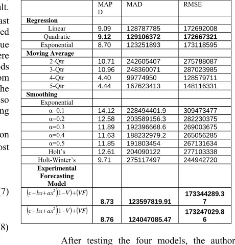
Although the error in the new equation has a higher forecast error in all three measures of error used(MAPD, MAD, and RMSE), the error produced by the experimental forecasting model (

(

c+bx+ax2

)

(

1−V

) ( )

+ VF _{) is still lower than of the}

existing forecasting technique used, therefore the experimental forecasting model still gives a more satisfactory result than the existing.

Table IV: Comparison of Forecast error by the existing techniques and by the Experimental Forecasting Model

MAP

D MAD RMSE

Regression

Linear 9.09 128787785 172692008

Quadratic 9.12 129106372 172667321

Exponential 8.70 123251893 173118595

Moving Average

2-Qtr 10.71 242605407 275788087

3-Qtr 10.96 248360071 287023985

4-Qtr 4.40 99774950 128579711

5-Qtr 4.44 167623413 148116331

Smoothing

Exponential

α=0.1 14.12 228494401.9 309473477

α=0.2 12.58 203589156.3 282230375

α=0.3 11.89 192396668.6 269003675

α=0.4 11.63 188232979.2 265056285

α=0.5 11.85 191803454 267131634

Holt’s 12.61 204090122 277103338

Holt-Winter’s 9.71 275117497 244942720

Experimental Forecasting

Model (c+bx+ax2)(1−V) ( )+VF

8.73 123597819.91

173344289.3 7

(c+bx+ax2)(1−V) ( )+VF

8.76 124047085.47

173247029.8 6

[image:5.612.288.518.444.684.2]

it only reflects the value in the 8 period, which is the 4th _{quarter of the second year. Then in the second}

model although there were improvement, it reflected the values same as what was reflected in the quadratic regression model. And lastly in the fourth model, there seems to be a trend produced which was dependent on the last few forecast values, as the values for the last few forecast increases the value for the next following period also increases, the same is true with the decrease in forecast values.

Based from the results generated from the testing of the different model formulated, the author was able to use the weight to improve an existing forecasting model, with satisfactory results, the author only regrets, the he was not able to apply the same principle to other existing forecasting model, to see if the result would be the same.

4. CONCLUSION

In the results produced by the experimental forecasting model, the error was reduced meeting the objective of this research and this resulted in the experimental forecasting model as a possible tool for forecasting. Also the multiplier used in the model had some potential of being a universal multiplier to all forecasting techniques, but this was only based on the results generated. Still it has a long way to go, as of now this research only focuses on the multiplier as part of a formulated forecasting model, and as a possible universal multiplier. With enough resources and time, this research can widen its scope to formulate a multiplier to improve forecast values and lessen the error present in the existing techniques.

5. RECOMMENDATION

Based on the results presented, gathered and analyzed, the number of sample, company, should be increased in order to have a wider understanding of the behavior of the forecast pattern. The present behavior of the forecast was limited to the point that it only repeated itself even if the actual values are not repeating itself. There was a pattern but the forecast just repeated the pattern even though, the actual does not. So there is a problem with either the technique or data. What has been used may not be enough to generate or simulate a real forecast behavior. As a recommendation, using the other forecasting technique that has not been used in this research, like ARIMA, ARMA, and Multiple Regression Method, can also be used so that the research can have a wider scope over that different forecasting techniques and models. Using more techniques or models will help in the better understanding of the different techniques and how they are use, their limitations when using them and when to use them. Knowing the different techniques will aid further researcher in identifying

the other causes of error. If the technique used does not fit the data or vise versa, will there be an increase or decrease in the presence of error in the forecasted values? And if this is the case, will that add to the error in the forecast, and does that mean there is something wrong with the technique or the data just do not fit the technique? Next is to use the multiplier in other forecasting techniques to see if the effect would be the same or would give a different result. And lastly to further test the reliability of the model, the author recommends that Kruskal-Wallis test as a reliability test should be used.

 

REFERENCES

[1] Bernard W. Taylor III Introduction to Management Science

Fifth Edition, New Jersey: Prentice-Hall, Inc., 1996. [2] Cliff T. Ragsdale Spreadsheet Modeling and Decision Analysis,

Third Edition. Cincinnati, Ohio: South-Western College Publishing, 2001.

[3] David R. Anderson, Dennis J. Sweeney and Thomas A. Williams. An Introduction To Management Science Quantitative Approaches To Decision Making Eight Edition, 1997. [4] David S. Moore Statistics Concepts and Controversies Second

Edition. New York: W.H. Freeman and Company, 1979. [5] Donald W. Fogarty, Thomas R. Huffmann and Peter W.

Stonebraker. Production and Operations Management

Cincinnati Ohio: South Western Publishing Co., 1989. [6] Douglas C. Montgomery Design and Analysis of Experiments

Fifth Edition. New York: John Wiley & Sons, Inc. 2001.

[7] Francis J. Clauss. Applied Management Science and Spreadsheet Modeling, Wadsworth Publishing Company, 1996. [8] Frederick S. Hillier and Gerald J. Lieberman. Introduction to

Operations Research Sixth Edition, 1995.

[9] Hamdy A. Taha . Operations Research: An Introduction International Edition. New Jersey: Prentice-Hall, Inc., 2001. [10] James L. Kenkel. Introductory Statistics for Management and

Economics Fourth Edition, Wadsworth Publishing Company, 1996.

[11] Richard I. Levin, David S. Rubin, Joel P. Stinson and Everette S. Gardner Jr. Quatitative Approaches to Management. Eight Edition, McGrawhill, Inc., 1992.

[12] Roberta S. Russel and Bernard W. Taylor III. perations Management Third Edition, 2000.

[13] Roger G. Schroeder. Operations Management Contemporary Concepts and Cases Second Edition, 1986.

[14] Ronald E. Walpole, Raymond H. Myers and Sharon L. Myers Probability and Statistics for Engineers and Scientists,

Sixth Edition. New Jersey: Prentice-Hall, Inc. 2000. [15] Spyros Makridakis, Steven C. Wheelwright and Rob J.

Hyndaman. Forecasting Methods and Applications Third Edition, 1998.