Features for Detecting Hedge Cues
Nobuyuki Shimizu
Information Technology Center The University of Tokyo
Hiroshi Nakagawa
Information Technology Center The University of Tokyo [email protected]
Abstract
We present a sequential labeling approach to hedge cue detection submitted to the bi-ological portion of task 1 for the CoNLL-2010 shared task. Our main approach is as follows. We make use of partial syntac-tic information together with features ob-tained from the unlabeled corpus, and con-vert the task into one of sequential BIO-tagging. If a cue is found, a sentence is classified as uncertain and certain other-wise. To examine a large number of fea-ture combinations, we employ a genetic al-gorithm. While some features obtained by this method are difficult to interpret, they were shown to improve the performance of the final system.
1 Introduction
Research on automatically extracting factual in-formation from biomedical texts has become pop-ular in recent years. Since these texts are abundant with hypotheses postulated by researchers, one hurdle that an information extraction system must overcome is to be able to determine whether or not the information is part of a hypothesis or a factual statement. Thus, detecting hedge cues that indi-cate the uncertainty of the statement is an impor-tant subtask of information extraction (IE). Hedge cues include words such as “may”, “might”, “ap-pear”, “suggest”, “putative” and “or”. They also includes phrases such as “. . .raising an intriguing question that. . .” As these expressions are sparsely scattered throughout the texts, it is not easy to gen-eralize results of machine learning from a training set to a test set. Furthermore, simply finding the expressions listed above does not guarantee that a sentence contains a hedge. Their function as a hedge cue depends on the surrounding context.
The primary objective of the CoNLL-2010 shared task (Farkas et al., 2010) is to detect hedge
cues and their scopes as are present in biomedi-cal texts. In this paper, we focus on the biologibiomedi-cal portion of task 1, and present a sequential labeling approach to hedge cue detection. The following summarizes the steps we took to achieve this goal. Similarly to previous work in hedge cue detec-tion (Morante and Daelemans, 2009), we first con-vert the task into a sequential labeling task based on the BIO scheme, where each word in a hedge cue is labeled as B-CUE, I-CUE, or O, indicating respectively the labeled word is at the beginning of a cue, inside of a cue, or outside of a hedge cue; this is similar to the tagging scheme from the CoNLL-2001 shared task. We then prepared features, and fed the training data to a sequential labeling system, a discriminative Markov model much like Conditional Random Fields (CRF), with the difference being that the model parameters are tuned using Bayes Point Machines (BPM), and then compared our model against an equivalent CRF model. To convert the result of sequential labeling to sentence classification, we simply used the presence of a hedge cue, i.e. if a cue is found, a sentence is classified as uncertain and certain oth-erwise.
To prepare features, we ran the GENIA tag-ger to add partial syntactic parse and named en-tity information. We also applied Porter’s stem-mer (Jones and Willet, 1997) to each word in the corpus. For each stem, we acquired the distribu-tion of surrounding words from the unlabeled cor-pus, and calculated the similarity between these distributions and the distribution of hedge cues in the training corpus. Given a stem and its similari-ties to different hedge cues, we took the maximum similarity and discretized it. All these features are passed on to a sequential labeling system. Using these base features, we then evaluated the effects of feature combinations by repeatedly training the system and selecting feature combinations that in-creased the performance on a heldout set. To
tomate this process, we employed a genetic algo-rithm.
The contribution of this paper is two-fold. First, we describe our system, outlined above, that we submitted to the CoNLL-2010 shared task in more detail. Second, we analyze the effects of partic-ular choices we made when building our system, especially the feature combinations and learning methods.
The rest of this paper is organized as follows. In Section 2, we detail how the task of sequential labeling is formalized in terms of linear classifi-cation, and explain the Viterbi algorithm required for prediction. We next present several algorithms for optimizing the weight vector in a linear classi-fier in Section 3. We then detail the complete list of feature templates we used for the task of hedge cue detection in Section 4. In order to evaluate the effects of feature templates, in Section 5, we re-move each feature template and find that several feature templates overfit the training set. We fi-nally conclude with Section 6.
2 Sequential Labeling
We discriminatively train a Markov model us-ing Bayes Point Machines (BPM). We will first explain linear classification, and then apply a Markov assumption to the classification formal-ism. Then we will move on to BPM. Note that we assume all features are binary in this and up-coming sections as it is sufficient for the task at hand.
In the setting of sequential labeling, given the input sequence x = (x1, x2, x3, ...xn), a system
is asked to produce the output sequence y = (y1, y2, y3, ...yn). Considering that y is a class,
sequential labeling is simply a classification with a very large number of classes. Assuming that the problem is one of linear classification, we may cre-ate a binary feature vectorφ(x)for an inputxand have a weight vector wy of the same dimension
for each classy. We choose a classythat has the highest dot product between the input vector and the weight vector for the classy. For binary classi-fication, this process is very simple: compare two dot product values. Learning is therefore reduced to specifying the weight vectors.
To follow the standard notations in sequential labeling, let weight vectors wy be stacked into
one large vector w, and let φ(x,y) be a binary feature vector such that w>φ(x,y) is equal to
w>
yφ(x). Classification is to choosey such that
y=argmaxy0(w>φ(x,y0)).
Unfortunately, a large number of classes created out of sequences makes the problem intractable, so the Markov assumption factorizesyinto a se-quence of labels, such that a label yi is affected only by the label before and after it (yi−1andyi+1
respectively) in the sequence. Each structure, or label y is now associated with a set of the parts parts(y)such thatycan be recomposed from the parts. In the case of sequential labeling, parts con-sist of statesyiand transitionsyi →yi+1between
neighboring labels. We assume that the feature vector for an entire structure y decomposes into a sum over feature vectors for individual parts as follows:φ(x,y) =Pr∈parts(y)φ(x, r). Note that we have overloaded the symbolφto apply to either a structureyor its partsr.
The Markov assumption for factoring labels lets us use the Viterbi algorithm (much like a Hidden Markov Model) in order to find
y =argmaxy0 (w>φ(x,y0))
=argmaxy0 (Pnj=1w>φ(x, y0j)
+Pnj=1−1w>φ(x, y0j→yj0+1)).
3 Optimization
We now turn to the optimization of the weight pa-rameterw. We compare three approaches – Per-ceptron, Bayes Point Machines and Conditional Random Fields, using our c++ library for struc-tured output prediction1.
Perceptron is an online update scheme that leaves the weights unchanged when the predicted output matches the target, and changes them when it does not. The update is:
wk:=wk−φ(xi,y) +φ(xi,yi).
Despite its seemingly simple update scheme, per-ceptron is known for its effectiveness and perfor-mance (Collins, 2002).
Conditional Random Fields (CRF) is a condi-tional model
P(y|x) = 1 Zx
exp(w>φ(x,y))
wherewis the weight for each feature andZxis a
normalization constant for eachx.
Zx=
X
y
exp(w>φ(x,y))
for structured output prediction. To fit the weight vectorwusing the training set {(xi,yi)}n
i=1, we
use a standard gradient-descent method to find the weight vector that maximizes the log likelihood
Pn
i logP(yi|xi) (Sha and Pereira, 2003). To avoid overfitting, the log likelihood is often pe-nalized with a spherical Gaussian weight prior:
Pn
i logP(yi|xi)− C||2w||. We also evaluated this
penalized version, varying the trade-off parameter C.
Bayes Point Machines (BPM) for structured prediction (Corston-Oliver et al., 2006) is an en-semble learning algorithm that attempts to set the weight w to be the Bayes Point which approxi-mates to Bayesian inference for linear classifiers. Assuming a uniform prior distribution overw, we revise our belief ofwafter observing the training data and produce a posterior distribution. We cre-ate the finalwbpmfor classification using a poste-rior distribution as follows:
wbpm =Ep(w|D)[w] =
|VX(D)|
i=1
p(wi|D)wi
wherep(w|D) is the posterior distribution of the weights given the dataD andEp(w|D) is the
ex-pectation taken with respect to this distribution. V(D) is the version space, which is the set of weightswithat classify the training data correctly, and |V(D)| is the size of the version space. In practice, to explore the version space of weights consistent with the training data, BPM trains a few different perceptrons (Collins, 2002) by shuffling the samples. The approximation of Bayes Point wbpmis the average of these perceptron weights:
wbpm=Ep(w|D)[w]≈
K
X
k=1
1 Kwk.
The pseudocode of the algorithm is shown in Al-gorithm 3.1. We see that the inner loop is simply a perceptron algorithm.
4 Features
4.1 Base Features
For each sentence x, we have state features, rep-resented by a binary vectorφ(x, yj0)and transition features, again a binary vectorφ(x, y0j →y0j+1).
For transition features, we do not utilize lexical-ized features. Thus, each dimension ofφ(x, y0j →
Algorithm
3.1: BPM(K, T,{(xi,yi)}n i=1)
wbpm:=0;
fork:= 1toK
Randomly shuffle the sequential order of samples{(xi,yi)}n
i=1
wk:=0;
fort:= 1toT # Perceptron iterations
fori:= 1ton # Iterate shuffled samples y:=argmaxy0(wk>φ(xi,y0))
if(y6=yi)
wk:=wk−φ(xi,y) +φ(xi,yi); wbpm:=wbpm+K1wk;
return(wbpm)
yj0+1) is an indicator function that tests a com-bination of labels, for example, O→CUE, B-CUE→I-CUE or I-CUE→O.
For state features φ(x, y0j), the indicator func-tion for each dimension tests a combinafunc-tion of yj0 and lexical features obtained from x = (x1, x2, x3, ...xn). We now list the base lexical
features that were considered for this experiment.
F0 a token, which is usually a word. As a part of preprocessing, words in each input sentence are tokenized using the GENIA tagger2. This
tokenization coincides with Penn Treebank style tokenization3.
We add a subscript to indicate the position. Fj0is exactly the input tokenxj. Fromxj, we also create other lexical features such asF1
j,Fj2,Fj3, and so on.
F1 the token in lower case, with digits replaced
by the symbol #.
F2 1 if the letters in the token are all capitalized, 0 otherwise.
F3 1 if the token contains a digit, 0 otherwise.
F4 1 if the token contains an uppercase letter, 0 otherwise.
F5 1 if the token contains a hyphen, 0 otherwise.
2Available at: http:// www-tsujii.is.s.u-tokyo.ac.jp/
GE-NIA/ tagger/
3A tokenizer is available at: http:// www.cis.upenn.edu/
F6 first letter in the token.
F7 first two letters in the token.
F8 first three letters in the token.
F9 last letter in the token.
F10 last two letters in the token.
F11 last three letters in the token.
The featuresF0 toF11are known to be useful for POS tagging. We postulated that since most frequent hedge cues tend not to be nouns, these features might help identify them.
The following three features are obtained by running the GENIA tagger.
F12 a part of speech.
F13 a CoNLL-2000 style shallow parse. For
ex-ample, B-NP or I-NP indicates that the token is a part of a base noun phrase, B-VP or I-VP indicates that it is part of a verb phrase.
F14 named entity, especially a protein name.
F15 a word stem by Porter’s stemmer4. Porter’s stemmer removes common morphological and inflectional endings from words in En-glish. It is often used as part of an informa-tion retrieval system.
Upon later inspection, it seems that Porter’s stemmer may be too aggressive in stemming words. The wordputative, for example, after be-ing processed by the stemmer, becomes simplyput
(which is clearly erroneous).
The last nine types of features utilize the unla-beled corpus for the biological portion of shared task 1, provided by the shared task organizers. For each stem, we acquire a histogram of sur-rounding words, with a window size of 3, from the unlabeled corpus. Each histogram is repre-sented as a vector; the similarity between his-tograms was then computed. The similarity met-ric we used is called the Tanimoto coefficient, also called extended/vector-based Jaccard coefficient.
vi·vj
||vi||+||vj|| −vi·vj
It is based on the dot product of two vectors and reduces to Jaccard coefficient for binary features.
4Available at: http://tartarus.org/ martin/PorterStemmer/
This metric is known to perform quite well for near-synonym discovery (Hagiwara et al., 2008). Given a stem and its similarities to different hedge cues, we took the maximum similarity and dis-cretized it.
F16 1 if similarity is bigger than 0.9, 0 otherwise.
...
F19 1 if similarity is bigger than 0.6, 0 otherwise.
...
F24 1 if similarity is bigger than 0.1, 0 otherwise.
This concludes the base features we considered.
4.2 Combinations of Base Features
In order to discover combinations of base features, we implemented a genetic algorithm (Goldberg, 1989). It is an adaptive heuristic search algorithm based on the evolutionary ideas of natural selec-tion and genetics. After splitting the training set into three partitions, given the first partition as the training set, the fitness is measured by the score of predicting the second partition. We removed the feature sets that did not score high, and intro-duced mutations – new feature sets – as replace-ments. After several generations, surviving fea-ture sets performed quite well. To avoid over fit-ting, occasionally feature sets were evaluated on the third partition, and we finally chose the feature set according to this partition.
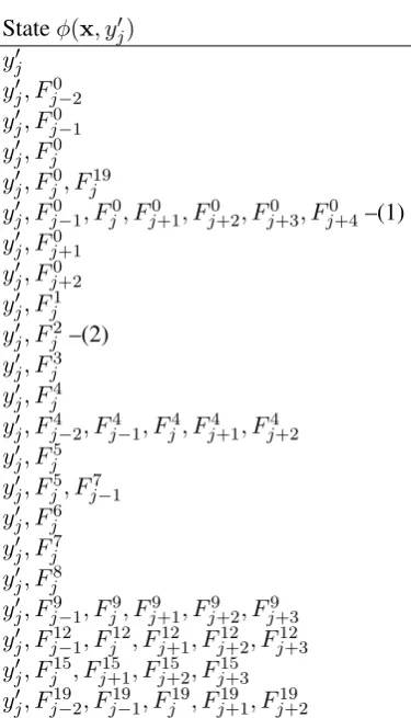
The features of the submitted system are listed in Table 1. Note that Table 1 shows the dimensions of the feature vector that evaluate to 1 givenxand yj0. The actual feature vector is created by instan-tiating all the combinations in the table using the training set.
Surprisingly, our genetic algorithm removed features F10 and F11, the last two/three let-ters in a token. It also removed the POS in-formation F12, but kept the sequence of POS
Stateφ(x, y0j) y0j
y0j, Fj0−2 y0
j, Fj0−1
y0j, F0
j y0j, F0
j, Fj19 y0j, F0
j−1, Fj0, Fj0+1, Fj0+2, Fj0+3, Fj0+4–(1)
y0j, Fj0+1 y0j, Fj0+2 y0j, Fj1 y0j, Fj2–(2) y0j, Fj3 y0j, Fj4
y0j, Fj4−2, Fj4−1, Fj4, Fj4+1, Fj4+2 y0j, F5
j y0j, F5
j, Fj7−1
y0j, F6
j y0j, F7
j y0j, Fj8
[image:5.595.88.276.56.384.2]y0j, Fj9−1, Fj9, Fj9+1, Fj9+2, Fj9+3 y0j, Fj12−1, Fj12, Fj12+1, Fj12+2, Fj12+3 y0j, Fj15, Fj15+1, Fj15+2, Fj15+3 y0j, Fj19−2, Fj19−1, Fj19, Fj19+1, Fj19+2
Table 1: Features for Sequential Labeling
5 Experiments
In order to examine the effects of learning parame-ters, we conducted experiments on the test data af-ter it was released to the participants of the shared task.
While BPM has two parameters,K andT, we fixedT = 5and variedK, the number of percep-trons. As increasing the number of perceptrons re-sults in more thorough exploration of the version space V(D), we expect that the performance of the classifier would improve asK increases. Ta-ble 2 shows how the number of perceptrons affects the performance.
T P stands for True Positive,F P for False Pos-itive, andF N for False Negative. The evaluation metrics were precisionP (the number of true
[image:5.595.77.285.676.737.2]pos-K T P F P F N P(%) R(%) F1(%) 10 641 80 149 88.90 81.14 84.84 20 644 79 146 89.07 81.52 85.13 30 644 80 146 88.95 81.52 85.07 40 645 81 145 88.84 81.65 85.09 50 645 80 145 88.97 81.65 85.15
Table 2: Effects of K in Bayes Point Machines
itives divided by the total number of elements la-beled as belonging to the positive class) recall R (the number of true positives divided by the to-tal number of elements that actually belong to the positive class) and their harmonic mean, the F1
score (F1 = 2P R/(P +R)). All figures in this
paper measure hedge cue detection performance at the sentence classification level, not word/phrase classification level. From the results, once the number of perceptrons hits 20, the performance stabilizes and does not seem to show any improve-ment.
Next, in order to examine whether or not we have overfitted to the training/heldout set, we re-moved each row of Table 1 and reevaluated the performance of the system. Reevaluation was conducted on the labeled test set released by the shared task organizers after our system’s output had been initially evaluated. Thus, these figures are comparable to the sentence classification re-sults reported in Farkas et al. (2010).
T P F P F N P(%) R(%) F1(%) 1 647 79 143 89.12 81.90 85.36 2 647 80 143 89.00 81.90 85.30 1,2 647 81 143 88.87 81.90 85.24
Table 3: Effects of removing features (1) or (2), or both
Table 3 shows the effect of removing (1), (2), or both (1) and (2), showing that they overfit the training data. Removing any other rows in Ta-ble 1 resulted in decreased classification perfor-mance. While there are other large combination features such as ones involvingF4, F9, F12, F15
andF19, we find that they do help improving the performance of the classifier. Since these fea-tures seem unintuitive to the authors, it is likely that they would not have been found without the genetic algorithm we employed. Error analysis shows that inclusion of features involvingF9
af-fects prediction of “believe”, “possible”, “puta-tive”, “assumed”, “seemed”, “if”, “presumably”, “perhaps”, “suggestion”, “suppose” and “intrigu-ing”. However, as this feature template is unfolded into a large number of features, we were unable to obtain further linguistic insights.
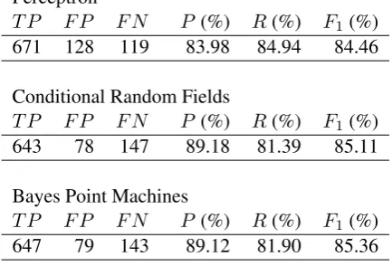
Ma-chines as we have been using. The results in Table 4 shows that BPM performs better than Percep-tron or Conditional Random Fields. As the train-ing time for BPM is better than CRF, our choice of BPM helped us to run the genetic algorithm re-peatedly as well. After several runs of empirical tuning and tweaking, the hyper-parameters of the algorithms were set as follows. Perceptron was stopped at 40 iterations (T = 40). For BPM, we fixed T = 5andK = 20. For Conditional Ran-dom Fields, we compared the penalized version withC = 1and the unpenalized version (C = 0). The results in Table 4 is that of the unpenalized version, as it performed better than the penalized version.
Perceptron
T P F P F N P (%) R(%) F1(%)
671 128 119 83.98 84.94 84.46
Conditional Random Fields
T P F P F N P (%) R(%) F1(%)
643 78 147 89.18 81.39 85.11
Bayes Point Machines
T P F P F N P (%) R(%) F1(%)
[image:6.595.73.290.282.429.2]647 79 143 89.12 81.90 85.36
Table 4: Performance of different optimization strategies
6 Conclusion
To tackle the hedge cue detection problem posed by the CoNLL-2010 shared task, we utilized a classifier for sequential labeling following previ-ous work (Morante and Daelemans, 2009). An essential part of this task is to discover the fea-tures that allow us to predict unseen hedge expres-sions. As hedge cue detection is semantic rather than syntactic in nature, useful features such as word stems tend to be specific to each word and hard to generalize. However, by using a genetic al-gorithm to examine a large number of feature com-binations, we were able to find many features with a wide context window of up to 5 words. While some features are found to overfit, our analysis shows that a number of these features are success-fully applied to the test data yielding good general-ized performance. Furthermore, we compared dif-ferent optimization schemes for structured output prediction using our c++ library, freely available
for download and use. We find that Bayes Point Machines have a good trade-off between perfor-mance and training speed, justifying our repeated usage of BPM in the genetic algorithm for feature selection.
Acknowledgments
The authors would like to thank the reviewers for their comments. This research was supported by the Information Technology Center through their grant to the first author. We would also like to thank Mr. Ono, Mr. Yonetsuji and Mr. Yamada for their contributions to the library.
References
Michael Collins. 2002. Discriminative training meth-ods for hidden Markov models: Theory and exper-iments with perceptron algorithms. InProceedings of Empirical Methods in Natural Language Process-ing (EMNLP).
Simon Corston-Oliver, Anthony Aue, Kevin Duh, and Eric Ringger. 2006. Multilingual dependency pars-ing uspars-ing bayes point machines. InProceedings of the Human Language Technology Conference of the NAACL, Main Conference, pages 160–167, June.
Rich´ard Farkas, Veronika Vincze, Gy¨orgy M´ora, J´anos Csirik, and Gy¨orgy Szarvas. 2010. The CoNLL-2010 Shared Task: Learning to Detect Hedges and their Scope in Natural Language Text. In Proceed-ings of the Fourteenth Conference on Computational Natural Language Learning (CoNLL-2010): Shared Task, pages 1–12, Uppsala, Sweden. ACL.
David E. Goldberg. 1989. Genetic Algorithms in Search, Optimization, and Machine Learning. Addison-Wesley Professional.
Masato Hagiwara, Yasuhiro Ogawa, and Katsuhiko Toyama. 2008. Context feature selection for distri-butional similarity. InProceedings of IJCNLP-08.
Karen Sp¨ark Jones and Peter Willet. 1997. Readings in Information Retrieval. Morgan Kaufmann.
Roser Morante and Walter Daelemans. 2009. Learn-ing the scope of hedge cues in biomedical texts. In BioNLP ’09: Proceedings of the Workshop on BioNLP, pages 28–36.