Technology adoption with finite horizons

Department of Economics University of Southampton Southampton SO17 1BJ UK

Discussion Papers in

Economics and Econometrics

2000

This paper is available on our website

Technology Adoption with Finite Horizons

Xavier Mateos-Planas

Department of Economics

University of Southampton

High…eld SO17 1BJ

Southampton, UK

E-Mail: [email protected]

Version 1.0

10 November 2000

Abstract

This paper analyzes the optimal sequence of technology upgrades by a …rm that lives for a …nite period of time. Other characteristics of the environment are the exis-tence of technology-speci…c learning-by-doing, technology growth, and sunk costs. A …nite planning horizon implies that the technology adoption problem is non-stationary and the frequency of adoptions changes over time. This paper provides results for the computation of the optimal plan and explores numerically the life-cycle pattern of technology switches.

1 Introduction

The adoption of technologies is an engine of economic progress. Even in the more developed economies, the resources devoted to technology adoption are substantial relative to those to technology-creating activities or research [see Jovanovic (1995)]. Di¤erent patterns of technology adoption are also invoked as part of the explanation for observed disparities in economic performances. These include economic inequalities across countries, as well as across workers [Doms et al. (1997), Bartel and Litchenberg (1987), Parente and Prescott (1994)]. Broadly viewed, decisions in many spheres of life involve elements that resemble the choice of adopting new technologies. Examples include a government considering to push ahead with policy reforms, or the decision to change a job or career by a worker. Therefore, the study of the factors that shape the patterns of the technology adoption choices is important to understand a variety of interesting choice problems.

The aim of this paper is to contribute to the analysis of technology adoption decisions in dynamic contexts. The speci…c objective of this paper is to solve and characterize the pattern of technology switches when there is a …nite time-horizon for the agent. This is a pervasive characteristic of environments where technology adoption-like decisions are made. In many labor markets workers confront a strictly …nite work-life dictated by the retirement age. Fixed-term labor contracts have a predetermined termination data. In some countries, public utilities are managed by private …rms over a predetermined period before they revert back to the government. Heads of government can be reelected only a …nite number of times. Patents typically guarantee a protection for a …nite period. The goal of the present paper is to explore the implications of this upper bound for the pattern of technology switches.

The analysis of the …nite-horizon case may also prove useful to analyze models where the time horizon is in…nite but the discount rate may change over time. The sequence of technology adoptions can be regarded as a succession of …nite-horizon problems. This feature is characteristic, for example, of dynamic general equilibrium models where the interest rate changes over the transition. Time-changing discount rates are also a feature of life-cycle models where agents of di¤erent ages face di¤erent survival probabilities.

provides the drive for switching technologies. There are costs to switching technologies though. On one hand, there is direct sunk cost associated with the upfront investment needed to implement the technology to be adopted. On the other hand, learning-by-doing on the current technology has to be foregone on adopting a new one. In this model, the process governing the emergence of new technologies and learning-by-doing are determin-istic. The key ingredient of the model is the choice by …nitely-lived agents on technology adoptions in the presence of exogenous embodied technological change and technology-speci…c learning-by-doing. This paper analyzes the choice of multiple technology adoption as a non-stationary dynamic programming problem where both the number of adoptions as well as their timing are the choice variables. The solution allows to investigate the properties of the pattern of technology adoptions under these circumstances.

The outcomes of this paper are as follows. The analysis provides an algorithm for the solution of the problem which exploits the analytical features of the model. An optimal plan may include technologies that are learned along with technologies that are replaced before learning occurs. In those cases, it is shown that the adoptions where learning occurs must necessarily take place …rst. The pattern of adoptions will in general be uneven. The qualitative and quantitative implications depend on the scope for and speed of learning-by-doing, the costs of adoption, the discount rate, and the rate of technological progress. The paper illustrates through numerical analysis the e¤ects of these factors.

There is also a body of literature on optimal investment and technology in stochas-tic models. It includes Kamien and Schwartz (1972), Jensen (1982), Balcer and Lippman (1984), McDonald and Siegel (1986), and Dixit and Pyndyck (1994). This literature empha-sizes the role of uncertainty and market structure. The present paper studies a deterministic model for a competitive agent.

The rest of the paper is organized as follows. Section 2 presents the model. Section 3 describes the decision problem and outlines the approach taken for its solution. Section 4 contains the results that characterize some properties of the optimal choice and allow its explicit computation. Section 5 demonstrates the properties of optimal plans. Section 6 concludes the paper.

2 The model

The agent lives and produces output for a period of length T. The agent is assumed to

operate a single …rm over his productive life. When the agent dies the …rm is dissolved and there is no market for discontinued …rms.

The …rm produces output using one machine. The ‡ow of output of a …rm at time

t depends on the quality of the machine in use, and on the agent’s technology-speci…c expertise. The quality of the machine is given by the technology embodied in it and I index technologies over the positive real line by a. Expertise in a technology is denoted by q. Output of a …rm that operates a machine of qualityawith technology-speci…c expertise

q is

y=q_¢a; (1)

with and a; q ₂R+. At any instant of time, a …rm may either switch to a more advanced

technology or continue to use the present one. I call technology adoption the decision to operate a new technology by replacing the current machine with another of di¤erent quality. The level of expertise on a technology evolves with its use as the result of learning-by-doing. Thus one can write q as a non-negative function q(m), where m denotes the

and Jovanovic and Nyarko (1996).

The upper bound on the technologies that can be used by the …rm at time tis denoted

by A(t). This frontier technology grows at a constant and exogenous rate ° over time.

Switching to a technologyainvolves a cost to the …rm of size¼_¢aunits of output. This …xed payment is meant to re‡ect the cost of the piece of capital that embodies the technology. This cost is a sunk cost. There is a perfect capital market where agents can borrow and lend at a constant interest rater.

The agent maximizes the present life-time value of output- net of adoption costs- from the …rm he operates. To this end, he decides which technology, among those available to him, to use at every instant over his productive life, [0; T]. The parameters that the agent

takes as given are the learning curve q(:), technological progress°, the interest rate r, and the time horizon T. The shape of q(:) will be speci…ed later. A feasible adoption plan de…nes the set of choices available to the agent.

De…nition-1 Given parameters T and the path for technology A(t) , a feasible adoption plan is de…ned by:

i. An integer number, J, denoting the number of adoptions.

ii. A sequence of real numbers_fxjg for j = 1; :::; J; J+ 1 representing the dates at which

each j-th adoption occurs, such that 0 xj < T, xj+1 > xj for j = 1; :::; J, and

xJ+1=T.

iii. A path for the …rm’s technology a(t) for t _¸ 0 such that a(t) A(t), and a(t) is

constant for t₂(xj; xj+1) allj = 1; :::; J.

The technology in Eq. (1) implies that a feasible adoption plan generates a path of outputy(t)such that, forj = 1; :::; J,

y(t) =a(xj)q(t¡xj); t2[xj; xj+1) (2)

3 The Technology Adoption Problem

value of the …rm between the initial date x and a terminal date x divided by the initial level of technology. The maximization problem of the …rm is then,

V(0; T) = max

fJ;xjg

J

X

j=1

e¡rxj_a(x

j)W(xj+1¡xj) (3)

where

W(m) _´ Z m

0 e

¡rt_q(t)dt

¡¼; (4)

and J and xj’s belong to the set of feasible adoption plans. Here W(m) is the present

value as of time 0 of output produced with a technology a= 1 over an interval of length

m, minus the cost of adopting that technology. I will make the following assumption.

Assumption 1: W(T)>0.

Assumption 2: r_¡° >0.

The …rst assumption simply means that activity has a non-negative value. The second assumption means that discounting must be su¢ciently high. Under these assumptions it is straightforward to argue that an optimal adoption plan exists where the …rst adoption takes place at time 0,x1= 0, and the adopted technology is always the frontier so a(xj) =A(xj)

all j. This results follows from the assumption that neither the relative adoption costs,

¼, nor the speed of learning, q(:), depend on the productivity of the technology to be

adopted. Therefore, if an adoption occurs at time t, the technology adopted will be the

frontier technologya(t). Thus the agent’s choice consists of deciding at every datet ₂[0; T] whether to keep on operating the current technology or switch to the frontier technology. Which technology is currently used in‡uences the time at which the next technology is introduced but has no in‡uence on the choice of which technology to adopt at that date.1 Then the solution shows that optimal technology adoption results in a sequence of dates at which the …rm switches to the frontier technology and stays there until the next upgrade. Assuming thata(0) = 1, this result allows us to rewrite the agent’s problem as

V(x1; T) = max

fJ;xjg

J

X

j=1

e¡(r¡°)xj_W(x

j+1¡xj): (5)

1_{Jovanovic and Rob (1998) also assume adoption of the frontier technology. Parente (1994), Jovanovic}

A solution must specify the timing,xj, and number, J, of adoptions. By increasing the

frequency of adoptions, the …rm is closer to the technology frontier more often. However, it has to pay adoption costs more often and reduces the bene…ts from learning. The optimal choice resolves this trade o¤. The choice of the numberJ is a novel feature of this analysis. As a benchmark for the results to come, when the horizon is in…nite and J _{! 1}then a

solution must consist of a sequence of equally spaced adoptions. The departure from this case will in general lead to a time-varying time span between consecutive adoptions.

It is useful to start by solving for the timing, taking an arbitrary J as given. The

structure of this problem is recursive: the optimal decision rule mapping xj into xj+1 for

anyj = 1;2; :::; J_¡1depends on optimal decision rules for future adoptions. Every adoption is chosen taking into account that subsequent adoptions will be decided optimally given the remaining time span. To be general, let V(x; x_jk)denote the optimal value of a …rm that lives between dates x and x, conditional on the plan containing exactly k adoptions.

Thus, ifk is optimal, then V(x; x) =V(x; x_jk), where V(:; :) is as de…ned in Eq.(5) upon lettingx1 =x andT =x. Then one can write the problem recursively as follows:

V(x; x_jk) = max

x0_2[x;x]

n

W(x0_¡x) +e¡(r¡°)(x0_¡x)

V(x0; x_jk_¡1)o: (6)

The state for this choice is given by the current date, x, and the number, k, of adoptions

contained in the plan that starts at this date. One can write the optimal choice as a policy function m(:_j:) that gives the optimal duration of use of the current adoption so

x0=x+m(x_jk).

With these pieces of notation, the problem of the agent in equation (5) can be broken down into a sequence of problems as follows.

V(xj; TjJ¡(j¡1)) = max x0_2[xj;T]

n

W(x0_¡xj) +e¡(r¡°)(x

0_¡xj)

V(x0; T_jJ_¡j)o; (7)

forj = 1; :::; J _¡1. With the convention that a plan involving zero adoptions carries zero value V(:; T_j0) = 0, it follows that V(xJ; TjJ¡(J ¡1)) =W(xJ+1¡xJ). Then the policy

functions give the optimal sequence of tenures mj =m(xjjJ¡(j¡1))andxj+1=xj +mj

Clearly this is a non-stationary dynamic programing problem for two reasons. First, the discount rate is changing over time (besides being a¤ected by the choices). Second, the value functions depend on the order of the current technology j. For the given J,

this problem could be solved backwards numerically by constructing grids for the current state. But this proves to be a highly ine¢cient procedure and provides no insight about the nature of the optimal plan. This paper will exploit the analytical properties of the problem to derive results that allow the computation of the exact optimal choices. Solving the problem involves to solve for V(x; T;J_¡(j_¡1)) for di¤erent x andj = 1; :::; J. This

recursion starts from the last-stage optimal choice,V(x; T_j1), and leads to the solution for the entire sequence V(x; T_jJ).

Of course, for the given time span T, the arbitrary number of adoptions J may be inconsistent with an optimal choice. The second part of the problem is then to …nd the optimalJ as the solution to

J = arg max

k fV(x1; Tjk) : k= 1;2:::g; (8)

The solution of the original problem in Eq. (5) is thenV(x1; T) =V(x1; TjJ).

The approach of this paper to solving the problems de…ned in equations (7) and (8) is as follows. For given J, if a solution exists to Eq. (7) it must feature

V(xj; TjJ ¡(j¡1)) =W(xj+1¡xj) +e¡(r¡°)(xj+1¡xj)V(xj+1; TjJ ¡j) (9)

forj = 1; :::; J. I will deal with situations where the value functions are di¤erentiable and the solution can be characterized as a sequence that solves a …rst-order condition. Provided that the envelope theorem holds, the above Eq. (9) implies that the optimal interior choice of xj+1 in problem (7) must satisfy

W0(xj+1¡xj)¡e¡(r¡°)(xj+1¡xj)[(r¡°)W(xj+2¡xj+1) +W0(xj+2¡xj+1)] = 0 (10)

for j = 1; :::; J _¡1. This expression has a clear interpretation in terms of the costs and bene…t of delaying the date of the next adoption. This is a 2nd order di¤erence equation in xj with initial and terminal conditions x1 = 0 and xJ+1 = T, respectively. Similarly,

Whether this condition is su¢cient to characterize a solution, or gives the only solution will depend on the assumptions underlying process of technology-speci…c skillq(:).

I will assume q(:) is a non-decreasing function of time and has an upper bound. The …rst assumption rules out depreciation of skill with time of use. The second assumption implies bounded learning which is consistent with the empirical literature like Jovanovic and Nyarko (1995), Bahk and Gort (1993), Argote and Epple (1990), and Rapping (1965). One possible speci…cation for the learning technology is the following continuous curve

q(t) = ± + (1_¡±) exp(¹t). Here ± represents the progress ratio, or the maximum factor

increase in productivity that learning can produce. On its part,¹is a measure of the speed of learning. This learning curve has been used in Parente (1994). One problem with this speci…cation is that, in general, the …rst-order condition is not su¢cient for a maximum. In other words, more that one root xj+1 to Eq.(10) may exists, possibly implying a local

minimum. This prevents the development of the approach in this paper that is based on solving the …rst-order condition. Henceforth another simpler process of learning will be considered. In particular, the following discrete-learning curve is assumed.

q(t) = 8 > < > :

1 if t < ¹

± otherwise (11)

with ± > 1. If the …rm’s experience in the use of its current technology is shorter than a period of length ¹, its level of expertise in this technology is 1. Thereafter, its level of

expertise in this technology increases to ±, which represents the progress ratio.

Even under this speci…cation, the properties of the …rst-order condition in Eq. (10) do not rule out multiple local extrema. However, a method can be developed that allows us to deal with this circumstance. The …rst step is based on solving, separately, for plans where no technology is ever learned and plans where learning occurs in all technologies. These "restricted" plans are shown to have a solution that can be characterized by applying Eq. (10) for a given number of adoptions. This will be the result in Proposition 1.

Of course, within each class of plans, a given J may not be consistent with optimality

…nding the number of adoptions may be costly. The result in Proposition 2 below allows us to determine exactly the optimal number of adoptions. To determine the optimal J, it

is possible to partition the time interval into segments. Then initial dates on the real line can be mapped into the "restricted" optimal number of adoptions using this partition.

The two previous results characterize the restricted plans. The solution to the original plan in Eq. (5) may consist of one of the restricted plans or a combination of restricted adoption plans. In the latter case, and under a fairly mild assumption, the result in proposition 3 will show that adoptions where learning takes place must occur …rst. Results are provided that allow to identify conditions where only one class of restricted plan applies throughout or, otherwise, to narrow down the region of search.

4 Optimal Adoption of Technologies

With the speci…cation of learning-by-doing in Eq. (11) above, one di¢culty is that, in general, one has to account for the possibility that learning may not occur on some tech-nologies that are adopted. Due to the discontinuity in the derivative of W(:; :), there may

be multiple local extrema at each stage of recursion in Eq. (7). Therefore, to characterize a solution it proves useful to consider two classes of restricted adoptions plans separately: plans that feature tenures shorter than¹ only, which I callS-plans, and plans that feature tenures longer than ¹only, L-plans. The restricted return functions, value functions and

adoptions plans will be indexed byv =L; S accordingly asWv_{(:; :),V}v_{(:; :),m}v

j and xvj. In

particular, given the de…nition in (4), the present value within a technology over an interval

m can be written

Wv(m) = 8 > < > :

1

r[1¡e¡

rm_{]¡¼ if v=S}

1

r[1 + (±¡1)e¡ r¹

¡±e¡rm]_¡¼ if v=L (12)

4.1 Characterization of restricted optimal plans

The optimal v-plan must satisfy a simple set of …rst order conditions. Notation is greatly simpli…ed by de…ning,

¡v(m; m0)_´I1¡e°m

r_¡°

r (I2¡r ¼ h) +I3

° re

¡rm0¸

;

with

(I1; I2; I3) =

8 > < > :

(1;1;1) if v=S

(±;1 + (±_¡1)e¡r¹_{; ±) if v=L} (13)

The following proposition is proved in appendix A.

Proposition 1. Suppose that xv

j is the jth adoption in an optimal v-plan that

ends at x. Then the continuation optimal v-plan over [xv

j; x],fxvj; xvj+1; :::; xvJg,

is unique and must satisfy the sequence of …rst order conditions

¡v(mv_i; mv_i+1) = 0; for j=J _¡1; :::; j; (14)

and

J

X

i=j

mv

i =x¡xvj; (15)

with xv

j+1=xvi +mvi = for i=j; :::; J¡1 and mvJ =x¡xvJ.

The interpretation of this result is that under a particular class of adoptions,v _{2 f}L; S_g,

the solution can be found by simply applying the mapping¡v_{(:; :) = 0 recursively as in Eq.}

(14). The restricted solution to the problem in (7) is given when j = 1 and xv

1 = 0. Here

e¡rm_¡v_{(m; m}0_{) is shorthand notation for the …rst-order condition in Eq. (10). Uniqueness}

and existence are due to the fact that the objective is well behaved and guarantees that ¡v(:; :)is monotonic in the choice variables at each stage of the recursion in Eq. (14), and that the value functions are di¤erentiable. The proof uses induction on the fact that these properties hold forj =J_¡1. Observe that the restricted S-plan is, in fact, the unrestricted

optimal plan when there is no scope for learning [i.e. ¹ > T or± = 1.].

Proposition 1 provides an algorithm for solving the optimal v-plan restricted to the

number of adoptions being J _¡(j _¡1). Appendix B describes the practical procedure to

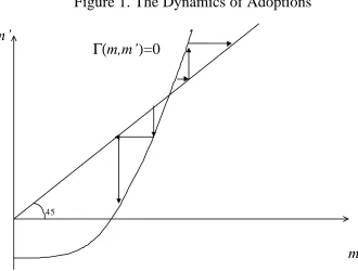
Figure 1. The Dynamics of Adoptions

m

m’

45

Γ(m,m’

)=0

Figure 1: The curve represents the optimal relation between the tenures in two consecutive adoptions.

The properties of the mapping de…ned by ¡v_{(:; :) = 0 in Eq. (14) can be analyzed. It}

is possible to show that the mapping m0 _!m is increasing and, as long as ¼ > 0, has one

…xed point which is unstable. Figure 1 shows the typical shape for this mapping. It is clear that the time pattern for tenures depends on the value of the tenure on the …rst technology relative to this …xed point. But the value of the initial tenure has to be consistent with the constraint in Eq. (15) being satis…ed after exactlyJ steps. In addition, the value ofJ that is optimal is still to be determined. This is something a priory theorizing cannot resolve.

A reference benchmark is the case where the time horizon for the problem is a multiple of the tenure length that characterizes the …xed point of this mapping. The proof of proposition 1 shows that the solution to Eq. (14) is unique [i.e. m(:_jk) is a decreasing function] so, in this case, the …xed point is a solution to the restricted problem if the time horizon contains this span of time exactly J times. From this benchmark, a reduction in J or an increase in T will then tend to increase the initial tenure length and produce an

J relative to the one that leads close to the constant pro…le for tenures. The following proposition characterizes the optimal number of adoptions.

Proposition 2. Suppose there exists an optimalv-plan over the interval[x; x], then:

(i) There exists a unique sequence _fzv

jgJj=¡1 de…ned by

Vv(zv_j; x_jJ _¡j+ 1) =Vv(zv_j; x_jJ_¡(j + 1) + 1); (16)

for j =J_¡1; J_¡2; ::: and withzv

J such that Wv(zJv; x) = 0.

(ii) x =xv

J¡k if and only ifx2(zvJ¡(k+1); zvJ¡k]and so J=k+ 1 and

Vv_{(x; x) =V}v_{(x; xjJ):}

Part (i) determines a sequence of dates where the constrained optimal value of making

k+ 1adoptions is the same as that of k adoptions [in this casek =J_¡j]]. The idea is as

follows. There is an early date such that the lifespan is long enough that making a large number of adoptions such as k+ 1 implies a higher present value than making a smaller number of adoptions such as k. However the value of makingk+ 1adoptions relative to the one fromk adoptions declines as time draws on and the time horizon becomes shorter. One can show that there is a point in time when the two values are the same, and making one less adoption produces a higher value afterwards. Therefore, such a pointzv

J¡k constitutes

an upper bound for the dates where making k+ 1adoptions can possibly be optimal. This is illustrated in …gure 2 below. Part (ii) of the proposition shows that these points zv

j are

indeed the ones that de…ne the partition on the real line that can be mapped into the optimal number of adoptions.

The procedure to solve for the optimal v-plan is thus as follows: (1) compute the

sequence ofzv

j’s as in Proposition 2-i, (2) locate the starting date and determine the number

of adoptions, J, as in Proposition 2ii, and, …nally, (3) use Proposition 1 to calculate the

timing of adoptions. Note that computing the z_jv’s in the …rst step one must already use

Figure 2. The Number of Adoptions

V(.|J-j+1)

V(.|J-(j+1)+1)

z

Figure 2: The determination of the number of adoptions.

4.2 Characterization of the optimal plan

This section shows that the previous analysis is useful to compute the solution of the (unrestricted) optimal plan. It is intuitive that the optimal (unconditional) plan over [0; T] contains some L-subinterval if ± is su¢ciently large, or ¹ or ° are su¢ciently small, or ¼

is su¢ciently large. When circumstances are the opposite, one would expect the optimal plan to contain S-subintervals. There are situations where the entire optimal plan consists of a v-plan for either v. In general, however, the optimal plan may contain L-plans and

S-plans over di¤erent periods.

Under some circumstances, the optimal plan can be shown to belong to a particular restricted class. A trivial case is that were the learning period exceeds the given lifespan or learning just cannot produce a positive value. Then only a S-plan can be optimal [this are Propositions A1 and A2i in Appendix A]. As long as an adoption with learning can produce a positive value [i.e. zL_J larger than initial date] then the optimal plan will contain

L-adoptions over some interval. If, in addition, a net positive value on a technology requires learning then the optimal plan consists of the restricted L-plan [proposition A2iia].

with the optimal plan containing both L and S plans over di¤erent intervals. In these situations, the solution procedure relies on an educated conjecture.

Assumption 3. The restricted value functionsVL_{(x; x+m) and V}S_{(x; x+m)}

do not intersect more than twice as functions ofm.

This conjecture implies that, actually, the two value functions intersect only once for a second intersection must necessarily imply a third one. The reason is that there is always a span of time long enough that learning the adopted technologies dominates [this is Lemma A4 in Appendix A]. Assumption 3 has to be made explicit because the non-linearities in the restricted value functions preclude to state it as a property. In all the calculations performed in this research this property holds. Under assumption 3, one can argue that, if the optimal plan contains both adoptions of duration longer than ¹ and adoptions of

duration shorter than ¹, then the former type of adoptions must occur …rst. Proposition 3 states this result more precisely and summarizes the discussion thus far.

Proposition 3. Assume assumption 3 above holds, then the optimal plan solves the following program,

V(0; T) = max

x?_2[0;T]

n

VL_{(0; x}?_{) +e}¡(r¡°)x?

VS_(x?_{; T)}o_{: (17)}

As a practical concern, searching for the solution without further constraints on the choice set for x? _{is highly ine¢cient. Propositions A2 to A4 in the appendix identify}

conditions for which the optimal plan is either the optimal S-plan [i.e. x? = 0] or the

optimal L-plan [i.e. x? _{=T], and, otherwise, provide results that narrow down the region}

where x?_{may lie.}

Whereas computation is feasible and e¢cient, proposition 3 cannot be used to study an-alytically the pattern of the optimal choice ofJ and the frequency of technology adoptions.

Therefore, these implications will be analyzed numerically.

5 Numerical results

section, this procedure is used to illustrate the pattern of technology adoption and assess the role of the …nite horizon. We are interested in studying the pattern of tenures over time. There are two reasons why tenures may not be constant. The …rst, already pointed in the discussion of section 4.1, is that within a restricted plan departures may be expected from the …xed point in …gure 1. The second source is the possibility that the solution contains both long adoptions with learning and short adoptions without learning. That is, x¤ in the problem of Eq. (15) above may be an interior solution. In this case, more frequent adoptions should be observed towards the end of the period.

The parametric benchmark is r = 0:065, ° = 0:02, ± = 2:0, ¹ = 0:7, ¼ = 1:12, and

T = 60. The …gures for r and ° are consistent with observations for the annual real rate

of return on equity and aggregate economic growth over long periods. A progress ratio ±

is a choice made in other studies on learning-by-doing like Klenow (1998). The speed of learning ¹is as calibrated in Mateos-Planas (forthcoming). The time horizon corresponds

to 60 years. For this setting, the optimal adoption plan features 6 adoptions and frequency increases over time asmj declines withj = 1; :::;6. This plan is the optimal L-plan. I will

analyze the e¤ect of the parameters on the adoption plan by considering departures from this benchmark setting.

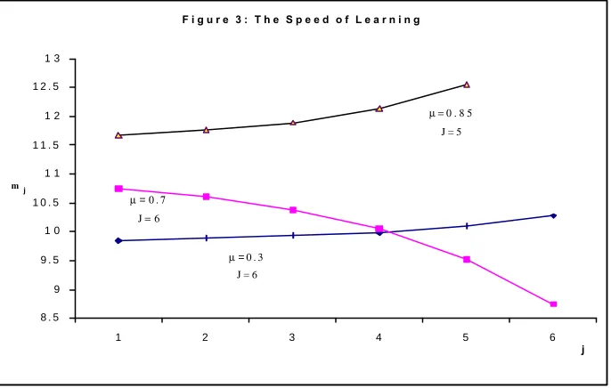
Consider …rst the parameters characterizing learning-by-doing ¹and ±. A reduction in

the speed of learning-by-doing is represented by a higher value for ¹. Graphically, such a change brings about a downward shift of the curve in …gure 1. Assume …rst that the optimal

J remains una¤ected. It should be expected that the …xed point will move to the right

relative to the value of the initial tenure, thereby tending to increase the frequency of late adoptions relative to that of early ones. The examples computed are consistent with this. In …gure 3 below, for ¹ = 0:35 the path for tenures is increasing rather than decreasing, so that, relative to the benchmark, adoptions become more frequent for earlier periods as

¹ is reduced. However, a rise in ¹ will also tend to reduce the number of adoptions J. In

this case, a higher¹can make late adoptions relatively less frequent. For example, …gure 3 also shows an increasing path for tenures associated with¹= 0:85and one less adoption.

A rise in the progress ratio±also shifts downwards the curve in …gure 1. Thus, for given

J, the slope of the time pro…le for tenures decreases and, consequently, early adoptions

become less frequent and later adoptions become more frequent. If an increase in ± also

F i g u r e 3 : T h e S p e e d o f L e a r n i n g

8 . 5 9 9 . 5 1 0 1 0 . 5 1 1 1 1 . 5 1 2 1 2 . 5 1 3

1 2 3 4 5 6

j

m_j

µ = 0 . 8 5

J = 5

µ=0 . 3

J = 6

µ=0 . 7 J= 6

Figure 3: The e¤ect of changes in¹ on the pattern of adoptions.

the e¤ect of ± on the pattern of optimal adoptions.

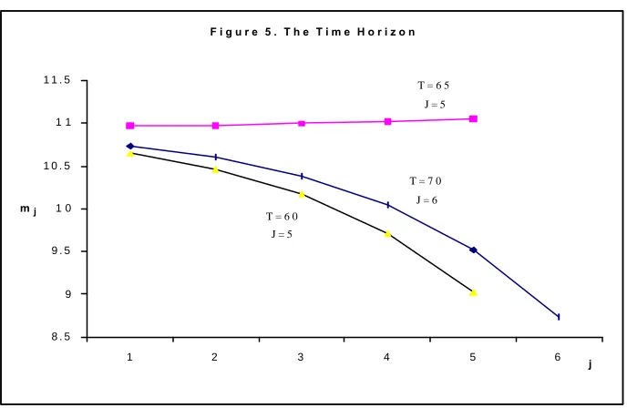
For given J, a shorter time horizon T reduces the length of the periods between

adop-tions and, according to …gure 1, tends to reduce the frequency of early adopadop-tions and increase the frequency of late adoptions. When lowerT leads to a reduction in the number

of adoptions, the e¤ect may be overturned. Figure 5 illustrates this point.

For given J, a higher interest rate r reduces the frequency of early adoptions and increase the frequency of late adoptions. When higherr leads to a reduction in the number

of adoptions, the e¤ect may be overturned. Figure 6 illustrates this point.

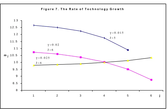
For given J, a higher rate of technical progress ° has opposite e¤ects on the timing of adoptions: frequency increases in the early adoptions. A su¢cient rise in ° makes it

optimal to adopt a larger number of technologies. Illustrative paths are shown in …gure 7 below.

For given J, the sunk cost of technology adoption, ¼, reduces the frequency of early

adoptions and increases that of late adoptions. A su¢ciently large increase in¼ leads to a smaller number of adoptions. Some illustrative …gures are displayed in …gure 8.

In the examples reported, the optimal plan is always a L-plan. However, for other parametric settings the optimal plan combines adoptions with and without learning-by-doing [for example, if ¹ = 15:0]. No example has been found that violates assumption 3

F i g u r e 4 . T h e P r o g r e s s R a t i o

8 9 1 0 1 1 1 2 1 3 1 4

1 2 3 4 5 6 j

m_j

δ=1 . 8

J = 5

δ=2 . 0 J = 6

δ=2 . 5

J = 6

Figure 4: The e¤ect of changes in± on the pattern of adoptions.

F i g u r e 5 . T h e T i m e H o r i z o n

8 . 5 9 9 . 5 1 0 1 0 . 5 1 1 1 1 . 5

1 2 3 4 5 6 _j

mj

T = 6 5 J = 5

T = 7 0 J = 6 T = 6 0

J = 5

F i g u r e 6 . T h e I n t e r e s t R a t e

8 . 5 9 9 . 5 1 0 1 0 . 5 1 1 1 1 . 5 1 2 1 2 . 5 1 3 1 3 . 5

1 2 3 4 5 6 _j

m_j

r= 0 . 0 8 J = 5

r= 0 . 0 6 5

J = 6 _r

= 0 . 0 3 J = 6

Figure 6: The e¤ect of changes inr on the pattern of adoptions.

F i g u r e 7 . T h e R a t e o f T e c h n o l o g y G r o w t h

8 8 . 5 9 9 . 5 1 0 1 0 . 5 1 1 1 1 . 5 1 2 1 2 . 5 1 3

1 2 3 4 5 6 j

mj

γ= 0 . 0 1 5 J = 5

γ= 0 . 0 2 J = 6

γ= 0 . 0 2 5 J = 6

F i g u r e 8 . T h e A d o p t i o n C o s t

8 8 . 5 9 9 . 5 1 0 1 0 . 5 1 1 1 1 . 5 1 2 1 2 . 5 1 3

1 2 3 4 5 6 j

m_j

π= 1 . 1 2 J = 6

π= 1 . 5 J = 5

π= 1 . 3 J = 5

Figure 8: The e¤ect of changes in¼ on the pattern of adoptions.

this paper. In all cases, like in Klenow (1998), technology upgrading is followed by a drop of productivity.

6 Conclusion and Final Remarks.

This paper analyzes the optimal sequence of technology upgrades by a …rm that lives for a …nite period of time. Other characteristics of the environment are the existence of technology speci…c learning-by-doing, technology growth, and sunk costs of technology adoption. The …nite planning horizon implies that the problem is non-stationary and the frequency of adoptions changes over time. This paper provides results for the computation of the optimal plan.

References

[1] Argotte, L. and Epple, D. Learning curves in manufacturing. Science, 247, 1990, 920-924.

[2] Bahk, B. and Gort, M. Decomposing learning by doing in new plants. Journal of Political Economy, 101, 1993, 561-583.

[3] Balcer, Y. and Lippman, S.A. Technological Expectations and Adoption of Improved Technology. Journal of Economic Theory 34, 1984, 292-318.

[4] Bartel, Ann P. and Frank R. Litchtenberg. The comparative advantage of educated workers in implementing new technology. The Review of Economics and Statistics, 69, 1, February 1987, 1-11.

[5] Cooley, Thomas F., Jeremy Greenwood and Mehmet Yorukoglu. The replacement problem. Journal of Monetary Economics, 40, 1997, 457-499.

[6] Dixit, A.K. and Pindyck, R.R. Investment under Uncertainty, Princeton University Press, 1994.

[7] Doms, Mark, Timothy Dunne and Kenneth R. Troske, Workers, wages, and technology. Quarterly Journal of Economics, February 1997, 253-290.

[8] Greenwood, J. and Yorukoglu, M. 1974. Rochester Center for Economic Research, Working Paper No. 429, September 1996.

[9] Hendricks, L. Equipment investment and growth in developing countries. Mimeo, March 1997.

[10] Jensen, R.A. Adoption and Di¤usion of Innovations under Uncertainty. Journal of Economic Theory 27, 1982, 182-193.

[11] Jovanovic, B. and Rafael Rob. Solow vs Solow. Mimeo, September 1998.

[12] Jovanovic, Boyan. Learning and growth. NBER Working Paper No. 5383, December 1995.

[13] Jovanovic, Boyan and Yaw Nyarko. Learning-by-doing and the choice of technology. Econometrica, Vol. 64, No. 6, 1996, 1299-1310.

[14] Jovanovic, Boyan and Yaw Nyarko. A Bayesian learning model …tted to a variety of empirical learning curves. Brooking Papers of Economic Activity (Microeconomics), 1995, 245-300.

[15] Kamien, M.I. and Schwartz, N.L.. Timing of Innovations under Rivalry.Econometrica, 40, 1972, 46-60.

[16] Klenow, Peter J. Learning curves and the cyclical behavior of manufacturing industries. Review of Economic Dynamics, 1,2 , April 1998, 531-550.

[18] Mateos-Plans, Xavier. Schooling and Distortions in a Vintage Capital Model. Review of Economic Dynamics, forthcoming.

[19] Parente, Stephen L. Learning-by-Using and the Switch to Better Machines. Review of Economic Dynamics, 3, 2000, 675-703.

[20] Parente, Stephen L. Technology adoption, learning-by-doing and economic growth. Journal of Economic Theory, 63, 1994, 346-369.

[21] Parente, Stephen L. and Edward C. Prescott. Barriers to technology adoption and development. Journal of Political Economy, 102, 2, 1994, 298-321.

[22] Rapping, Leonard A. Learning and World War II production functions. Review of Economics and Statistics, 47, 1965, 81-86.

[23] Topel, Robert H. and Michael P. Ward. Job mobility and tye careers of young men. Quarterly Journal of Economics, May, 1992, 439-479.

[24] Yorukoglu, Mehmet. The information technology productivity paradox. Review of Economic Dynamics, 1,2 , April 1998, 551-592.

A Proofs of Propositions

The proof of proposition 1 uses the two following lemmas.

Lemma A1. Consider the adoption plans solvingVv_(xv

J¡1; xj2)for some v=L; S.

(i) If xv

J¡1is theJ¡1th adoption, then xvJ exists, is unique and satis…es¡v(mvJ¡1; mvJ) =

0.

(ii) mv_J¡1(:) is a decreasing continuous function.

(iii) The value function Vv(x; x_j2) is continuously di¤erentiable inx with,

dVv_(xv

J¡1; xj2)

dxv J¡1

=W₁v(xv_J¡1; xv_J) + (r_¡°)e°(xvJ¡xJv¡1)Vv(xv J; xj1):

Proof:

(i) xv

J is the solution to the problem in Eq. (7) with j = J ¡1 and T = x. Clearly,

Vv_{(x; xj1) = W}v_{(x; x) so the objective is continuous (and di¤erentiable) and the}

choice set[xv_J¡1; x] is compact. Therefore a solution exists. A solution must be inte-rior, otherwisexv

J¡1cannot be theJ¡1th adoption. The derivative of the objective is

e¡r(x¡xvJ¡1)¡v(x¡xv

J¡1; x¡x). SincemvJ =x¡xis decreasing inx,¡v(x¡xvJ¡1; x¡x)

is monotonically decreasing in x=xv

J¡1+mvJ¡1. An interior solution is given by the

unique root of ¡v(x_¡xv_J¡1; x_¡x) = 0. Clearly it must be a maximum.

(ii) Assume not. Asxv

J¡1 increases, both mvJ¡1and, by the properties of ¡(:; :), mvJ must

increase. But this violates the constraint. Continuity follows from the continuity of ¡v_{(:; :).}

(iii) Immediate using that the …rst order condition holds with equality. Q.E.D.

Lemma A2. Consider the adoption plans solving Vv_(xv

j+1; xjJ ¡(j + 1) + 1) for some

v =L; S and some integer j J_¡1. Assume that,

(i) Givenxv_j+1, the optimalxv_j+2is unique and satis…es the …rst order condition,¡v(mv_j+1; mv_j+2) = 0.

(ii) mv

j+1(:) is a decreasing continuous function.

(iii) The value function Vv_{(x; xjJ¡(j+ 1) + 1) is continuously di¤erentiable and at the}

optimum,

dVv_(xv

j+1; xjJ ¡(j+ 1) + 1)

dxv j+1

= W₁v(xv_j+1; xv_j+2) +

(r_¡°)e¡(r¡°)(xvj+2¡xvj+1)Vv(xv

j+2; xjJ ¡(j+ 2) + 1):

Then the solution of Vv_(xv

j; xjJ¡j + 1)must satisfy the analogous of (i), (ii) and (iii).

(i) xv

j+1 is the solution to the problem in Eq. (7). By assumption (iii), the objective is

continuously di¤erentiable and the choice set[xv

j; x] is compact, so a solution exists.

A solution must be interior, otherwisexv

j cannot be the jth adoption.

By assumption(iii), the derivative of the objective is

W2(xvj; xvj+1) +e¡

(r¡°)(xv j+1¡xvj)

h

W1(xvj; xvj+1) +W(xvj; xvj+1)

i

;

which can also be written as e¡r(x¡xjv)¡v(x ¡ xv

j; mvj+1(x)). By assumption (ii),

mv

j+1 is decreasing and continuous in x, so ¡v(x¡xvj; mvj+1(x)) is continuous and

monotonically decreasing in x. An interior solution is given by the unique root of ¡v_(x¡xv

j; mvj+1(x)) = 0 which is a maximum.

ii) By assumption (ii),mv

j+1is decreasing. Inspection of ¡v(:; :)concludes the proof.

iii) Immediate using that the …rst order condition holds with equality.Q.E.D.

Proof of Proposition 1. Lemma A2 says that if properties (i), (ii) and (iii) hold for

Vv

J¡k(:; :jk + 1) for some k, then they also hold for Vv(:; :jk + 2). Lemma A1 states that

these properties hold for Vv_{(:; :jk + 1) fork = 1. Induction on k then completes the proof}

by showing that the …rst order condition in(i) is satis…ed for allk.Q.E.D.

For the proof of proposition 2 some de…nitions are required. Consider plans over[x; x].

For L-plans [i.e. v = L], the latest possible date for the last adoption, xLU

J , is given by

WL(xLU_J ; x) = 0. For S-plans [i.e. v =S], xSU_J is given by WS(xSU_J ; x) = 0.

Let the sequences _fmvU

j g and fxvUj g for j =J; J ¡1; J¡2; :::de…ne upper bounds for

earlier adoptions j J. These values are found by iterations on ¡v_{(:; :): m}vU

J =x¡xUJ,

¡(mvU

J¡1; mvUJ ) = 0, mvUJ¡1=xUJ ¡xUJ¡1,¡(mJvU¡2; mvUJ¡1) = 0,mvUJ¡2=xUJ¡1¡xUJ¡2,...

Lemma A3. The expression exp_f¡(r_¡°)x_g[Vv_{(x; xjJ¡(j¡1)¡1)¡V}v_{(x; xjJ¡j+ 1)]}

is a continuous decreasing function of x.

Proof. The proof is divided in two steps. Step 1: Prove that mv

j(x) < mvj+1(x). For

j =J_¡1 it is obvious. More generally, assume that mv

j(x)< mvj+1(x). By Proposition 1,

in an optimalv-plan the following must hold:

¡(mv

j¡1(x); mvj(x+mvj¡1(x))) = 0

¡(mv_j(x); mv_j+1(x+mv_j(x))) = 0

Suppose, by way of contradiction, thatmv

j¡1(x)¸mjv(x). Then it must follow that mvj(x+

mv

j¡1(x)) > mvj+1(x+mvj(x)). Induction on Lemmas A1 and A2 shows that tenures are

non-increasing. This and the assumption made imply x+mv

j¡1(x) < x+mvj(x). But his

contradicts the assumption made. Therefore,mv

j¡1(x)< mvj(x). Induction on the fact that

mv

J¡1(x)< mvJ(x) concludes step 1.

Step 2: The value functions involved in the derivative are continuously di¤erentiable by Lemmas A1 and A.2. Using the expressions obtained there, calculate the derivative of exp_f¡(r_¡°)x_g[Vv_{(x; xjJ¡(j ¡1) + 1)¡V}v_{(x; xjJ ¡j+ 1)] as,}

e¡(r¡°)xµ_1¡ r¡°

r

¶

hqhe¡rmvj(x)¡e¡rmvj¡1(x)

i

with q= 1 if v= S, and q= ± if v = L. The inequality follows from the result in step 1. Q.E.D.

Proof of proposition 2:

(i) For any v = L; S, existence of plans implies existence of xvU

J . The proof contains

three steps. Step 1: By de…nition ofxvU_J¡1, we have that Vv(x_JvU_¡1x_jJ_¡(J_¡1) + 1)< Vv_(xvU

J¡1; xjJ¡J+ 1). From Lemma A3, expf¡(r¡°)xg[Vv(x; xjJ¡(J¡1) + 1)¡

Vv_{(x; xjJ¡J + 1)] is monotonically decreasing in x. Therefore, z}v

J¡1 < xvUJ¡1 exists.

Step 2: prove thatVv_(xvU

j ; xjJ¡j+ 1)< Vjv+1(xvUj ; xjJ¡(j+ 1) + 1) allj. Assume

thatVv_(xvU

j+1; xjJ ¡(j+ 1) + 1)< Vv(xvUj+1; xjJ ¡(j+ 2) + 1), then

Vv(xvU_j ; x_jJ_¡j + 1) = Wv(xvU_j ; xvU_j+1) +e¡(r¡°)mvUJ Vv(xvU

j+1; xjJ¡(j + 1) + 1)

< Wv(xvU_j ; xvU_j+1) +e¡(r¡°)mvUJ Vv(xvU

j+1; xjJ¡(j + 2) + 1)

max

x

n

Wv_(xvU

j ; x) +e¡(r¡°)(x¡x

v U

j )Vv(x; xjJ ¡(j+ 2) + 1)

o

= Vv(xvU_{j j}J _¡(j + 1) + 1)

Induction on the fact proved in step 1 that the property holds forj =J_¡1concludes step 2. Step 3: Becauseexp_f¡(r_¡°)x_g[Vv_{(x; xjJ¡(j¡1) + 1)¡V}v_{(x; xjJ¡j+ 1)]}

is monotonically decreasing inx, the sequence _fzv

jgexists.

(ii) Step 1: Check thatz_jv < z_jv₊₁. More speci…cally, z_jv_¡zv_{j¡1 ¸}mv_j¡1(z_jv_¡1)> 0. Suppose not: zv

j¡1+mvj¡1(zjv¡1) > zjv. Then,

Vv(z_jv_¡1; x_jJ_¡(j_¡1) + 1) = Wv_(zv

j¡1; zjv¡1+mvj¡1(zvj¡1))

+e¡(r¡°)mvj¡1(zvj¡1)Vv(zv

j¡1+mvj¡1(zvj¡1); xjJ¡j + 1)

< Wv(z_jv_¡1; z_jv_¡1+mv_j¡1(zv_j¡1)) +e¡(r¡°)mvj¡1(zvj¡1)Vv

j+1(zjv¡1+mvj¡1(zjv¡1); xjJ ¡(j + 1) + 1)

Vv(z_jv_¡1; x_jJ_¡j+ 1)

which contradicts the result in part(i) of this proposition. Step 2: Clearly, if x = xv

J¡k, x < zvJ¡k and x > zJv¡(k+1). The converse also holds,

otherwise zv

j > zjv+1 for some j. But this possibility has been ruled out in step 1.

Q.E.D.

The proof of propoasition 3 requires some intermediate results. In what follows I de…ne a v-subinterval as an interval between two adoptions in the optimal adoption plan where

it is optimal an v-plan forv=L; S.

Proposition A.1. Suppose that x_¡x < ¹. (i) If zS

J > x thenV(x; x) =VS(x; x). (ii) If

zS

J < x thenV(x; x) = 0.

Proof: Clearly, there is no room for an L-subinterval since learning never occurs. If, in addition, the net value from using just a single technology is negative (part(i)), then it is

optimal not to make any adoption at all. If the net value can be positive (part (ii)) then

the optimal plan consists of the optimal S-plan. Q.E.D.

(i) If zL

J < x: (ia) IfzJS < x thenV(x; x) = 0. (ib) IfzJS > xthen V(x; x) = VS(x; x).

(ii) If zL

J > x: (iia) If zLJ < x¡¹ then V(x; x) =VL(x; x). (iib) If zLJ > x¡¹ then the

optimal plan may involve either S-subintervals or L-subintervals or both.

Proof: In case i, any feasible L-plan must yield a negative net value, thus there can not be

an L-subinterval in any optimal plan. If, in addition, the net value from using just a single technology is negative (ia), then it is optimal not to make any adoption at all. If the net

value can be positive (ib) then the optimal plan consists of the optimal S-plan.

In case ii, there is some L-plan that gives a positive net value. If using a technology has a positive net value only after learning occurs (part (iia)) then the optimal plan is the

optimal L-plan. Otherwise (part (iib)) some S-plans exist that give a positive net value. Q.E.D.

Proposition A.3 below characterizes the solution in case(iib)of proposition A.2. Some previous results and assumption 3 are needed.

Lemma A4.Consider the restricted optimal value functionsVS_{(x; x+m)andV}L_{(x; x+m)}

for m >0. Then, if the two value functions curves intersect at two di¤erent m, then there must be a third intersection.

Proof. The …rst intersection is at m=ma with ma¸¹and VS(x; x+m)> VL(x; x+m)

for some m > ma [this follows from direct inspection of the . Assume a second intersection

occurs at m=mb, with mb> ma. Clearly, by continuity of the restricted value functions,

VL_{(x; x+m)> V}S_{(x; x+m) form 2(m}

a; mb) andVL(x; x+m)< VS(x; x+m) for some

m > mb. I want to show that in this circumstances, a third intersection valuemc > mbmust

exist. To do this, proceed in a series of steps. Step 1: For anym > mb, the S-plan includes

some adoption xS_i in (x+ma; x+mb). Suppose that xiS ´maxfxSj < x+mbg < x+ma,

so that output under S-plan is constant over (xS

i; xSi+1). Because forx 2(x+ma; x+mb)

it holds thatVL_{(x; x)> V}S_{(x; x), output on the L-plan must be larger than output from}

the S-plan at x+ma. But then, until xSi+1 > x+mb, the L-plan that sticks with the same

technology is better than the optimal S-plan. But this is a contradiction. Step 2: Let

m=ma+mb. Then (1)VL(x; xSi)> VS(x; xSi )since xSi 2(x+ma; x+mb), and (2) since

x+m_¡xS

i < mb andx+m¡xSi > ma, we have VL(xSi ; x+m)> VS(xSi; x+m). Points (1)

and (2) imply thatVL_{(x; x+m)> V}S_{(x; x+m). Step 3: Continuity of the value functions}

implies that some mc< m exists such that the two value functions intersect. Q.E.D.

Lemma A5. Suppose assumption 3 in the main text holds. If the optimal S-plan produces

a higher value than the optimal L-plan over a certain span of time, then it must be so for any shorter span of time.

Proof. AssumeVS_{(x; x)> V}L_{(x; x). If for some x}0_{< x,V}S_{(x; x}0_{)< V}L_{(x; x}0_{), since V}S_(:)

is well-de…ned there must be an intersection below x0_{. By Lemma A4, if for x > x}0 _the

inequality is reversed, there must be yet another intersection. But this negates assumption 3. Q.E.D.

Lemma A6. Assume that the optimal can include either S-subintervals or L-subintervals

Proof. Suppose not: a S-interval of length mS _{occurs before and L-interval of length m}L_.

It must necessarily be the case that VL_(x+mS_{; x)> V}S_(x+mS_{; x). But then, by Lemma}

A5, it must be that VL_(xS

j; x) > VS(xSj; x) for all xSj adoption dates occurring over the

S-interval. In particular, this holds for xS_j =x. But this leads to the contradiction that a

S-interval can not be optimal. Q.E.D.

Proof of Proposition 3: Consider solving forV(x; x). A corollary of Lemma A6 is that

V(x; x) = max

x?

n

VL(x; x?) +e¡(r¡°)(x?¡x)VS(x?; x)o; (18)

provided that in the situations in Propositions A.1 and A.2, where the optimal plan happens to be eitherv-plan, the solution x? is non-interior. Letting, as in Eq. (5), x= 0 and x=T

concludes the proof. Q.E.D.

Proposition A.3. Assume the conjecture holds. Suppose the conditions in Proposition

A.2(iib) hold. Then zJS> x¡¹ and:

(i) If zL

J¡1> x¡¹, then V(x; x) =VS(x; x).

(ii) If zS

J¡1 < x¡¹, then there must be an L-subinterval in the optimal plan and x? 2 f[max_fx_¡¹; x+¹_g; zS

J][fxgg, where x?solves the program in the proof of Proposition

3.

(iii) IfzS_J¡1> x_¡¹ andzL_J¡1< x_¡¹, then:

(iiia) If VS_{(x; x)> V}L_{(x; x) thenV(x; x) =V}S_{(x; x).}

(iiib) If VS_{(x; x)< V}L_{(x; x) then there must be an L-subinterval in the optimal plan}

and x? _{2 f[maxfx}L

j : VS(xLj; x) < VL(xjL; x)g; zSJ][ fxgg, where x? solves Eq.

(18) in the proof of Proposition 3.

Proof: It holds that WS(z_JL; x) > WL(zL_J; x) = 0 =WS(zS_J; x), where the inequality results from the assumption that x_¡zL

J < ¹, and the two equalities hold by de…nition of zvJ for

v =L; S.

(i) In any optimal L-subinterval the last adoption must occur at a distance from the ending date less than x _¡z_JL_¡1. If zL_J¡1 > x _¡¹, then the distance from the last

adoption to the end of the period is less than ¹. Thus, no L-subinterval can be

optimal for there is a S-plan featuring the same timing that yields a higher value. (ii) If zS

J¡1 < x ¡ ¹, then VS(x ¡ ¹; x) = VS(x ¡ ¹; xj1) = VL(x ¡ ¹; x), and for

any x ₂ (zS

J¡1; x¡¹) it holds that VL(x; x) > VS(x; x) = VS(x; xj1). Then, by

Lemma A5, VL_{(x; x) > V}S_{(x; x) all x < x¡¹. If x}? _{6= x, optimality requires that}

VS(x?; x) > VL(x?; x), thus x? > x_¡¹. On the other hand, since x < x_¡¹, the

optimal plan must include some L-subinterval. Thereforex? _{> x+¹.}

(iii) If zS

J¡1> x¡¹ andzLJ¡1< x¡¹, then:

(iiia) Consider …rst the case that VS_{(x; x) > V}L_{(x; x). Now suppose that there is}

some L-subinterval in the optimal plan. By Lemma A6, this subinterval is[x; x0] for some x0 x. Optimality requires thatVS_{(x; x}0_{)< V}L_{(x; x}0_{). By Lemma A5}

(iiib) IfVS_{(x; x)< V}L_{(x; x)there must necessarily be an L-subinterval in the optimal}

plan, otherwise V(x; x) = VS_{(x; x), a contradiction. By Lemma A6, we have}

that the L-subinterval must precede the S-subinterval [if the latter exists in the optimal plan]. Hence the objective of the maximization problem in the proposition.

If the optimal plan includes a S-subinterval, then optimality requires thatVS_(x?_{; x)>}

VL_(x?_{; x). Thusx}? _>maxfxL

j :VS(xLj; x)< VL(xLj; x)gIf the optimal plan does

not include a S-subinterval, thenx?=x and V(x; x) =VL(x; x). Q.E.D.

B Computing the v-plan for given

J

Given the initial date xJ¡k, and the number of adoptionsk+ 1, the algorithm to compute

the continuation v-plan is the following. Note I suppress indexesvto save notation.

1. Pick an initial value for xJ.

2. LetSJ =mJ = ¿+T ¡xJ so that@SJ=@xJ =@ mJ=@xJ =¡1.

3. Use the …rst order condition, ¡h_(m

j; mj+1) = 0, to compute mj and

@mj

@xJ

= @mj

@mj+1

@mj+1

@xJ

;

Sj =Sj+1+mj;

@Sj

@xJ

= @Sj+1

@xJ

+@mj

@xJ

;

forj =J _¡1; J_¡2; :::; J _¡k.

4. If SJ¡k +xJ¡k¡xJ is far from zero, start again in step 1 with a new xJ updated

according to

xJ =xJ ¡

SJ¡k+xJ¡k ¡xJ @SJ¡k

@xJ ¡1