Forecasting the Next Dry Cargo Shipping Depression beyond 2018

ISSN Print: 2152-7245

DOI: 10.4236/me.2019.107110 Jul. 12, 2019 1684 Modern Economy

Forecasting the Next Dry Cargo Shipping

Depression beyond 2018

Alexandros M. Goulielmos

1_{Department of Maritime Studies, Faculty of Maritime and Industrial Studies, University of Piraeus, Piraeus, Greece}

2_{Shipping Department, Business College of Athens, Athens, Greece}

Abstract

The purpose of this research was to forecast next maritime depression beyond 2018. For this we used the nonlinear forecasting method: “Radial Basis Func-tions” [1] through the computer program NLTSA [2] allowing a prediction for 20 steps ahead. Forecasting applied to a freight rate dry cargo index since 1741 [3] and to alpha1 _{coefficient. The lowest alpha predicted was 1.01 in}

2038. Stopford’s dry cargo index forecast will be at its lowest point, of 114 (100 = 1947) units, in 2034 and 2035. Three cycles forecast to last 5, 5, and 4 years (2019-2038). Thus shipping has to learn to live with cycles… and de-pressions, but perhaps it is better if knowing them in advance.

Keywords

1929-1937, 1981-1987 and 2008-2016 Shipping Depressions, Zannetos Paradox, Forecasting Shipping Depressions, V-Statistic, Hurst Exponent, Alpha Coefficient, Rescaled Range Analysis, Radial Basis Functions

1. Introduction

Shipping suffers from frequent recessions, i.e. one every twelve years (on aver-age) [3]. A shipping depression, however, is not as frequent, because it needs a serious percentage (greater or equal to 20%) of existing fleet to be laid-up (the

shut point in economics), due to lack of demand (=seaborne trade). Shipping suffered two depressions since 1947 (Stopford, 2009, p. 106 [3]): one which

1_{Alpha shows the… “fat” in the tails of a frequency distribution. The more “fat” there, the more} standard deviation goes away from ±3σ (=maximum risk under normal distribution). In Black Monday, 1987, the “Dow Jones Ind. Index” departed 22σ from mean! Alpha manifests the “Noah Effect”, revealing a potential catastrophe, like the one in December 2008. Alpha is mathematically related to Hurst exponent-H. H reveals the cycles, and the long term dependence of freight rates. How to cite this paper: Goulielmos, A.M.

(2019) Forecasting the Next Dry Cargo Shipping Depression beyond 2018. Modern Economy, 10, 1684-1712.

https://doi.org/10.4236/me.2019.107110

Received: February 22, 2019 Accepted: July 9, 2019 Published: July 12, 2019

Copyright © 2019 by author(s) and Scientific Research Publishing Inc. This work is licensed under the Creative Commons Attribution International License (CC BY 4.0).

http://creativecommons.org/licenses/by/4.0/

DOI: 10.4236/me.2019.107110 1685 Modern Economy

started insecond half of 1981; and one which started in end-2008.

Shipping suffers also from… Jokers. The Joker is an external shock such as a war (e.g. the Yom Kippur war in 1973; the Gulf war in 1990; the Iraq war in 2003; and so on), or a canal closure (e.g. the Suez Canal closed short term in 1956 and long term in 1967-1975). But the King is seaborne trade.

Alternatively, shipping is a privileged industry, because sea covers 2/3 of Earth and the dominant centers of production are far away, by sea, from the main areas of consumption (the “distance effect”). Sea transport adds spatial utility to products, and so it is necessary. In recent decades shipping became more im-portant with the participation of China (6.6% growth in real GDP in 2018; IMF

data) and India (7.3% growth): two highly populated nations of more than two

billion consumers!

Worth noting is that maritime economic literature, after World War II, did not focus on depressions, but on growth of the fleet, and on the expansion of seaborne trade, following the global economic growth achieved (1945-end-1973). But at the end of the day, few, if any, maritime economists ex-plain successfully how to pre-know the coming of a depression, its exact dura-tion and what to do in advance to protect businesses from it…

Moreover, we believe, that the dominance of oil (and of “fossil fuels”) by 2050, will end, and it will be substituted fully by gas, and other friendly sources of energy to environment. Relevant is the recent decision of EU. We believe that the world will be forced to pass on to sources of energy exclusively friendly to environment under the pressure of the high cost of physical destructions in-cluding human deaths. Shipping is and will be affected as a result of the climatic change.

The paper is structured as follows: First is a literature review followed by me-thodology. In Part I, a historical analysis of the two main shipping depressions (1929-2008) is carried out. In Part II, the last shipping depression (2009-2016) is analyzed in more depth. In Part III, we present certain reliable features of ship-ping markets. In Part IV, two chartists’ theories about forecasting secular eco-nomic and medium shipping cycles are critically presented. In Part V, we fore-cast next shipping depression. In part VI, we set an outline for further research. Finally, we conclude.

2. Aim

Our aims were to provide an anatomy of the two last dry cargo shipping depres-sions (since second half of 1981) and show a method to improve their forecast-ing. In fact, we forecast next shipping depression (2019-2038). Moreover, we aimed at revealing the method dealing with non-periodic depressions and at de-scribing a method to find-out depression’s (average) duration.

3. Literature Review

DOI: 10.4236/me.2019.107110 1686 Modern Economy

self-correction mechanism, lasting a painful, but necessary period of adjustment of ten2 _{years (or longer). “A depression is an abnormal phenomenon produced}

by the collapse of an investment bubble”… he wrote. McConville [5] argued that the 1973 shipping oil depression removed the presumption for a consistent and underlying expansion of oil trade. The dream3 _{of the endless growth in oil}

transport to meet global oil consumption was transformed suddenly into a

nightmare by the two energy crises (1975; 1979).

Mandelbrot and Hudson, (2006/2008 preface), [6] argued that conventional

economics about investment bubbles, (or shipping depressions for us), were wrong and that these are irrational deviations from norm, caused by rapacious speculators or mass greed. But they suggested that investment bubbles can be entirely rational. Kavussanos [7] did not expand on financial-credit tsunami caused by the end-2008 depression. Soros [8] [9], argued that the undisputed faith in market forces, made us blind to see crucial instabilities. The dominant paradigm, that financial economic markets tend to equilibrium, and that devia-tions are simply random, is wrong and misleading.

Goulielmos [10] tested Hampton’s hypothesis, using econometric tools, and

called apropos Hampton’s theory a “maritime technical analysis” based on the

mystery of Fibonacci4 _{numbers [11]. Stopford [3] argued that a (shipping) crisis}

removes the imbalances in Supply and Demand, and it lasts so as to achieve this. On average, a crisis takes about ten years. He argued that shipping depressions are caused by a falling demand and an increasing supply. He also [3] argued that a shipping crisis is a poker game with a dealer (=the market). The market dan-gles the prospect of riches on each turn of cards, while shipowners struggle through the dismal recessions and raise the stakes as the cash rolls-in during booms. Ship-owners bet on ships…

Engelen et al. [12] applied, the “Rescaled Range Analysis” and the

“De-trended fluctuation analysis” (due to Kantelhardt et al.[13] to LPG market. They undermined the efficient market hypothesis… Then they found three

cycles: one four years (1993-4 to 1996-97); one six years (1998-2003) and also one six years (2003-2008). They argued that shipping cycles may not fully mate-rialize due to stochastic events. They stated that shipping cycles’ scaling and

multifractal5 _{results validate that freight rate forecasting is feasible; due also to}

returning phenomena of cycles of three to four years, or of long-range depen-dence, and lack of a time-variabilit…

Stiglitz [14] argued that the global depression in end-2008 showed that the state (USA), could not force markets to price riskcorrectly or to draft

regula-2_{We warn reader to ignore any such estimation!}

3_{A dream of Onassis, which came out to be true till his death!}

4_{In 1202 Leonard of Pisa (~1180-1250), (known as Fibonacci), published a book called Liber Abbaci,} (book of abacus), dealing with the calculating methods with the new arithmetic numbers coming from Arabs.

5_{There is a plethora of papers}

DOI: 10.4236/me.2019.107110 1687 Modern Economy

tions to minimize the damage caused by wrong estimates. Goulielmos and Psifia [15] showed that the tool used to measure risk by maritime economists, (i.e. standard deviation), is conservative and the risk is much higher than that pre-dicted by σ of normal distribution[16].

Anonymous (2013)6 _{investigated the cyclical properties of the annual growth}

of BDI (Baltic Dry Index) (1993-2012) using 231 months and found cycles last-ing from three to five years. The method applied was due to Harding & Pagan in 2006 and Harding in 2008, while the forecasting method was a trigonometric re-gression. Goulielmos [17] rejected the idea that ship-owners are irrational, fol-lowing an analysis based on Keynes. Moreover, he rejected [17] Hampton’s [10] argument that groups of investors, meaning also shipowners, do not, necessarily,

act rationally.

Zheng and Lan [18] applied to tankers a multifractal7 _{analysis using}

nonpa-rametric specifications to deal with nonlinear and non-stationary time series, characterized by fat-tails8 _{in probability distributions and volatility clusters.}

They used a generalization of the “de-trended fluctuation analysis” (due to Kan-telhardt et al.[13]. Their model [18] applied to 6 tanker types: VLCC (very large crude carriers); ULCC (ultra large crude carriers), Suezmax, Aframax, Panamax and Handy, using daily returns. They concluded that tanker markets are frac-tal… [19]. They used rolling windows, and found that the Hurst9 _exponent

va-ried from a minimum of 0.40 (for Handy) to a maximum of 1.00 (for Handy,

Panamax and Suezmax) and a dominance of memory… . The crude oil market

found an oligopoly10 _{of… nations ([18], p. 558) and the tanker market found}

highly competitive ([18], p. 558) [20]…

Summarizing, Koopmans [21] argued that Tinbergen was wrong in assuming

equal cycles up and down, as tanker booms were shorter, but he was also wrong, because one boom in 1988-1997 lasted 10 years (Stopford p. 106, [3]) and one in 2003-2008 lasted 5 years! Sanko Steamship Co of Japan committed a historical mistake in 1982 by investing massively in new dry cargo ships, believing in a shipping cycle of two years up and two years down (Couper, p. 37-8, [22]; Stop-ford, p. 126, [3]). Copying other shipowners is also a symptom of the inability to forecast shipping markets.

We mentioned Joker (Peters, p. 60, [23]). The Joker represents also strikes11_,

6_{“The Baltic Dry Index: Cyclical Analysis and Forecasting”; probably published in Logistics and}

Transportation Review, Part E, in 2013.

7_{Mandelbrot-Hudson’s, ([6], p. 217), model is a representation of the fractional Brownian motion of} multifractal time, or a multifractal model of Assets Returns in Brownian motion, expressed by an equation. The trading time is expressed by f(α). Its purpose is to re-distribute time. Time is short-ened and stretched… The main variable: price, becomes a function of trading time, a function of clock time; here the end is to manage wild fluctuations, and volatility, which clusters.

8_{Characteristic applicable to shipping time series as well.}

9_{Due to Hurst, indicating cycles etc. in time series. H = 0.50 stands for Random Walk, where alpha =} 2.

10_{Oligopoly of governments: i.e. those of OPEC, Russia, Venezuela etc.}

11_{In “Seatrade” (monthly shipping journal), an article about the re-opening of the Suez Canal in June}

DOI: 10.4236/me.2019.107110 1688 Modern Economy

embargos and all international events disrupting the workings of supply and demand. The post Second World War period (1947-2008) produced 9 Jokers (part VI). As argued by Peters ([23] p. 61), if a market is a Hurst process, as shipping is, it exhibits trends that persist till an economic equivalent of a Joker arises to change its bias in magnitude, in direction or in both…

In [18], the time-dependent Hurst exponent12 _{diminished as data’s frequency}

increased (over same days, weeks and months)… i.e. as the duration of data in-creased, the more random the same data became… Let us take the box representing 2048 days, (about 8 years), from [18], then daily H is 0.62, the weekly is 0.51 and the monthly is 0.43 (applying “Rescaled Range Analysis”). How the same time series are persistent in days and weeks, and anti-persistent in

months? The reverse had to be also true. The maximum H13 _{here is 0.70}

(round.), and though it varied over time, this characterized the whole time series

(Peters [23])14_{. The persistent time series is the exclusive candidates for a}

depression, and for this reason is important.

In [18] high Hs found, but low α… But alpha15 _{= 1/H. As argued by}

Mandel-brot & Hudson [6] (p. 202), H and alpha are closely interrelated forming a dual relationship (mathematically). But what is important is that economists [6][12], and ourselves, believe that if a long memory exists (H > 0.50 ≤ 1) in time series, this undercuts the efficient market hypothesis!16

4. Methodology

A robust method we used is the Rescaled Range Analysis. This is a methodology in non-parametric statistics due to Hurst [24]; (Peters [23] Mandelbrot and Hudson, (2006/2008 preface), [6]).

4.1. An Historical Account

Hurst worked extensively on a Nile River dam, as hydrologist, who undertook from UK Government to build an efficient and effective dam there ([23]; Man-delbrot & Hudson, (2006/2008), [6]; Steeb [25], p. 108). Egyptians supplied Hurst with extremely long time records, i.e. of 847 years! Hydrologists, before Hurst, assumed that the inflow of water into reservoirs was a random process. To Hurst’s surprise data did not represent a random structure, and the statistical tools indicated no correlation between various observations. Hurst developed a

12_{In methodology.}

13_{Rounded from 0.689849 for n ≥ 10 and n = 260 (278-1-9-8) years.}

14_{The longer was about 15 years. Data that last less than 20 years cannot reveal cycles of 20 years or} longer. Looking at the 5 graphs in [18], of a variable time duration of H, almost all Hs were ≥ 0.50 and ≤ 1.00 (Handy only had H = 0.40) (Oct. 2011).

15_{A coefficient indicating volatility and risk; alpha is also the measure of the “peak-ed-ness” of the}

probability density function.

16_{Exarchou-Moutafidis-Simitsis-Tzouvara and Adamidis in 2013 found (2007-2012) that the 1132}

DOI: 10.4236/me.2019.107110 1689 Modern Economy

set of new tools in statistics (mentioned below) to examine data deviating from a Gaussian distribution.

4.2. Einstein’s Contribution

Einstein [26], during his highly productive phase, did an extensive study on

Brownian motion, (stated first in 1828 by Robert Brown—a botanist, and re-mained unsolved since then): i.e. what is known as the model of random walk.

Einstein proved that the distance covered by a random particle, undergoing random collisions from all sides, is directly related to the square root of time:

R k T= _{(1), where R stands for distance, k is a constant and T is the index of}

time.

4.3. Hurst’s Contribution

Hurst [24] generalized Brownian motion to be applicable to a broader class of

timeseries: _{R S kT=} H _{(2), where R is the range of a time series, H is the}

rele-vant exponent (or power coefficient), and S is the (local) standard deviation. Equation (2) scales as time increment increases by a power law. R indicates the distance of a time series; R/S is a timeless and dimensionless ratio17 _{(rescaled by}

S). The Hurst exponent provides a criterion for three cases: if H = 1/2 = random walk = independent series (white noise). If 0 ≤ H ≤ 0.5, series is anti-persistent (pink noise) and if 0.5 < H ≤ 1, series is persistent (black noise). In Nile, H = 0.91, meaning that River’s waters indicated a speed higher than random and so previous flows influenced next, and present and future flows remembered pre-vious overflows, i.e. they have a memory. Given that H = 0.69 or 0.70 here, mari-time series, if found decreasing, is most likely to continue to fall rightly next; the reverse is also true. This phenomenon is called Joseph effect, as it indicates seven years of fortune followed by seven years of famine (Bible). Moreover, these series has only the potential of sudden catastrophes, called apropos Noah effect (Bible; names coined by Mandelbrot) as happened.

4.4. H’s Estimation

To estimate H, we take logs of (2): log

(

)

( )

( )

( )

(3)18_{, where log(T) is the independent variable, log(R/S) is the dependent}

varia-ble and log(c) is the intercept. We run regression (3) using NLTSA [2] computer program and took results for T = n ≥ 10, i.e. nine results are ignored [25], and one observation is used to get first log differences. The range (R) of a time series is the difference between its maximum and its minimum value (indicating the total distance covered by time series).

4.5. V Statistic

Given that R S V= ∗ n _{(4) and solving (4) for} V V: =

(

)

DOI: 10.4236/me.2019.107110 1690 Modern Economy

the V-statistic)19_{. The V-statistic works particularly well in the presence of noise}

(Peters, p. 92, [23]). Equation (5) gives a precise measurement of a depression’s length in calendar time. Rescaled range analysis provides a graphical method to

calculate the time, which a depression lasts (Peters, p. 92, [23]). The discontinui-ties in the plot of (V/logn) are sought. The non-periodic depressions are shown when the (V-statistic’s) plot starts to flatten-out, and its slope diminishesat the end of each depression.

4.6. The Relationship between Alpha and H

Important is that H is connected with alpha. To estimate alpha there is the orig-inal methods of Mandelbrot [27] and Fama [28]. We will follow Peters, p. 212, [23]): let the sum of a (stable) variable R, in an interval n, be: 1/

1

Rn R n₌ α _(6),

where R1 the initial value; i.e. the sum of n values of R scales by n1/α times

initial value. Taking logs: logRn=1 logα n+logR1 (7), and solving for alpha: 1

alpha log log= n Rn−logR _{(8); (8) equals 1/H, if (logRn − logR1) is replaced}

by (logR/S) given that (logR/S) = (logn)H, and so alpha 1= H _{(9). (9) gave us}

an estimated alpha coefficient for shipping time series equal to 1.43 (round.). According to Rescaled Range Analysis, H exponent determines the order of events: good years follow good ones and bad ones follow bad ones. Moreover, shipping time series produces trends and cycles. Alpha exponent measures how wildly freight rates vary and how fat the tails of the distribution of freight rates’ changes are. It is a proper tool to recognize violent freight markets.

Mandelbrot and Hudson, (2006/2008 preface) [6], argued that an economic

depression, (or a shipping depression for us), occurs if alpha = 1.00 ≤ 1.7. This level of alpha indicates that a Noah Effect, or the rapid reversal of trends, is like-ly. The Noah effect is the tendency of (a persistent) time series to produce abrupt

and discontinuous changes, or apropos for shipping depressions as in Dec. 2008.

4.7. The Bubbles

The bubbles (depressions) flow from the entwined effects of a long-term depen-dence (measured by Hurst exponent),and by a discontinuity,(measured by al-pha). This explanation (due to[6]) supports our argument that ship-owners are rational, like other investors, and more important is that we can use alpha. Fi-nancial markets and shipping ones behave the same way.

5. Part I: Analysis of Two Shipping Depressions, 1929-2008

First, we will restore optimism among shipowners.

5.1. Five Universal Truths about Shipping Markets

1) The decline in seaborne trade20 _{is the main cause of a shipping depression,}

because seaborne trade—given distances—is shipping demand (derived

de-19_{If (R/S)n versus n expresses a straight line, then data are random.}

DOI: 10.4236/me.2019.107110 1691 Modern Economy

mand). 2) The world supply of ship space cannot be coordinated, despite various programs, from time to time (e.g.: scrap 2 tons, build 1). 3) Shipping supply is in the hands of about 30,000 shipping companies, the majority of which are small, owning three vessels (on average). The ships are managed mostly by private, in-dependent, managers. 4) Global demand for ship space is in the hands of those many thousands importing and exporting companies by sea. Here it matters what promotes sea trade. 5) The oversupply of ship space, relatively to demand,

is the other main cause of a shipping depression.

5.2. The Picture of about 300 Years of the Dry Cargo

Shipping Market

The picture of “shipping dry cargo market” between 1741 and 2019 (March) is as Figure 1.

As shown, three main shipping peaks occurred: in 1808-1813 (during

Na-poleonic Wars); in 1918 (end of the Great War), when almost all commercial ships destroyed; and in 2003-2008, due mainly to China’s trade. We have noticed that in 2007 demand for dry bulk carriers was intensified and was related with the imports of iron ore and steel by China (380 mt iron ore) and Japan.

5.3. The 1929-1937 Shipping Depression

In 1929 (end) the Wall Street crashed causing a shipping depression. The trade fell 26%, while world fleet… increased (1931-1934); 21% of total tonnage of world fleet (14 million GRT-gross registered tonnage) was laid up (1932), i.e. 5 times higher than the normal. A heavy scrapping took place; second hand prices fell by 50% in 1930, and further in 1933. In 1933, prices of second hand ships were called distress prices due to their low level. Five million GRT of ships

Figure 1. “Maritime economics freight index”, 1741-2019 (March). Source: data from

DOI: 10.4236/me.2019.107110 1692 Modern Economy

scrapped (7.5% of the 1932 world fleet) (1935-1937).

5.4. The 1981-1987 Depression

The dry cargo freight rates fell below operating cost (1981-1987) causing losses (Figure 2).

The sharp fall of dry cargo freight market started in 1981 (end), when a Pa-namax ship earned $8500/day in December from $14,000 in January (61% less). The Joker here was the strike of coalminers in the USA, which collapsed the

whole Atlantic market. The freight rates/day further halved to $4200

(end-1982)… Technology contributed in replacing (old) ships with ships having

fuel-saving main engines, after the serious double increases in fuel cost (1975; 1979). Bunker costs covered 41% of annual operating cost (including voyage ex-penses) by 1980 of a newly-built tanker!

5.4.2. The Laid-Up Situation

A large number of ships were laid-up (1975-1985) (Figure 3).

Figure 2. “Maritime economics freight index”, 1979-1987 (1947 = 100).

Source: Data from Stopford [3]. Colors have no particular meaning.

DOI: 10.4236/me.2019.107110 1693 Modern Economy

As shown, the laid-up tonnage peaked-up in 1982 (84 m dwt). The overall to-tal was 317 m (1981-1985), if we add the amounts corresponding to yearly peaks. This prevented the market from reaching equilibrium, causing freight rates to go up and down, till oversupply absorbed. Laid-up tonnage is a stand-by supply removed from sight, but not from fight (market)!

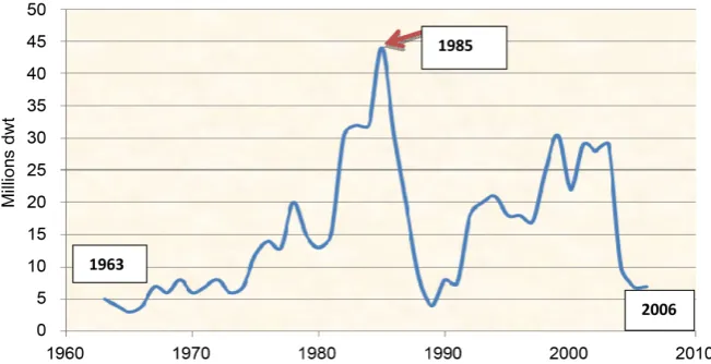
5.4.3. Scrapping

We assume that all ships with no hope of earning anything above operating costs in next three21 _{years, they end-up in scrapping yards. As shown (Figure 4) they}

reached a top, (1985), of 44 m dwt. Comparing Figure 3 with Figure 4, we see that a massive lay-up emerged first, and then—after three years—a substantial scrapping followed. Worth noting is also that scrapping (44 m peak) covered almost 1/2 of the laid-up tonnage (84 m peak). In total, 231 m tons scrapped (1979-1987).

Moreover, over 145 m dwt of tankers scrapped (1977-1985). The majority scrapped, (in 1985), concerned tankers of over 175,000 dwt each (i.e. 76%: 18.4 m dwt) (data from Asian Shipping [29]). These tankers were built with a dream in the mind of their owners of a cheap and abundant oil lasting for ever. OPEC had a different opinion.

1) Why valuable ships are scrapped?

There are six reasons: a) high age: ships scrapped are old; b) high cost: ships

scrapped had e.g. an expensive mean of propulsion (which could not be

eco-nomically replaced); in 1985 steam turbine ships had a poor economic perfor-mance; c) legal obsolescence: IMO required then the: inert gas system, crude oil washing and dedicated clean ballast tanks; d) low market: it plays an important role (economic obsolescence). In 1982, tankers had a surplus of 139 m dwt (40%) on a 349 m total supply… In 1985, dry bulks had a surplus of 48 m (21%) on a 225 m total supply; e) high scrap price: ships can earn a satisfactory price

Figure 4. Scrapping of ships, 1963-2006 (millions dwt). Source: Lloyd’s statistical tables,

various years.

21_{According to our experience. The hope of a Greek shipowner for better freight rates, needs three}

DOI: 10.4236/me.2019.107110 1694 Modern Economy

[30]; f) high scrap funds: the greater the size of ships (increased by leaps and bounds to reap economies of scale), the more serious became the funds coming from scrapping!

5.4.4. Slow Steaming etc.

Shipowners adopt various methods to reduce oversupply—for which they are… personally responsible. Ships in order to reduce fuel costs, during a depression, they steam slowly (Figure 5). Moreover, tankers can be used for storage of oil, and if cleaned-up,to carry grain!

As shown, the bulk carriers falling between 10,000 and 39,999 dwt,(more in this than in any other class), slow-steamed. They peaked in March 1982 (14 m dwt). In tankers, the greater numbers of slow-steamed ships were in sizes of 150,000 dwt and over, with a peak of 43.3 million (June 1981)… This was the revenge of… economies of scale, we may say, because shipowners ignored the golden rule: “an economy of scale is a good thing, if there is a good cargo”, i.e. enough cargo.

The surplus22 _{in tankers varied from 80 m dwt (1981) to 130 m (mid-1983)}

and 80 m (1985). The supply of tankers was 265 m dwt (end-1985) and the de-mand was only 180 m! There was a surplus of 85 m (32% of supply). This sur-plus was: slow steaming: 30 m or 35%; laid-up: 30 m or 35%; used as storage: 25 m or 30%. In bulk-carriers, the fleet was 225 m dwt (end-1985) and the demand only 175 m. The surplus was 50 m (22% of supply). Slow steaming in bulk-carriers accounted for 50% of their surplus.

5.5. The 1998-2008 Situation

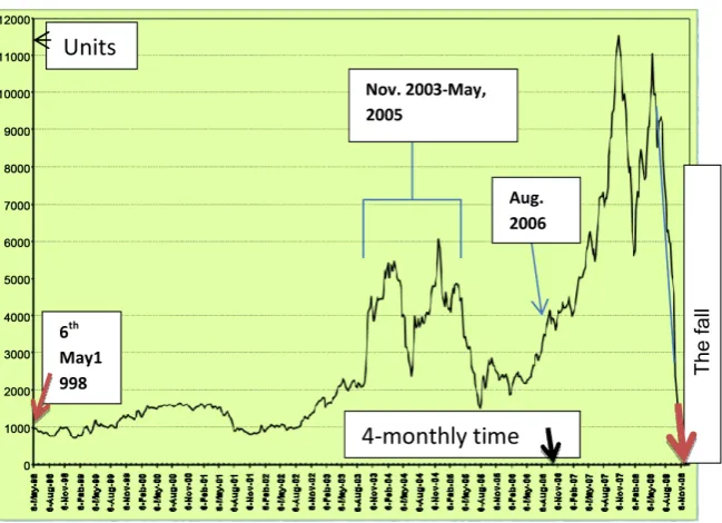
The market situation between 1998 (May) and 2008 (Nov.), 10 years prior to Global Financial Crisis, is next presented (Figure 6), as a prelude to last depression.

Figure 5. Tonnage of dry bulk carriers, in the class of 10,000 - 39,999 dwt, in

slow-steaming, 1980-1987. Source: Data from lloyd’s shipping economist (in 1989).

DOI: 10.4236/me.2019.107110 1695 Modern Economy

Figure 6. The Baltic Panamax Index (BPI) from 1998 (06/05) to 2008 (06/11) (weekly).

Source: Data from Clarkson’s.

As shown, the vertical fall in BPI in 2008 (6th _{August)—is dramatic and}

unex-pected: pushing shipowners into the 2009-2016 depression. Profitable markets emerged before this catastrophe, between 2003 (6th _{August) and 2005 (6}th

Au-gust) and exceptionally profitable from 2005 (6th _{August) to 2008 (6}th _{August) (a}

five years boom).

6. Part II: The Last Shipping Depression, 2009-2016

As shown (Figure 7), the orders for dry cargo ships fell to 50 m dwt

(end-2008-2013). This fall started in 2010, and continued in 2013, (in 2013 or-ders were 50 m dwt, i.e. 6% of existing fleet), and beyond. Our question was as to why orders did not stop completely… as one would expect during a depression? As shown, the peak in deliveries appeared four years after the peak in orders. Ship-owners in a depression, try to postpone deliveries… and cancel as many orders as possible. Shipyards, however, recorded large orders between 2009 and 2012. Dry cargo ships delivered to owners, between 2009 and 2013, were excep-tional many and varied from 7.5% (2009) to 16% (2012) of existing fleet. Orders increased, and as a result deliveries increased… though not equally. The con-struction time is a flexible variable depending on the intensity of demand and the availability of berths. This manifested that the cause of shipowners to order was the amount of revenue entered into companies’ vaults, and not the crisis flowing around due to GFC.

Scrapping is the only equilibrating mechanism between demand and supply; it reached 100 m dwt between 2009 and 2013, i.e. between 2% and 5% of existing fleet (Figure 8).

DOI: 10.4236/me.2019.107110 1696 Modern Economy

Figure 7. Deliveries and orders of dry cargo ships, 2009-2013, (millions dwt). Source:

Data from J. Grieg & Co [32].

Figure 8. Deliveries and scrapping, 1963-2006. Source: Data from UNCTAD-various

years.

surplus tonnage quickly (exception: the period mid-1981-mid-1987). Scrapping removed only 1/3 of the tonnage delivered. Thus a market based on scrapping for its improvement needs time (three years), given demand.

Deliveries (1963-1982) surpassed scrapping by 50 m dwt (max.) during most of this period. Scrapping intensified (during the depression) from 1981 to 1987. Scrapping fell by an almost steady amount of 10 m dwt/year below deliveries (1988-2003: 15 years). The gap between deliveries and scrapping widened sharp-ly in 2006 to 70 m dwt. A strong demand reduces scrapping and magnifies deli-veries in a serious level.

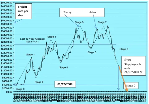
Figure 9 presents the situation in the freight rate market from 2008 to 2010.

As shown, a short-term shipping cycle (3 - 4 years) unfolds in 8 stages, lasting from 2008 to 2010 (31 months) (instead of 36 theoretically). Freight rates varied from $4000 to $39,000, but they had to return to $4000 according to theory (2010; 12/09).

DOI: 10.4236/me.2019.107110 1697 Modern Economy

Figure 9. Short term shipping cycle of four time charters on baltic routes (Panamax) 2008 (1st _{Dec.)-2010 (24}th _{July). Source: Data}

from Clarkson’s; mimic Hampton’s cycle; modified from that designed by my student Psifia.

Table 1. BDI 2010-2018.

Year BDI Year BDI

2010 $4200 2011 $~2000

2012 (*) $~1,000 647 units = collapse of the

index (**) 2015 end 504 units

2016 (April); We reckon 2016 to be the end of the 2009 depression

(which lasted 8 years). 500 units (lowest) 2017 May 994 units

2018 1,109 units (*) A gloomy year with record deliveries, dismal earnings and record scrapping

(**) Though seaborne trade increased by ~4% in 2011 and ~6% in 2012

Source: author from various publications.

7. Part III: Common Features of Shipping Markets

7.1. The over Ordering of Ships

psycho-DOI: 10.4236/me.2019.107110 1698 Modern Economy

logical law, i.e. the hope of shipowners for a better day. But the 1979-1991 tanker depression took more than 13 years for the market to absorb the large surplus of some 100 m dwt mainly via scrapping [4]!

7.2. Depression Reserves/Lay-Up

At the end of a depression, companies have to build-up “depression reserves” to cope with next one, which is expected with a high degree of certainty (our opi-nion). Moreover, ship-owners should not charter ships at all in a very bad mar-ket, but better lay-them-up [4][33].

7.3. Two Secrets of Shipping Management

Figure 10 indicates that the successful management of a shipping company must

take 2 essential facts into account.

Part (a) shows that the change in shipping net revenue (1986-2007), (net of operating costs), varied from $1 m (1986) to $16.5 m (2007)! In 2007, annual revenue was greater than the 1/3 of the value of the vessel (part b). Moreover,

buying a ship in 1986, at $13.5 m, and selling her in 2007, at $48 m, one gained $34.5 m… So, one good sale of a ship is equivalent to three-four years of (net)

profit from operations.

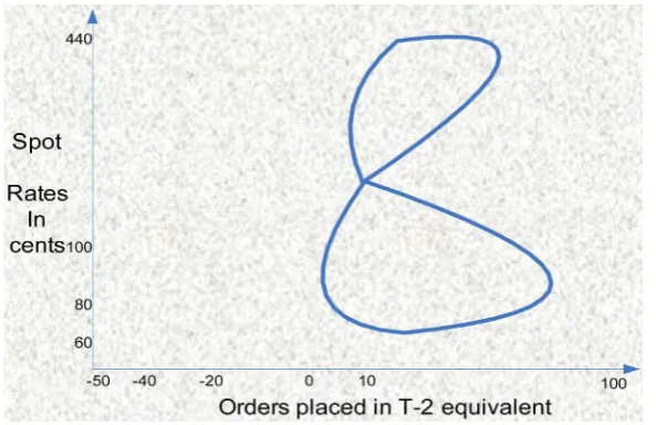
7.4. Zannetos’ Paradox

Zannetos [34] saw the abrupt changes occurring in tanker ship-owners’ expecta-tions, varying from elastic to inelastic, and back to elastic, in relation to orders placed and monthly spot rates (1949-1958). He was surprised. He argued that operators have definitely… lost their memory. A sketch (Figure 11) shows the scatter of monthly rates and the orders placed to move in a loop pattern resem-bling number 8.

Zannetos’ paradox is still valid today as shown by the time charter rates in force in 1999-2009 (Figure 12).

Figure 10. (a) Net revenue for grain (US Gulf-Rotterdam); (b) Values of ships

DOI: 10.4236/me.2019.107110 1699 Modern Economy

Figure 11. Orders placed against the index of spot rates, 1949-1953 (Monthly).

Source: Idea from Zannetos [34].

Figure 12. Monthly time charters for Cape23 _{ships and the number of ships ordered, 1999}

(April)-2009 (Nov).

As shown, the orders of ships moved closely with monthly time charters, with a lag of 6 months (read from figure). Orders stopped from 2008 (Nov.) to 2009 (July), but re-started during 2009 (second half), when time charter rates reached $80,000/month! Keynes [17] argued that the current price, i.e. the spot freight rate for shipping, influences expectations about an investment, but he insisted that this is not the exclusive, or even the dominant, cause. So, time charters, as shown, by having an amount of long-term expectations in them… are the do-23_{A Cape transports bulk cargoes, but is too wide to transit Panama Canal; she travels via Cape,}

DOI: 10.4236/me.2019.107110 1700 Modern Economy minant cause, confirming Keynes.

Under depressed freight rates (end-1982), a large number of orders placed, first by Japanese, and then by Greeks, Norwegians and others, reaching a total of 32 m dwt! These orders initiated by the “Sanko Steamship Company of Japan”, which secretly ordered 123 dry cargo ships of a total of 4.5 million dwt [3][4] [11][22]! The key-idea24 _{was to order (dry cargo) ships at the end of 1982,}

ex-pecting depression to last two years, i.e. till end-1984. So, ships’ delivery would coincide with the next upturn of the market, expected to be in January 1985, (a genius idea)… but market improved 2.5 years later25_…

Symmetry in the period of a depression is rooted in ancient Greeks, who as-sumed circle to be the divine shape. Moreover, Greeks believed that the Sun moves round the Earth in a circle… In the Fourier analysis, the irregularly shaped time series are the sum of a number of periodic sine waves, each with different frequencies and amplitudes. Spectral analysis attempted to break an observed irregular time series, with no obvious pattern, into sine waves, and impose an unobserved periodic structure on the observed non-periodic time se-ries [23]…

8. Part IV: Chartists’ Theories of Secular Economic and

Medium Term Shipping Cycles

8.1. Long Waves, 1734-2058

Goulielmos [35] warned: Be careful during the 2004 global shipping fair

Poseidonia26_{, because a world depression is coming, similar to that of 1929-1937.}

This statement based on the “theory of long waves”, advanced first by the

Rus-sian economist Kondratieff (in 1926 in German; and in 1935 in English) [36]

[37], (Figure 13).

As shown, the world economy passed through 5 lows: 1788, 1842, 1896, 1950, and 2004 (2008 really), and it will pass another one at 2058. The symmetry of the waves is apparent27_{. By 2031 (2004 + 27 years) world economy is expected to}

reach a new high.

8.2. Shipping Chartists’ Medium-Term Recessions (16 - 24 Years)

Hampton [38][39] argued that shipping exhibits a (long) recession cycle of 16 - 24 years, unfolding in two equal phases: a building-up phase and a correction phase (Figure 14). Again this model adopts symmetry.

As shown, freight rates form six pyramids, over two equal chronological phases, unfolding from zero time (to 8 years) or to 12 years and from 12 years

24_{To order ships and buy used ones (younger, larger and dispose thereafter the smaller, older) is the} Greek investment policy, at rock bottom prices.

25_{Shipowners, in all cases we have studied, never estimated the impact of their decisions to order on}

freight rates on delivery! The orders of 32 m dwt placed in the case of Sanko and others, of course, made worse an already depressed market.

26_{An international maritime fair taking place every two years in Athens (in “E Venizelos” int. airport} exhibition center).

DOI: 10.4236/me.2019.107110 1701 Modern Economy

Figure 13. Kondratieff’s depressions due to Capitalism. Source: Hampton 3 [38] [39];

modified from that in Kondratieff [36]; his findings were not in line with Marxian eco-nomics and he was exiled in Siberia.

Figure 14. Idealized medium-run shipping recession (16 - 24 years).Source: inspired by

Hampton [38][39].

(to 16 years) or to 24 years, in six equal chronological periods of 4 years maxi-mum each (4 × 6 years28_{). Every pyramid shows a different level of freight rates.}

Pyramids start from a low freight rate, reach a top, and return to a higher low than that in their start (one to three stages). Each previous peak is lower than the next. The climbing-up phase describes the evolution of an actual freight market improving as demand increases. Given that supply reacts with a delay due to construction time, freight rates continue to rise (absorbing any laid-up ships). After third pyramid, suddenly, market collapses29_{, and falls down to the lower}

stage four. Thus, a correction phase starts. Long-term corrections come after

28_{Following Fibonacci.}

DOI: 10.4236/me.2019.107110 1702 Modern Economy

certain years of rising freight rates, where optimism caused a surplus of new-ly-built ships.

The three boom pyramids, are followed by three, equal chronologically, reces-sions, the first being lower (step four) and the next two (five, six) higher. Steps five and six are at the same (low) level as that of step four. Step sixth cannot be higher than third step, because market resists. This should mean that tonnage is coming-in from lay-up. In shipping, a disharmony between the decisions of shipowners to provide the means of transport and those of importers/exporters by sea to provide cargoes is possible, due to man’s free will. Some argue that freight rates trigger supply. Different people interpret differently a rising freight market, and moreover they act differently when they decide to order ships. However, a rising demand heals all wounds and covers all owners’ mistakes. But a depression exterminates the heavy wounded and reveals any serious past mis-takes (appendix two presents such a case-study). A shipowner in Homeric lan-guage means a person prepared (=εφοπλιστης in Greek). Goulielmos and Gou-lielmos [40], argued that if a shipowner wants to apply “best timing” in his/her investment and chartering decisions, this can be done only through “best fore-casting”.

8.3. Mapping the End-2008 Depression

Let us use one of Hampton’s charts to re-present the crucial period 2003-2018 (Figure 15).

As shown, the last boom started in 2003 (August), at a time-charter rate of $10,727/day (Panamax). The freight rate then rose to: $47,000 (2004), $51,000 (2005) and finally $96,000 (maximum) (January 2008)! The sudden fall hap-pened on 5th _{December, 2008, down to $4,058: this is the catastrophe of the}

Figure 15. The 16 - 24 years recession from 2003 (4th _{August) to 2018 (Jan.) (forecast).}

DOI: 10.4236/me.2019.107110 1703 Modern Economy

freight rates market.

The freight rate then rose to $36,000 and fell to $12,000 (early 2011). In 2018

(24th _{May) Panamax Baltic time charter/day (close to the above index) was}

$969230_{. This is higher than the $5562 average (YTD) in 2016. We consider this}

to be another sign indicating that last depression ended.

The $96,000/day peak, and the previous record freight rates, induced—as ex-pected—shipowners to… form long queues… (a metaphor) outside world shi-pyards to order these extremely profitable ships. In such cases it is expected new

shipowners to enter the market and existing shipowners to increase their fleet. But owners are (wrongly) backed by shipyards, bankers and Governments alike in such decisions, as maritime history showed. This is so for over-ordering on delivery forces markets to collapse… given demand and distances!

The building-up phase took place between 2003 and end-2008, lasting 65 months, i.e. 31 months shorter than the theoretical period argued by Hampton (i.e. 96 months or 8 years)… Moreover, the correction-phase had to start in January 2009, and expected to end in Jan. 2016, according to Hampton. It de-layed eleven months.

9. Part V: Forecasting Shipping Depressions

H exponent (yearly) found, as mentioned, equal to 0.689849 (for n ≥ 10 and n = 270-9-1 = 260 years) (Figure 16) using NLTSA [2] and first logarithmic differ-ences for stationary data.

Figure 16. H exponent—dry cargo market: 1741-2018. Source: Data as in

Figure 1; NTLSA [2].

DOI: 10.4236/me.2019.107110 1704 Modern Economy

As shown, H exponent regressed around random walk (0.50) for 246 years

(229 + 9 years skipped + 8 years missing due to Second World War)! This justi-fies maritime economists arguing that shipping market follow a perfect competitive model. But is this due to the nature of data used or is this a real phenomenon? H rose finally to 0.70 (round.) by 2018. So the “freight rates dry cargo index” became persistent and extremely dangerous since 1987, capable of creating catastrophes, as the one in 2008 (05/12)!

9.1. Forecasting Alpha and Freight Rates 20 Years Ahead,

2019-2038

A nonlinear prediction method, i.e. radial basis functions31_{-RBF [1] used to}

pre-dict the values of alpha for next 20 years (2019-2038) and the index of dry cargo market for 2019-203832 _{(Figure 17). NLTSA program [2] provides five nonlinear}

methods and for the accuracy of forecasts we compared their predictions for al-pha for 2015, which we knew: each method gave: OLS: 1.43; PCR (principal components regression): 0.85; RR (ridge regression): 1.56; RBF: 1.45; KDF (Ker-nel density estimation): 1.56. Actual = 1.45. So, we chose RBF.

As shown, the “dry cargo freight rates index” will fall six times below 148 units since 2019, but mainly after 2034 (83%) (128 units, on average). Lower le-vels (103 units on average: 1982-1986) occurred also during 1981-1987 (depres-sion). There will be also three unequal cycles: AB (5 years), BC (5 years) and CD (4 years).

Figure 17. Prediction of dry cargo index, 2019-2038 (out-of-sample). Source: Data as in

Figure 1; NLTSA; RBF; Rescaled Range Analysis.

31_{RBF method is presented briefly in Appendix 1.}

DOI: 10.4236/me.2019.107110 1705 Modern Economy

As shown, (Figure 18(b)), predicted alphas will reach their lowest point, i.e. 0.90 (round.), in 2029. This characterizes a Cauchy distribution. The freight market will have its lowest points in 2035 and in 2036, six and seven years afterwards. The industry will remain dangerous after 2036, because alpha will reach eventually 1.10 (rounded). Alpha = 1.10 means H = 0.90 (round.) (i.e. high dependence of the current changes of the freight rate index on its past changes). The market will enter into a new depression in 2033 and it will remain there till 2038, but the higher risk will emerge in 2020, and it will remain there by 2029. Is this an early warning?

9.2. Best Timing Using Predicted Alphas

During 2019-2033 it is advisable for owners to stay away from new buildings and spot markets. Years 2034-2035, will offer a good opportunity for the above. Moreover, when risk is fair (alpha tends to 2) one should decide to enter the market; when alpha tends to one, a shipowner has to stay away from it (2027-2030); alpha can also help shipowners in their best timing. When alpha indicates that a high volatility is coming, then a shipowner should not be idle, but pass on to asset playing! Years 2021; 2023; 2025 and 2028 will offer rock bottom prices proper to buy or sell or order!

10. Part VI: Further Research

A proper model, we reckon, is the representation of a persistent time series (H > 0.50 ≤ 1) with randomness (H = 0.50) and a Joker… In 2006, we applied Res-caled Range Analysis [41] to shipping, but the above needs a mathematical dex-terity. A simpler model will be the one which will succeed to remove the jokers from the picture, and to deal with the remaining deterministic part (H > 0.5 ≤ 1.00). Figure 19 shows the nine appearances of the Joker (1947-2008).

Figure 18. (a) Alpha 1741-2018; (b) Predicted alphas, 2019-38. Source: Data as in Figure

DOI: 10.4236/me.2019.107110 1706 Modern Economy

Figure 19. The shipping Joker in action, 1947-2008.

As shown, the Joker appeared nine times since 1947: one due to Korean War (1950); the Suez Canal short closure (1956-1957); the Suez Canal long closure (1967-1975); the Iranian revolution (1979); the Iran-Iraq war (1982); and the Iraq-Kuwait war (1990). There were also the crises in Asia (1997); the dot.com (2001) and the GFC (2008).

We suggest, however, before modeling, one has to answer four questions: 1) Do freight rates fully reflect all relevant information? 2) Is Random Walk the best metaphor to describe maritime markets? 3) Can one beat maritime mar-kets? 4) Can we take the efficient market hypothesis not any more as hypothesis, but as real?

11. Conclusions

Every shipping depression has its own duration and depth, and each one should be forecast afresh. The 2009 depression was due to speculative bubbles, fueled by credit expansion and lax monetary policy followed in the USA since 2000. Ship-ping was this time one of the victims. A shipShip-ping cycle is not periodic, and its duration is not fixed. Different papers above produced different durations in years for the same shipping cycles! We better have to forecast a shipping cycle using V-statistic.

DOI: 10.4236/me.2019.107110 1707 Modern Economy

Japan (1990) (equal distance) fell by more than 18% [3].

Shipowners are rational, but their actions cannot be based on an accurate pre-diction33_{. This is a responsibility of Academia. Moreover, we consider certain}

parallel actions to be due to this inability to forecast: a life-time experience (or past history) affects shipowners in their investment decisions, though history

may not be repeated in shipping. In addition, small shipping companies copy

larger and more successful ones.

The duration of all depressions was considered wrongly symmetrical. Reality, and nonlinear theory, demonstrated that the equal periodicity of cycles is a dan-gerous myth. Boom periods are (rarely) longer than crises, but there were excep-tions, both in the past and recently. Shipping is… a “joker in the pack”, where its appearance is the random element. We mentioned at least nine jokers that ap-peared since 1947.

Chartist Hampton, for shipping economy, and Kondratieff, for global econo-my, failed to forecast crises as they deviated from their theoretical timing by at least ±10% on their theoretical forecasting period. Kondratieff predicted a depression in 2004, but it came in end-2008…

During the 1981-1987 depression shipyards reduced prices to attract orders. Banks held a large amount of liquid assets and investors were looking some-where to invest abundant credit. Depressions, moreover, are strangely described as symmetrical in economic dictionaries as well. This assumption led shipping companies to fatal mistakes during the 1981-1987 depression. Best-timing is the major managerial tool for achieving success in shipping, but best-timing can only be based on best-forecasting, and on predicting alpha, the modern yardstick of risk.

Scrapping failed to be an effective and fast equilibrating mechanism… and to avoid illusion; it takes 75% more time than would be necessary for it to be effec-tive. Similarly, tonnage laid-up is a pseudo-solution, as it removes only from sight—but not from market—about 1/3 of surplus tonnage. Shipowners should not put all their eggs in one basket (tankers or dry cargo).

Moreover,time charters, we believe, act as a proxy for long term profitability. These influence shipowners more than spot rates in their decision to order new ships… and this gets us closer to Keynes. Greeks have an all times right—though

empirical—investment policy as we have advanced this elsewhere [42]. Worth noting is that Alpha helps us to decide best timing when deciding for chartering or ordering new buildings or asset playing!

Conflicts of Interest

The author declares no conflicts of interest regarding the publication of this pa-per.

33_{There is a theory that owners anticipate futures freight rates to predict where the physical market is}

DOI: 10.4236/me.2019.107110 1708 Modern Economy

References

[1] Casdagli, M. (1989) Nonlinear Prediction of Chaotic Time Series. Physica D, 35, 335-356.https://doi.org/10.1016/0167-2789(89)90074-2

[2] NLTSA (2000) Computer Program Suitable for Nonlinear Time Series Analysis, Due to Siriopoulos, K. and Leontitsis, A. Anikoula Publications, Thessaloniki. (In Greek)

[3] Stopford, M. (2009) Maritime Economics. 3rd Edition, Routledge, London.

https://doi.org/10.4324/9780203891742

[4] Stokes, P. (1997) Ship Finance: Credit Expansion and the Boom-Bust Cycle. LLP, London.

[5] McConville, J. (1999) Economics of Maritime Transport. The Institute of Chartered Shipbrokers, London.

[6] Mandelbrot, B.B. and Hudson, R. (2006) The (Mis) Behavior of Markets: A Fractal View of Risk, Ruin and Reward. Basic Books, New York.

[7] Kavussanos, M. (2008) Naftika Chronika. Greek Shipping Sector Journal, No. 114, 30-32. http://www.n-c.gr

[8] Soros, G. (1998) The Crisis of Global Capitalism. Livanis Publications, Athens. (In Greek)

[9] Soros, G. (2008) The New Paradigm for Financial Markets. Livanis Publications, Athens. (In Greek)

[10] Goulielmos, A.M. (2009) Is History Repeated? Cycles and Recessions in Shipping Markets, 1929 and 2008. Shipping and Transport Logistics, 1, 329-360.

https://doi.org/10.1504/IJSTL.2009.027679

[11] Goulielmos, A.M. (2012) Long-Term Forecasting of BFI Using Chaos Cycle Theory and Maritime Technical Analysis. Global Advanced Research Journal of Social Science, 1, 118-135.

[12] Engelen, S., Norouzzadeh, P., Dullaert, W. and Rahmani, B. (2010) Multifractal Features of Spot Rates in the Liquid Petroleum Gas Shipping Market. Energy Eco-nomics, 33, 88-98. https://doi.org/10.1016/j.eneco.2010.05.009

[13] Kantelhardt, J.W., Zschiegner, S.A., Bunde, E.K. and Stanley, H.E. (2002) Multi-fractal Detrended Fluctuation Analysis of Non-Stationary Time Series. Physica A, 316, 87-114.https://doi.org/10.1016/S0378-4371(02)01383-3

[14] Stiglitz, J.E. (2011) The Triumph of Greed. Papadopoulos Editions, Athens. (In Greek)

[15] Goulielmos, A.M. and Psifia, M.-E. (2011) Forecasting Short-Term Freight Rate Cycles: Do We Have a More Appropriate Method than Normal Distribution? Mari-time Policy and Management, 38, 645-672.

https://doi.org/10.1080/03088839.2011.556673

[16] Jiang, S. (2015) More Evidence against the Random Walk Hypothesis. World Scien-tific, Singapore.

[17] Goulielmos, A.M. (2013) Keynes Economics of Depression: The Shipping Industry as a Case-Study. Journal of Research in Economics and International Finance, 2, 13-28. http://www.interesjournals.org/JREIF

[18] Zheng, S. and Lan, X. (2016) Multifractal Analysis of Spot Rates in Tanker Markets and Their Comparisons with Crude Oil Markets. Physica A, 444, 547-559.

https://doi.org/10.1016/j.physa.2015.10.061

DOI: 10.4236/me.2019.107110 1709 Modern Economy Concepts of Economics, with Application to Shipping Industry. Modern Economy, 9, 536-561.

[20] Goulielmos, A.M. (2018) The Unresolved Issues in Maritime Economics. Modern Economy, 9, 1687-1715. https://doi.org/10.4236/me.2018.910107

[21] Koopmans, T. (1939) Tanker Freight Rates and Tankship Building: An Analysis of Cyclical Fluctuations. Haarlem-De Erven F Bohn NV, Holland.

[22] Couper, A.D., et al. (1999) Voyages of Abuse: Seafarers, Human Rights and Interna-tional Shipping. Pluto Press, London.

[23] Peters, E.E. (1994) Fractal Market Analysis: Applying Chaos Theory to Investment and Economics. A Wiley Finance Edition, New York.

[24] Hurst, H.E. (1951) The Long-Term Storage Capacity of Reservoirs. Transactions of the American Society of Civil Engineers, 116, 770-779.

[25] Steeb, W.-H. (2015) The Nonlinear Workbook. 6th _{Edition, World Scientific,} Sin-gapore.

[26] Einstein, A. (1905) A New Determination of the Required, by the Kinetic-Molecule Theory of Heat, Movement of Small Particles Moving inside Stagnant Liquids. An-nals of Physics, 322.

[27] Mandelbrot, B. (1964) The Variation of Certain Speculative Prices. In: Cootner, P., Ed., The Random Character of Stock Prices, MIT Press, Cambridge, 369-412. [28] Fama, E.F. (1965) Portfolio Analysis in a Stable Paretian Market. Management

Science, 11, 404-419.https://doi.org/10.1287/mnsc.11.3.404 [29] Asian Shipping (1985) No More Information Is Known.

[30] Gardiner, N. (1985) Tanker Scrapping-1985 Not Likely to Be the Record Year Re-quired. Asian Shipping, April, 28-30.

[31] Lloyds Shipping Economist (1986) Not in Circulation. [32] Grieg J and Co. (2013) Annual Market Report 2012.

[33] Goulielmos, A.M. (2007) Finance for Shipping Companies. 2nd Edition, Stamoulis Publications, Athens-Piraeus. (In Greek)

[34] Zannetos, Z. (1966) The Theory of Oil Tankship Rates. MIT Press, Cambridge. [35] Goulielmos, A.M. (1998) “Nafs”. Monthly Shipping Sector Magazine, Piraeus,

36-37. (In Greek)

[36] Kondratieff, N.D. and Stolper, W.F. (1935) The Long Waves in Economic Life. The Review of Economics and Statistics, 17, 105-115.https://doi.org/10.2307/1928486 [37] Goulielmos, A.M. (2017) The “Kondratieff Cycles” in Shipping Economy since 1741

and till 2016. Modern Economy, 8, 308-332. https://doi.org/10.4236/me.2017.82022 [38] Hampton, M.J. (1990) Long and Short Shipping Cycles: The Rhythms and

Psychol-ogy of Shipping Markets. 2nd Edition, A Cambridge Academy of Transport Mono-graph, Cambridge.

[39] Hampton, M.J. (1991) Long and Short Shipping Cycles. 3rd _{Edition, Cambridge} Academy of Transport, Cambridge.

[40] Goulielmos, A.M. and Goulielmos, M.A. (2009) The Problem of Timing in Deci-sions to Buy or to Charter a Vessel. Transport Economics, 36, 261-286.

[41] Goulielmos, A.M. and Psifia, M.-E. (2006) Shipping Finance: Time to Follow a New Track? Maritime Policy and Management, 36, 411-436.

DOI: 10.4236/me.2019.107110 1710 Modern Economy [42] Goulielmos, A.M. (2017) The Great Achievements of Greek-Owned Shipping

DOI: 10.4236/me.2019.107110 1711 Modern Economy

Appendix 1: “Radial Basis Functions”

On every point—in a phase space-we place one center. The

( )

{

}

j j

X _{x = x x− +}c β _{(A1) is the “radial basis}

func-tion”, where x = a vector and c = the average of distances of x from xj, and β > 0. For last point, xτ, we select the k

nearest neighbors xj (where j = 1(1)k)). One center is placed on every nearest neighbor. We construct a linear system

of k equations with k unknowns. Line i of the matrix of A coefficients is Xj(xi) from (A1). The vector of the results b

is the determinant m of the vector xj+1. To have b average = 0, we subtract the mean from every determinant, and

solve the linear system Ac = b using S vectors decomposition. The predicted values come from the internal outcome

of Xj(xτ) with c, plus the mean subtracted above: 1

(

) (

)

( )

k

N+ = +

∑

x b c X x (A2).

Appendix 2: The Experience

_{of a Shipowner}

(1979-1987)—A Case Study

Company’s fleet (end-1979) was35_{: 1 VLCC 250 k; 3x 138 k tankers—4 years; 4x 26 k bulkers—3-4 years; 2 SD14; 50%}

credit; $8 m cash; a rather young fleet. Company’s emphasis was on tankers, i.e. 664 k of tankers or 82% (1st _mistake).

Notable is that 1979-1987 was a disaster for tankers36 _{(Iranian Revolution; price of oil from $11/b increased to $40/b;}

oil trade fell from 1.4 bt to 0.9 bt)! Ship-owners’ decisions were:

Year Market conditions _{before action} Thoughts Decision Remarks

1979-end Bulk carriers are profitable; _{they get high ship prices} Sell 2 SD 14 at $15 m _{each (=$30 m)}

No forecasting. Ships could be kept 18 more months; company was tempted to sell due to their high prices

1980

(it is remarkable how fast market fell)

Ship prices reflect now steel’s cost and machinery’s; expected not to fall further; ships are now cheap

To order 2 tankers… to strengthen balance sheet; to get 2 years nearer the “expected” end of depression… i.e. in 1982

To order 2 all-purposes tankers 60 k; $35 m each; 60% credit; 8.5% interest; i.e. a debt of $70 m

Wrong action! No forecasting! A periodic cycle 2 + 2 years assumed

1982-end Freight rates fall Use of past reserves _{(out of necessity)} Cash flow inadequate

1982 The market price of a product carrier was less than half its new price

low prices offered in Japan; 2 years closer to the “new’ expected end of depression… i.e. 1984

To order 1 60 k product carrier at $25 m; 60% credit; debt $25 m; total debt $95 m

No forecasting. Periodic cycle of 2 + 2 years assumed again.

1983 Depression peaks To sell 4 bulk carriers at $20 m; and scrap the VLCC at $4 m (get $84 m)

Funds left $13 m, but proved inadequate.

1984 Low ship prices Bankruptcy threat $9 m increase

37 _{in share} capital; sell 3 tankers (at rather low prices)

Company left with: $15 m loans & a market worth of $22 m!

33_{There is a theory that owners anticipate futures freight rates to predict where the physical market is going… Another wrong way?}

34_{Kulukundis M (1985) in his article: Preserve our Shipping Industry, “Naftica Chronica” (Jan.), (in Greek), p. 15-17, wrote: “Crisis proved our}

decisions to be wrong, during end-1979-1984”.

35_{The sale of ships should involve tankers, not bulk carriers, as tankers were in crisis (or lay them up).}

36_{Stopford [3], p. 127.}

DOI: 10.4236/me.2019.107110 1712 Modern Economy

Remarks: Company assumed… twice that depression would last two years. It lasted six… Company tempted twice

by low prices to order ships… of wrong type. It had then to sell the wrong ships, because of their better prices (due to company’s low liquidity). It did not restructure loans or delayed installments. It did not keep crisis reserves directly or via high depreciation. No use of balloon practice (*). The company bet on wrong horses. He had to know that tankers were in depression since 1979, and bulk carriers will also enter into it (in the second half of 1981)! No proper management of cash flow mentioned. Creating debts of $95m during a depression is a dangerous decision; no laid-up of ships mentioned. The % of debt at 60% to banks did not help. (*) When market is unpredictable beyond say first x years, and the loan lasts y years (y > x), then the amount of loan at the end of y-x years is left—in a lump sum—to be renegotiated when future is clearer.