ISSN Online: 2327-4379 ISSN Print: 2327-4352
DOI: 10.4236/jamp.2019.73039 Mar. 14, 2019 536 Journal of Applied Mathematics and Physics
Solution of the Third Kind Boundary Value
Problem of Laplace’s Equation Based on
Conformal Mapping
Fuqian Wang
Hope College, Southwest Jiao Tong University, Chengdu, China
Abstract
In order to overcome the difficulty in solving the boundary value problem of electrostatic field with complex boundary and to give a new method for solv-ing the third boundary value problem of Laplace’s equation, in this paper, the third boundary value problem of Laplace’s equation is studied by combining conformal mapping with theoretical analysis, the several analytical solutions of third boundary value problems of Laplace’s equation are gives, the cor-rectness of its solution is verified through computer numerical simulation, and a new idea and method for solving the third boundary value problem of Laplace’s equation is obtained. In this paper, the boundary condition of the solving domain is changed by the appropriate conformal mapping, so that the boundary value problem on the transformed domain is easy to be solved or be known, and then the third kind boundary value of the Laplace’s equation can be solved easily; its electric potential distribution is known. Furthermore, the electric field line and equipotential line are plotted by using the MATLAB software.
Keywords
The Third Kind Boundary Value Problem, Laplace’s Equation, Conformal Mapping, The Electric Potential Distribution
1. Introduction
For the third kind boundary value problem of Laplace’s equation, if only a single boundary condition is found on the same boundary line, the separation variable method can be used [1]. The separation variable method cannot be used directly for the case with different types of boundary conditions on the same boundary line. If a proper conformal transformation is used, the boundary condition of the How to cite this paper: Wang, F.Q. (2019)
Solution of the Third Kind Boundary Value Problem of Laplace’s Equation Based on Conformal Mapping. Journal of Applied Mathematics and Physics, 7, 536-546.
https://doi.org/10.4236/jamp.2019.73039
Received: August 20, 2018 Accepted: March 11, 2019 Published: March 14, 2019
Copyright © 2019 by author(s) and Scientific Research Publishing Inc. This work is licensed under the Creative Commons Attribution International License (CC BY 4.0).
http://creativecommons.org/licenses/by/4.0/
DOI: 10.4236/jamp.2019.73039 537 Journal of Applied Mathematics and Physics boundary line is converted into a single type, which makes the boundary value problem in the domain of after transformation easy to handle or even to be known. Then it is easy to get the solution of the Laplace’s equation’s third boundary value problem of after transformation. Then the solution of the origi-nal third kind boundary value problem of Laplace’s equation can be obtained through the transformation function relation.
The third boundary value problem of Laplace’s equation is studied by using functional variations, and it is proved to be equivalent to an extreme value prob-lem of functional variations in literature [2]; the third boundary value problem of Laplace equation is studied with an example of ship motion at sea, and its numerical solution is given in literature [3]; a Monte Carlo method for solving the third boundary value problem of Laplace’s equation is proposed in literature
[4]; the algorithm provides a possibility to construct unbiased estimators of so-lutions. However, the research on the analytical solution of the third boundary value problem of Laplace’s equation has not been mentioned in the relevant lite-rature. In this paper, the third boundary value problem of Laplace’s equation is discussed by combining to conformal mapping and theoretical analysis; a new method for solving the third boundary value problem of Laplace’s equation is given and its analytical solution is obtained.
[image:2.595.274.465.499.692.2]2. The Electric Field Distribution in a Semi-Infinite Domain
above a Charged Plane
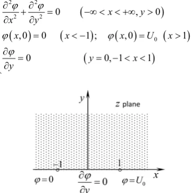
Figure 1 shows a cross section of a charged plane, in which the electric potential equal to zero within x< −1 on coordinate axis x, and the normal derivative of electric potential equal to zero within − < <1 x 1 on coordinate axis x, also the electric potential equal to U0 within x>1 on coordinate axis x. Now let us
solve aforementioned electric potential distribution above the charged plate. This boundary value problem can be written as
(
)
( )
(
)
( )
(
)
(
)
2 2
2 2
0
0 , 0
,0 0 1 ; ,0 1
0 0, 1 1
x y
x y
x x x U x
y x
y
ϕ ϕ
ϕ ϕ
ϕ
∂ ∂
+ = −∞ < < +∞ >
∂ ∂
= < − = >
∂
= = − < <
∂
(1)
DOI: 10.4236/jamp.2019.73039 538 Journal of Applied Mathematics and Physics This is the third kind boundary value problem of the Laplace’s equation, and there are two different boundary conditions on one of its boundary (y=0). It is difficult to solve the electric potential distribution directly. In order to solve this boundary value problem easily, first of all, the following transformation function
[5] is used
( )
arcsin z
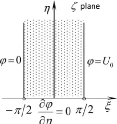
ζ = (2) Thus, the upper half plane of z plane is mapped onto a semi-infinite strip do-main of ζ plan by using above transformation function, and the boundary condition of the bottom of the semi-infinite strip domain is change into the second kind of boundary condition, that is 0
y ϕ ∂
=
∂ , as shown in Figure 2.
After the mapping function (2), the Equation (1) becomes
(
)
(
)
2 2
2 2
0
π 2 π 2
0 1 1, 0
0;
0 1 1, 0
U
ξ ξ
ϕ ϕ ξ η
ξ η
ϕ ϕ
ϕ ξ η
η
=− =
∂ +∂ = − < < >
∂ ∂
= =
∂
= − < < =
∂
(3)
Because ∂ϕη =0
∂ on the of the bottom of the semi infinite strip domain, and
other two sides of the semi infinite strip domain are parallel, so the electric field inside this domain is a uniform field, then the electric potential function of Equ-ation (3) is obviously
0 0
2 π
U U
ϕ
= +ξ
(4)Now let us express ξ using x and y. Because of the inverse function of the Equation (2) is z=sin
( )
ζ , therefore( )
( )
( )
( )
sin cosh , cos sinh
[image:3.595.314.434.560.687.2]x= ξ η y= ξ η (5) when 0< <ξ π 2, sin
( )
ξ or cos( )
ξ are not equal to zero, then we get the following formula form the formula (5)DOI: 10.4236/jamp.2019.73039 539 Journal of Applied Mathematics and Physics
( )
( )
2 2
2 2 1
sin cos
x y
ξ − ξ = (6)
For each changeless ξ, the focus of the hyperbola (6) is
( )
( )
2 2
sin cos 1
z= ± ξ + ξ = ± (7)
The horizontal axis length of the hyperbola (6) is 2sinξ , the absolute value
of the difference in distance of the from the point
( )
x y, to the two focal points of the hyperbola on the first quadrant is(
x+1)
2+y2−(
x−1)
2+y2 =2sin( )
ξ (8) By substituting Equation (8) into Equation (4), the electric potential distribu-tion funcdistribu-tion in the semi-infinite domain above the charged plane is expressed as(
)
2 2(
)
2 20 0arcsin 1 1
2 π 2
x y x y
U U
ϕ= + + + − − +
(9)
In order to give an intuitive image of the distribution of the electric field in the semi-infinite domain above the charged plane, and to verify the correctness of the conclusion of the results of the above research, next, the electric field line and the equipotential line diagram of the electric field in the semi infinite region above the charged plane are plotted by the mathematical software MATLAB, as shown in Figure 3. It can be seen that the electric field lines are perpendicular to the surface of the conductor and the equipotential lines and neither electric field lines emit from the boundary of the second kind of boundary condition (i.e.
0
y ϕ
∂ =
∂ ) nor electric field lines terminate on it. All of the above are the expected
[image:4.595.270.477.513.689.2]results, this shows that the research method in this paper is correct and its con-clusion is reliable.
Figure 3. The electric field lines and equipotential lines of the electric fields in a semi infinite domain above a charged plane.
x/m y/m
-5 0 5
0 1 2 3 4 5 6 7 8 9 10
0 10 20 30 40 50 60 70 80 90 100
equipotential line
DOI: 10.4236/jamp.2019.73039 540 Journal of Applied Mathematics and Physics
3. The Electric Field of a Charged Right Angle Domain
Figure 4 shows a cross section with an infinite long charged right angle domain, in which the electric potential equal to zero within y=0 on coordinate axis x, the electric potential equal to U0 within − < <1 y 1 on coordinate axis y, and
the normal derivative of electric potential equal to zero within y>1 on coor-dinate axis y. Now let us solve aforementioned electric potential distribution in a charged right angle domain. This boundary value problem can be written as
(
)
( )
(
)
( )
(
)
(
)
2 2 2 2 00 0, 0
,0 0 0 ; 0, 0 1
0 0, 1
x y
x y
x x y U y
x y x ϕ ϕ ϕ ϕ ϕ ∂ ∂
+ = > >
∂ ∂
= > = < <
∂
= = >
∂
(10)
This boundary value problem is the third kind boundary value problem of Laplace’s equation, and there are two different boundary conditions on one of its boundary (i.e. x=0). It is difficult to solve the electric potential distribution directly. In order to solve this boundary value problem conveniently, first of all, the following transformation function [6] is used
w u iv i z= + = (11)
By transformation (11), the domain on the z plane, shape like the quadrant, as shown in Figure 4, is mapped to the quadrant domain on the w plane, as shown in Figure 5, then Equation (10) becomes
(
)
( )
(
)
( )
(
)
(
)
2 2 2 2 00 0, 0
0, 0 0 ; ,0 1
0 0,0 1
u v
u v
v v u U u
v u
v
ϕ ϕ
ϕ ϕ
ϕ
∂ +∂ = > >
∂ ∂
= > = < < +∞
∂
= = < <
∂
(12)
Reusing the conformal transformation function as follows
( )
arcsin w
ζ = (13)
Thus, the domain on the w plane, shape like the quadrant, is mapped to a semi infinite strip domain on the ζ plane, and after the mapping, the boun-dary conditions at the bottom of the semi infinite strip domain be changed into the second kinds of boundary conditions, that is ϕ 0
η
∂ =
∂ , as shown in Figure 6.
By transformation (13), Equation (12) becomes
2 2
2 2
0
0 π 2
π 0 0,0 2 0; π 0 0,0 2 U ξ ξ
ϕ ϕ η ξ
ξ η
ϕ ϕ
ϕ η ξ
η
= =
∂ +∂ = > < <
∂ ∂ = = ∂
= = < <
∂
DOI: 10.4236/jamp.2019.73039 541 Journal of Applied Mathematics and Physics
Figure 4. The cross sectionof a charged right angle domain and its boundary condition.
Figure 5. The solvingdomain mapped and its boundary condition.
Figure 6. The solving domain remapped and its boundary condition.
Because ∂ϕη =0
∂ on the bottom of the semi infinite strip domain, and the
other two sides of the semi infinite domain are parallel, so the electric field in-side this domain is a uniform field, therefore, the electric potential function of the Equation (14) is obviously
0
2 π
U
[image:6.595.306.440.244.385.2] [image:6.595.303.442.432.571.2]DOI: 10.4236/jamp.2019.73039 542 Journal of Applied Mathematics and Physics Now let us express ξ by using x and y. Because of the inverse function of the Equation (13) is z=sin
( )
ζ , by using the same way of calculation as from for-mula (5) to (8), we obtain(
u+1)
2+v2 −(
u−1)
2+v2 =2sin( )
ξ (16) and by using formula (11), we get2 2; 2 2
y x
u v
x y x y
= =
+ + (17)
By substituting Equations (16) and (17) into Equation (4), hence the electric field distribution of the infinite long charged right angle domain is expressed as
2 2 2 2
0
2 2
2 1 2 1
2 arcsin
π 2
x y y x y y
U
x y
ϕ
= + + + − + − + +
(18)
In order to give an intuitive image of the electric field distribution in the charged right angle domain, and to verify the correctness of the conclusion of the above research, the electric field line and the equipotential line diagram of the electric field in the infinite long charged right angle domain are plotted by the mathematical software MATLAB, as shown in Figure 7. It can be seen that the electric field line is perpendicular to the surface of the conductor and the equipotential lines and neither electric field lines emit from the boundary of the second kind of boundary condition (i.e. 0
y ϕ ∂
=
∂ ) nor electric field lines
termi-nate on it, as shown in Figure 7. All of the above are the expected results, this shows that the research method in this paper is correct and the conclusion is re-liable.
4. The Electric Field in a Strip Region of Charged Condition
and Insulated Condition
Figure 8 shows the boundary condition of an infinite long strip domain. Now let us solve the electric potential distribution in an infinite long strip domain. This boundary value problem can be written as
(
)
( )
(
)
(
)
(
)
(
) (
)
2 2
2 2
0 0
0 ,0 1
0, 0, 1 ; , 0, 0
0 0 , 0 ; 0 , 1
x y
x y
y U x y y U x y
x y x y
y
ϕ ϕ
ϕ ϕ π
ϕ
∂ ∂
+ = −∞ < < +∞ ≤ ≤
∂ ∂
= − −∞ < < = = −∞ < < =
∂
= < < +∞ = < < +∞ =
∂
(19)
This boundary value problem is the third kind boundary value problem of Laplace’s equation, and there are two different boundary conditions on the boundary. It is difficult to solve the potential distribution directly. In order to solve this boundary value problem conveniently, the following transformation function [7] is used
(
π)
arcsin e z
DOI: 10.4236/jamp.2019.73039 543 Journal of Applied Mathematics and Physics Thus, the infinite long strip domain on the z plane is mapped to a semi-infinite long strip domain on the ζ plane, and the boundary condition at the bottom of the semi-infinite strip domain mapped are second kind of boundary conditions (i.e. ϕ 0
η
∂ =
∂ ), as shown in Figure 9. By using transformation
[image:8.595.263.487.173.360.2]func-tion (20), Equafunc-tion (19) becomes
[image:8.595.272.472.409.519.2]Figure 7. The electric field line and the equipotential line diagram in the infinite long charged right angle domain.
Figure 8. The charged strip domain and its boundary condition.
[image:8.595.298.451.559.700.2]DOI: 10.4236/jamp.2019.73039 544 Journal of Applied Mathematics and Physics
(
)
(
)
2 2 2 2 0 0 0 π0 0,0 π
;
0 0,0 π
U U
ξ ξ
ϕ ϕ η ξ
ξ η
ϕ ϕ
ϕ η ξ
η
= =
∂ ∂
+ = > < <
∂ ∂
= = −
∂
= = < <
∂
(21)
Because ϕ 0 η ∂
=
∂ on the bottom of the semi-infinite strip domain, and the
other two sides of the semi-infinite domain are parallel, so the electric field in-side this domain is a uniform field, therefore, the electric potential function of the Equation (21) is obviously
0
2 π
U
ϕ
= −ξ
(22)Form Equation (20), we obtain [8]
(
)
(
)
(
(
)
)
( )
(
)
(
(
)
)
( )
π 2π
2π
4π 2π π
4
2π 2π
4π 2π π
4
2π
ln e e 1
e sin 2π
1
e 2e cos 2π 1 sin arctan e sin π
2 e cos 2π 1
1 arctan
2 1 e sin 2π
e 2e cos 2π 1 cos arctan e cos π
2 e cos 2π 1
z z
x
x x x
x
x
x x x
x i y y y y y y y y
ζ − −
− − − − − − − − − − = − + + + + ⋅ − + = − + + ⋅ + +
(
)
(
)
(
(
)
)
2π 4π 2π
2π
π 4 4π 2π
2π
ln e e 2e cos 2π 1
2
e sin 2π
2e e 2e cos 2π 1 cos π
e cos 2π 1
x x x
x
x x x
x i y y y y y − − − − − − − − + + + + − − + + ⋅ + + (23)
By substituting the real part of the Equation (23) into Equation (22), hence the electric field distribution of the infinite long strip domain is expressed as
( )
(
)
(
(
)
)
( )
(
)
(
(
)
)
( )
2π
4π 2π π
4
2π 0
2π
4π 2π π
4
2π
e sin 2π
1
e 2e cos 2π 1 sin arctan e sin π
2 e cos 2π 1
, arctan
π 1 e sin 2π
e 2 cos 2π 1 cos arctan e cos π
2 e cos 2π 1
x
x x x
x
x
x x x
x y y y y U x y y
e y y
y ϕ − − − − − − − − − − + + ⋅ − + = + + ⋅ + + (24)
In order to give an intuitive image of the electric field distribution in the finite long charged strip domain, and to verify the correctness of the conclusion of the above research, the electric field line and the equipotential line diagram of the electric field in the infinite long charged strip domain are plotted by the mathe-matical software MATLAB, as shown in Figure 10. It can be seen that the elec-tric field lines are perpendicular to the surface of the conductor and the equipo-tential lines and neither electric field lines emit from the boundary of the second kind of boundary condition (i.e. 0
y ϕ ∂
=
∂ ) nor electric field lines terminate on it
DOI: 10.4236/jamp.2019.73039 545 Journal of Applied Mathematics and Physics
Figure 10. The electric field line and the equipotential line diagram in the electric field in a strip domain of the charged condition and insulated condition.
5. Concluding Remarks
The research method of computer numerical simulation has become the third research means other than the experimental research and the theoretical analysis. In this paper, by combining theoretical analysis with computer numerical simu-lation, the third boundary value problem of the Laplace’s equation is solved by using the conformal mapping method, and the visual image of the electric field distribution is given; the conclusion of this paper provides a new way of thinking and method for solving the complex electrostatic field boundary value problem and realizing the visualization of that. It is a new way of solving the complex electrostatic field boundary value problem, and it has a reference value for rele-vant scientific research and teaching.
Conflicts of Interest
The author declares no conflicts of interest regarding the publication of this pa-per.
References
[1] Xie, C.-F. and Yao, K.-J. (2006) Electromagnetic Field and Electromagnetic Wave. Higher Education Press, Beijing, 148-153.
[2] Xia, B.-L. (2004) On the Equivalent Feature of Laplance Equation with Third Boundary Value Problem and the Problem in the Variation Calculus. College Ma-thematics, 20, 365-368.
[3] Silalahi, F.T.R., Budhi, W.S., Adytia, D. and van Groesen, E. (2015) Numerical Solu-tion for Laplace EquaSolu-tion with Mixed Boundary CondiSolu-tion for Ship Problem in the Sea. AIP Conference Proceedings, 1677, Article ID: 030006.
[4] Simonov, N.A. (2017) Walk-on-Spheres Algorithm for Solving Third Boundary Value Problem. Applied Mathematics Letters, 64, 156-161.
https://doi.org/10.1016/j.aml.2016.09.008
[5] Saff, E.B. and Snider, A.D. (2007) Fundamentals of Complex Analysis with Applica-tions to Engineering and Science. 3rd Edition, China Machine Press, Beijing, 414-415.
Educa-DOI: 10.4236/jamp.2019.73039 546 Journal of Applied Mathematics and Physics tion Press, Beijing, 351-356.
[7] Saff, E.B. and Snider, A.D. (2007) Fundamentals of Complex Analysis with Applica-tions to Engineering and Science. 3rd Edition, China Machine Press, Beijing, 441, 584.