Disorder Effect on the Transmission of Second Harmonic Waves in One Dimensional Periodically Poled LiTaO3

(1)

http://www.scirp.org/journal/jmp ISSN Online: 2153-120X ISSN Print: 2153-1196

DOI: 10.4236/jmp.2019.104028 Mar. 19, 2019 432 Journal of Modern Physics

Disorder Effect on the Transmission of Second

Harmonic Waves in One-Dimensional

Periodically Poled LiTaO

3 Bahrami Omid

*

, Baharvand Abdolrahim, Bahari Ali

Department of Physics, Faculty of Science, Lorestan University, Khorram-Abad, Iran

Abstract

One of the methods for calculating electromagnetic wave dispersion in mul-ti-layer structures is the transfer matrix method. In this paper, we use the transfer matrix method for second harmonic generation in a nonlinear mul-tilayer structure. The nonlinear photonic crystals investigated in this paper are as one-dimensional multi-layered structures including ferroelectric mate-rials such as LiTaO3. Our goal is to investigate the effect of the disorder on the

transmission spectrum of electromagnetic waves. Our results showed that po-sitional disorder has different effects on the transmitting band and the gap band. The disorder in the transmitting band reduces the transmission coeffi-cient of the waves and increases the transmission coefficoeffi-cient of the waves in the gap band. Such work has not yet been done on nonlinear photonic crys-tals producing the second harmonic.

Keywords

Transfer Matrix Method, Nonlinear Photonic Crystal, Random Binary Medium, Transmission Spectra, Disorder Effect, Second Harmonic Waves

1. Introduction

In recent decades, the study of the transmission of waves in random systems has been highly studied because it plays an important role in understanding the opt-ical, mechanopt-ical, magnetic, and electrical properties of materials. The most im-portant theory in this case is Anderson’s theory. This theory is about electrons crossing in random systems [1] [2]. Although Anderson’s theory was initially about the transmission of electron waves in disordered systems, it was later ex-tended to other waves such as electromagnetic and acoustic waves.

How to cite this paper: Omid, B., Abdo-lrahim, B. and Ali, B. (2019) Disorder Ef-fect on the Transmission of Second Har-monic Waves in One-Dimensional Period-ically Poled LiTaO3. Journal of Modern Physics, 10, 432-442.

https://doi.org/10.4236/jmp.2019.104028

Received: February 19, 2019 Accepted: March 16, 2019 Published: March 19, 2019

(2)

DOI: 10.4236/jmp.2019.104028 433 Journal of Modern Physics

A weak disorder in 3D devices does not turn all of the extended modes into localized modes. That is; there is a series of transmission modes in the system. For strong disorder, due to the incoherent interference of waves, transmitted modes are exponentially localized. For one-dimensional systems, Anderson’s theory shows that all the passing modes are exponentially localized for any de-gree of disorder [2][3].

There are several models for one dimensional multi-layer system in which exponential localization is violated. For example a one-dimensional system with the periodic period consisting of two parts is known as a random-dimer model

[4][5]. In this type of system, there are modes that disorder does not affect them. Another model that violates Anderson’s localization in disordered one-dimensional systems is a long-range correlation model [6][7]. The tight-binding 1D model also violates the exponential localization in one-dimensional systems that occur for any disorder [8] [9]. Finally, the last model that produces non-localized states, unlike the one-dimensional Anderson model prediction, is called the “necklace” model [10]. This model has been used in a multilayer dielectric structure [11].

A periodic structure with a transmission spectrum that does not have any propagating modes in certain frequency regions is called the photonic crystal

[12]. Frequency spectrum, in which there are no propagating modes, is known as photonic band gap. Due to the vectorial nature of the electromagnetic waves, compared with the scalar nature of electron waves, the emission of electromag-netic waves in photonic crystals depends on its polarization and the wave prop-agation angle [13].

In a binary multi-layer structure made up of dielectric slabs, in which the opt-ical lengths of the layers are equal, putting the disorder in the order of the layers leads to the appearance of necklace modes in the photonic band gap [14]. By placing a positional disorder in a multilayer structure, when the optical length of layer is equal to a quarter wavelength, a series of transmission modes through the photonic band gap are created [15].

Photonic crystals contain ferroelectric materials, due to the unique properties that compensate for the phase mismatch in the second harmonic generation, which have been much considered. Second harmonic generation is investigated in multilayer nonlinear structures including ferroelectrics such as LiNbO3,

KTi-OPO4 and strontium barium niobate [16][17].

But until now, the effect of the disorder on the second harmonic generation (SHG) in the photonic crystals including ferroelectric materials has not been studied. We investigate the effects of positional disorder on the transmission spectrum of one-dimensional structures composed of lithium tantalite (LiTaO3).

(3)

in the nonlinear structure, a second harmonic wave is also produced.

This paper is organized as follows in Section 2 we focus on the details of the model and we derive the related transfer matrix. We also explain how we calcu-late the Transmission coefficient. In Section 3 we present and discuss our nu-merical results. Finally, Section 4 ends the paper with a summary of our results.

2. Model and Method

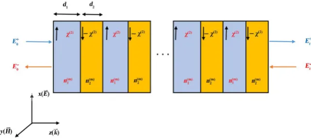
In this section, we study a multi-layered nonlinear structure, which changes the nonlinear parameter sign periodically in layers. In this structure, the scales of li-near and nonlili-near parameters are the same. The nonlili-near structure is divided into N periods of thickness d, and each period is divided into two homogeneous sections, Figure 1. Thickness and linear parameter (refractive index) and nonli-near parameter (second order susceptibility) for Section 1 are, respectively, dI,

( )r I

n and

χ

( )2 , while those for Section 2 are, d_II, n( )IIr and ( )2

χ

− _{, while}

,

r= f s is use for the fundamental field and second harmonic field, respectively.

Due to the fact that the refractive index of regions I ( ( )r I

n ) and II (n( )IIr ) are not

equal, its reflection will occur at each layer interface, resulting in between the transmitted and reflective waves in each layer, the phenomenon of interference will appear.

It is assumed that an electromagnetic wave with frequency ω incident from the left-hand side of the system and propagates in the direction of the z axis, so that the polarization of the electric field is in the x-axis direction. Our numerical calculations are based on the nonlinear transfer matrix method (TMM) [18][19]. In this method, the SHG process is divided into three stages: 1) First, the funda-mental field (FF), with the propagation in the structure, causes the macroscopic polarization of matter. 2) Since the material is non-linear, then the second-order nonlinear polarization is created in matter. And this nonlinear polarization ra-diates the second harmonic (SH) field in the structure. 3) This second harmonic field is propagated in the device, and it comes out in the form of a second har-monic signal.

In the first stage of the second harmonic generation, the fundamental and second harmonic fields follow the following equations:

(

)

( )

(

)

2

2 2

2 2 2 0

2

2 0 2

2

2 _NL

NL c

c

ω ω

ε

ω

µ

ω

ε ω

_{µ ω}

∇× ∇× − =

E E P

(1)

In which, εω, ε2ω, NL

ω

P , and 2

NL

ω

P are permittivity and nonlinear

polariza-tion at FF and SH frequencies. Because the nonlinear process is weak. As a result, the nonlinear process has no significant effect on the intensity of the fundamen-tal pump field (Given that the material we have used in this paper is ferroelectric (LiTaO3), whose second-order non-linear coefficient

χ

( )2 is 13.8 pm/V.

(4)

[image:4.595.214.535.76.218.2]

Figure 1. Multi-layered nonlinear structure. In each layer, the vectors represent the non-linear polarization direction.

obtaining the transmission coefficient. That is, the second-order nonlinear coeffi-cient is small, so the nonlinear process does not have a significant effect on the ini-tial wave intensity). So here we are using the non-depleted pump wave approxima-tion, E2ω Eω. Therefore, the above equations for the m-th layer are as follows

( )

2 ₂ 2 2 ₂ 2 2 0 2 d 0 d d 2 d f f m m s s

m m NL

k E z

z

k E z z ω µ ω   + =       + = −  

  P

(2)

where ( ) ( ) ( )0

f f f

m m

k =n k , ( ) ( ) ( )0

s s s

m m

k =n k , 0( )

f

k =

ω

c, and 0( ) 2

s

k =

ω

c. and also,

( )f m

n and n_m( )s show the refractive index of the pump waves and the second

harmonic, respectively in the mth slab; c,the speed of light is in vacuum

The first equation of coupling Equations (2) gives the fundamental electric field in the mth layer.

( )

(

( )( 1)

)

(

( )( 1)

)

e e

f f

m m m m

i k z z t i k z z t

f f f

m m m

E =E + − − −ω +E − − − − −ω (3)

where z0 is zero, zm =zm−1+dm and dm is the thickness of the mth layer.

( )f m

E + is the magnitude of forward plane wave and Em( )f

−

is the magnitude of backward plane wave at the left interface of the mth layer.

According to the continuity conditions on the boundary of the layers, we have the following matrix relation between the electric and magnetic fields passing through odd layer to even layer:

( )

( ) ( ) ( ) ( )

1 1 1 1

2 1 2 2

12

1 1 1 1 1

2 1 2 2

1 2

f f f

I II I II

m m i

f f f

m I I II I II m i

n n n n

E E E

T

E n n n n n E E

+ + + − − − − −     + −       = =   _ _    − +

  _ _    (4)

Using the matrix of dynamics and the matrix of propagation that are as follows.

( ) ( )

1 1

m f f

(5)

The general transfer matrix for the multi-layer structure is as follows

(

)

1 1 1

0 0

N II II II I I I

T =D− D P D D P D− − D (5)

This transfer matrix connects the fields at the beginning and the end of the structure, as follows

0 0 f f t f f t E E T E E + + − −     =    

    (6)

For harmonic fields that is produced in the structure, we use Equation (2) with 2

( )

( )2 ( )

( )

2

(

)

0

, f exp 2

NL m m

P ω z t =ε χ _E z _ −i ωt that yields to:

( ) ( ) ( ) ( )

(

)

(

)

(

)

(

)

(

)

( )

(

)

2 2 1 1 1 1

0 0 0 ₂

1 ₂ ₁

1 2 1 2 1

0 2 2 1 0 ₂ 2

1 2 2

0 0 0 f s s m m m

II I I I I

s s _f

m m _m

f f

I m m

II

m II II II II II

m

f f II m m II

E

E E

G SG G N B F SB A

E E _E

C E E

G N S

G B F N B A

C E E

G I N

+ + + − − − − − − ₋ − ₋ + − − − − + − − + − −       _ _  =  + − _ _     _ _     _ _   + −    

 _Ω 

 

+ − _ _

 Ω 

    + − _ _   (7) In which: ( ) ( ) ( ) ( ) ( )

2 2 2 2

0 0

2 2 2

4 4

, 4

l l

l s f l s

l l l

A C

k k k

µε χ ω µε χ ω

− − = = − ( ) ( ) ( ) ( ) ( ) ( ) ( ) ( ) 0 0 0 0 1 1 1 1

, 2 f f 2 f f

l s s l l l

l l s s

G B k n k n

n n k k       =_ ₋ _ = ₋        ( )

(

)

( )

(

)

exp 0 0 exp s l i i s l l ik d Q ik d     = _ ₋ _   ( )

(

)

( )

(

)

exp 2 0

,

0 exp 2

f l l l

f l l

i k d

F l I II

i k d

 

 

=_ _ =

 − 

 

1 1_, 1

II II II I I I II II II II

S=G Q G G Q G− − N =G Q G−

(6)

comparison with laboratory work). Using the intensity of waves, we have the following definitions for the nonlinear reflectance and nonlinear transmittance:

(

)

(

)

2

r

NL harm

pump

t

NL harm

pump I R

I

I T

I

=

(8)

where t r,

harm

I and Ipump are the intensities of the reflected or transmitted

har-monic and pump fields, respectively.

In our structure, it is assumed that the nonlinear photonic crystal are com-posed of periodically poled lithium tantalite (LiTaO3) crystal, whose nonlinear

susceptibility is ( )2

13.8 pm V

χ

= and The refractive index for lithium tantalite (LiTaO3) is given by the following dispersion formula [20]:

(

)

( )

2 2

2 2 2

2

, B b T E

n T A D

F C c T

λ λ

+

= + + +

−

−_ + _ (9)

where A=4.5284, B=7.2449 10× −3, C=0.2453, D= −2.3670 10× −2,

2

7.7690 10

E= × − , F =0.1838, b T

( )

=2.6794 10× −8

(

T+273.15

)

2,

( )

8

(

)

2

1.6234 10 273.15

c T = × − T+ .

Periodic polar ferroelectric (LiTaO3) crystals are described by modulations of

the nonlinear susceptibilities. An optoelectronic effect is used to produce the photonic band gap structure. This effect is the origin of the modulation of the refractive index of the layers in the photonic crystal. If the electric field E is ap-plied in the direction of the optical axis of the material, correction of refractive index and new refractive index (in odd layers) are as follows:

3

1 1 33

1 2

n = + ∆ = −n n n n r E (10)

where r33 is the optoelectronic coefficient of the material and E is the electric

field amplitude. Similar to the nonlinear optical coefficient, the optoelectronic coefficient of the material in different layers has different signs. So in reverse (even) layers the optoelectronic coefficient changes sign and the refractive index in these layers is written as follows:

3

2 2 33

1 2

n = + ∆ = +n n n n r E (11)

3. Numerical Results

We investigate a random binary structure constructed of N lithium tantalite (LiTaO3) layers. The positional disorder in the structure means the probability

(7)

[image:7.595.210.536.74.202.2]

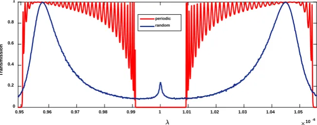
Figure 2. Transmission spectrum of periodic (red) and random (blue) binary structure with N = 70 layers. For the random system, to calculate the transmission coefficient quantity, averaging operations are performed on 3000 systems with different ordering. The placement of disorder has different effects on the transmitting and gap bands. The disorder results in the appearance of transmission modes in the middle of the gap band.

The transmission spectrum for periodic structures is a sequence of transmit-ting and stop bands. In the transmittransmit-ting band, there is a frequency in which the optical length of each layer is an integer multiple of half the wavelength in the vacuum. In other words, the phase change in each layer is equal to mπ, that m is the member of the integers. The nonlinear multi-layer structure for this incom-ing wave frequency is completely transparent. In the center of the stop bands, there are frequencies in which the optical length of each layer is odd multiples of one quarter wavelength. As a result, the phase change in these layers is equal to

(

m+12

)

π. For the random system, to calculate the Transmission coefficient

quantity, averaging operations are performed on 3000 systems with different ordering (Figure 2). The placement of disorder has different effects on the transmitting and gap bands. Firstly, the disorder does not affect the frequency in the transmitting band in which the optical length of each layer is an integer mul-tiple of half the wavelength. In other words, in a periodic and random structure at this frequency, the transmission coefficient is equal to the unit. Note that at this frequency, for each layer, the transfer matrix is a unit matrix (I). In this mode, independent of the existence and absence of disorder in the structure, is similar to the violation of Anderson localization in the random-dimer model. But, by placing disorder in the structure, the width of the transmission band is reduced. In the forbidden (gap) band, the disorder leads to the emergence of a series of transmitting modes. These mods are known as necklace modes.

In order to see the different effects of positional disorder in the transmitting band and the forbidden band, we plot the average transmission coefficient around the half- and quarter-wavelength modes as a function of the disorder in-tensity. In Figure 3 and Figure 4, q shows the disorder strength, in other words, q is equal to the probability that in the periodic structure (I, II, I, II, I, II, ∙∙∙, I, II), the ith layer, replaced with another layer. So q=0 is related to the periodic

structure and q=1 2 is a structure with complete disorder. The results are

shown in Figure 3 and Figure 4 for N = 70. In order to obtain the transmission 10-6

0.95 0.96 0.97 0.98 0.99 1 1.01 1.02 1.03 1.04 1.05

Transmission

0 0.2 0.4 0.6 0.8 1

(8)

[image:8.595.211.537.63.187.2]

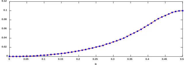
Figure 3. The average transmission coefficient as a function of the severity of the disorder, for the transmitting band. In this case, when the disorder increases, the transmission coefficient decreases, so Anderson’s localization is established. The averaging is per-formed on 3000 structures in different order and N = 70.

Figure 4. The average transmission coefficient as a function of the severity of the disorder, for the forbidden (gap) band. In quarter-wavelength modes, with increasing disorder, a series of transmitting modes are created, and thus a weak transmittance occurs at these frequencies. The averaging is performed on 3000 structures in different order and N = 70.

coefficient in random structures, the averaging is performed on 3000 structures in different order. Figure 3 for the transmitting band and Figure 4 for forbidden band.

[image:8.595.214.535.261.375.2]

For the average transmission coefficient around the half-wavelength reson-ance, when the disorder increases, the transmission coefficient decreases, so Anderson’s localization is established (Figure 3). Meanwhile, disorder effect in an around the quarter-wavelength resonance mode have a completely reverse result. As the disorder increases, the average transmittance increases (Figure 4). The reason for this is the appearance of transmitting modes in the forbidden band (Because in the periodic structure, in the gap band, the interference of the waves is non constructive. Using a disorder in the arrangement of the layers, the periodic structure that causes non-constructive interference of the waves and the transmission coefficient 0 in this frequency region (gaps) collapses. And with increasing disorder, the effect of the structure on the non-constructive interfe-rence of the waves decreases. As a result, the waves interact constructively. And there is a series of poorly transmitted modes in the gap band).

Figure 3 shows the average transmission coefficient in the transmitting band according to Anderson’s localization. In this case, the average transmittance coefficient decreases monotonically with increasing intensity disorder.

q

0 0.05 0.1 0.15 0.2 0.25 0.3 0.35 0.4 0.45 0.5

<T>

0.65 0.7 0.75 0.8 0.85 0.9 0.95

q

0 0.05 0.1 0.15 0.2 0.25 0.3 0.35 0.4 0.45 0.5

<T>

(9)

DOI: 10.4236/jmp.2019.104028 440 Journal of Modern Physics (a)

(b)

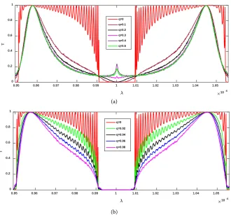
Figure 5. Transmission coefficient for different values of the disorder intensity. The number of layers is 70 and the averaging is performed on 2500 structures in different or-der. Figure 5(a) shows strong intensity disorder, in which case Anderson’s theory is vi-olated in the band gap. Figure 5(b) is for weak intensity disorders, in which case Ander-son’s localization is established.

[image:9.595.209.540.67.374.2]

While Figure 4 is a violation of Anderson’s theory, the disorder result in the emergence of a few resonance necklace modes that creates a small transmittance in gap band.

Figure 5 shows the transmission coefficient as a function of the collision wa-velength for different degrees of disorder. By increasing Severity of disorder, the bandwidth of transmission is reduced and a series of necklace mode is created in the gap bands which cause a slight increase in the transmission coefficient of electromagnetic waves. Figure 5(b) is for weak intensity disorders, in which case Anderson’s localization is established. Figure 5(a) shows strong intensity dis-order, in which case Anderson’s theory is violated in the band gap.

4. Results

We studied the transmittance spectra in a nonlinear structure composed of tan-talum lithium (LiTaO3). This system is a binary structure with N layer. The effect

of disorder on the transmitting and forbidden bands is quite distinct. For the transmission band, the disorder in the frequency at which the coefficient of transmission is equal to 1 does not affect. At this frequency, the transfer matrix of each layer is equal to the unit matrix (I). The lack of sensitivity of this fully

10-6 0.95 0.96 0.97 0.98 0.99 1 1.01 1.02 1.03 1.04 1.05

T

0 0.2 0.4 0.6 0.8 1

q=0 q=0.1 q=0.2 q=0.3 q=0.4 q=0.5

10-6 0.95 0.96 0.97 0.98 0.99 1 1.01 1.02 1.03 1.04 1.05

T

0 0.2 0.4 0.6 0.8 1

(10)

resonance mode is similar to the violation of Anderson’s theory in the ran-dom-dimer model. However, the width of the transmittance band in a disor-dered system is narrower than the width of the transmittance band of the peri-odic system. For the gap band, disorder lead to the appearance of several modes in the center of the band. These modes are called necklace modes, which are based on the hybridization of degenerate modes localized. The transmittance in the stop (gap) band increases with the disorder intensity. The transmittance in the transmitting band decreases with the disorder intensity.

Conflicts of Interest

The authors declare no conflicts of interest regarding the publication of this pa-per.

References

[1] Anderson, P.W. (1958) Physical Review,109, Article ID: 1492. https://doi.org/10.1103/PhysRev.109.1492

[2] Abrahams, E., Anderson, P.W., Licciardello, D.C. and Ramakrishnan, T.V. (1979)

Physical Review Letters, 42, Article ID: 673. https://doi.org/10.1103/PhysRevLett.42.673

[3] Kramer, B. and MacKinnon, A. (1993) Reports on Progress in Physics, 56, 1469. https://doi.org/10.1088/0034-4885/56/12/001

[4] Dunlap, D.H., Wu, H.-L. and Phillips, P.W. (1990) Physical Review Letters, 65, Ar-ticle ID: 88.https://doi.org/10.1103/PhysRevLett.65.88

[5] Phillips, P.W. and Wu, H.L. (1991) Science,252, 1805-1812. https://doi.org/10.1126/science.252.5014.1805

[6] de Moura, F.A.B.F. and Lyra, M.L. (1998) Physical Review Letters, 81, Article ID: 3735.

[7] Domínguez-Adame, F., Malyshev, V.A., de Moura, F.A.B.F. and Lyra, M.L. (2003)

[8] Theodorou, G. and Cohen, M. (1976) Physical Review B, 13, Article ID: 4597. https://doi.org/10.1103/PhysRevB.13.4597

[9] Fleishman, L. and Licciardello, D.C. (1977) Journal of Physics C, 10, L125. [10] Pendry, J.B. (1994) Advances in Physics, 43, 461-542.

https://doi.org/10.1080/00018739400101515

[11] Bertolotti, J., Gottardo, S., Wiersma, D.S., Ghulinyan, M. and Pavesi, L. (2005)

[12] Yablonovitch, E. (1987) Physical Review Letters, 58, Article ID: 2059. https://doi.org/10.1103/PhysRevLett.58.2059

[13] Fan, S.H., Villeneuve, P.R. and Joannopoulos, J.D. (1996) Physical Review B, 54, Article ID: 11245.https://doi.org/10.1103/PhysRevB.54.11245

[14] Sebbah, P., Hu, B., Klosner, J.M. and Genack, A.Z. (2006) Physical Review Letters, 96, Article ID: 183902.https://doi.org/10.1103/PhysRevLett.96.183902

(11)

DOI: 10.4236/jmp.2019.104028 442 Journal of Modern Physics [16] Piskarskas, A., Smilgevicius, V., Stabinis, A., Jarutis, V., Pasiskevicius, V., Wang, S.,

Tellefsen, J. and Laurell, F. (1999) Optics Letters, 24, 1053-1055. https://doi.org/10.1364/OL.24.001053

[17] Zhu, Y.Y., Fu, J.S., Xiao, R.F. and Wong, G.K. (1997) Applied Physics Letters, 70, 1793-1795.https://doi.org/10.1063/1.118694

[18] Bell, P.M., Pendry, J.B., Marin Moreno, L. and Ward, A.J. (1995) Computer Physics Communications, 85, 306-322.https://doi.org/10.1016/0010-4655(94)00131-K

[19] Lin, L.L., Li, Z.Y. and Ho, K.M. (2003) Journal of Applied Physics, 94, 811-821. https://doi.org/10.1063/1.1587011