Improved Dynamic K Coverage Algorithms in Mobile Sensor Networks

Imp

Abstract

In this pape the first alg covers an e buted mann second algo sented, com best experie not be the f (KVFPSO-L ledge and th gorithm, Im Simulation tion among

Keywords: W A

1. Introdu

Coverage is sensor netwo cified area is often used as WSNs [1]. In is usually req point in the erage levels ample, for th environment low value. On is always a m vironment su Even for the ments may v the coverage in dry season

proved

Rogh

1_Tec

2_Schoo

3_{School of}

Em Re

er, four PSO gorithm nam event in its s ner on its m orithm named mprised of V

ences of the final result a LA) is introd he feedback mproved KVF results show nodes, thus Wireless Sen Automata

ction

one of the mo orks, which is

monitored by s a measurem n surveillance quired to hav surveillance z for different he application

is friendly, th n the other han major concern uch as battlefie same applicat vary. For exam

level may be ns. Therefore, h

Dynam

hayeh Soleim

hnical and En l of Electrical Computer Eng mail:{soleima

eceived May 2

based distrib ed K-Covera ensing range mobile sensor d K-Coverag Virtual Force particles wer and cause ex

duced based from the act FPSO-LA is w that the pro maximizing

nsor Network

ost important concerned wit y sensors. Deg ment of the qu and monitori ve at least k se

zone (k-covera applications m n of home se he coverage lev

nd, having a h if sensors wo elds or chemic tion, the cover mple, for fore e low in rainy having a

user-mic K-C

Senso

manzadeh1, B

ngineering De l and Compute

gineering, Ira anzadeh.r, fara

26, 2010; revis

buted algorit age Particle e, implemen rs. The calcu ge Virtual Fo and KPSO re used to de tra movemen on which th tual impleme introduced, oposed proto network life

ks, K-Covera

issues in wire th how well a gree of coverag uality of servic

ing application ensors cover age) [2]. The may vary. For ecurity, where vel can be set high coverage l ork in a hostile cally polluted a rage level requ est fire detecti

seasons, but -defined param

Coverag

or Netw

ahani.ict}@gm

sed July 5, 20

thms are pre Swarm Opti ts Particle S ulation time orce directed algorithms. I etermine thei nts. Another he speed of p entation of th

in which sta ocols perform

e-time.

age, Event C

eless spe-ge is ce of ns, it each cov-r ex-e thex-e t to a

level e en-areas. quire- ions, high meter

k to requ

S ries cy i One slee such savi In -age WS dete loca dary netw T first dere

ge Algo

works

Farahani2, M

ad University g, Tehran Un of Science & T mail.com, mah

010; accepted A

esented to att imization (K warm Optim is considere d Particle Sw

In the first a ir speed. It is r algorithm n particles is co

he algorithm atic sensors a m well with r

Coverage, Par

represent the uirement in de Sensor nodes u as the source is the main ch e of the solut ep for extraneo h as S-MAC ing and sleep-n [2] a desleep-nse e in fields whe SN is consider ect events and ations to condu y conditions work in three d This article pre t algorithm, na ed as a big b

orithms

tain k-covera KPSO), each mization (PSO

ed as a big b warm Optimiz

and second p s possible th named KVFP

orrected by u m. To improv

are equipped respect to ba

rticle Swarm

coverage leve esigning a netw usually work w e of energy [4]

hallenge in se tions of powe ous nodes. He

[5] or T-MAC scheduling me sensor networ ere an event h red where stat d mobile senso

uct more adva to have k-cov different distri esents four PS amed KPSO th ottleneck, so

s in Mo

Fathy3 , Iran an, Iran Tehran, Iran ac.ir 010

age in the tar static senso O) algorithm bottleneck in zation (KVF proposed alg hat these resp PSO-Learnin using the exi ve performan d with learnin alanced energ

m Optimizatio

el is sometime work [3]. with small low

]; therefore, po ensor network er efficiency ence, use of M C [6] that sup echanisms is n rk is used to a has occurred. I

tic sensors are ors are dispat anced analysis verage in a m ibutions are pr SO based algo he calculation a second algo

obile

rget filed. In r which dis-m in a distri-n PSO, so a PSO) is pre-gorithms, the ponses might ng Automata isting know-nce of the al-ng automata. gy

consump-on, Learning

s a mandatory

w-power batte-ower efficien-k applications. is scheduling MAC protocols pports energy-necessary. attain K-cover In [7] a hybrid e deployed to tched to event . In [8], boun-mostly sleepy resented. orithms. In the

KVFPSO is presented comprised of Virtual Force and KP- SO algorithms and as the result, less energy is consumed.

The other algorithm named KVFPSO-LA is intro-duced, based on which the speed of particles is corrected by using the existing knowledge and the feedback from the actual implementation of the algorithm, in addition to using the law of virtual force. In this method, there will be less movement and re-location to achieve the desired result. Finally a new algorithm named Improved KVFPSO- LA is introduced, in which static sensors are equipped with learning automata. As the result, only the required numbers of mobile nodes are re-located.

2. System Model

In this paper, a mobile sensor network is a collection of the mobile nodes, which have mobility and are able to change their position based on networks dynamics or requirements. The system model is as followings:

 Mobile sensors are aware of their location by using locating algorithms [9].

 1-coverage is set up by using the method mentioned in [10] with minimum number of sensors and using the least amount of energy in the concerned field. All mobile sensors used for 1-coverage will be mentioned as static sensors.

 The communication range of sensors is greater or equal to their sensing range. As the result, static sensors are connected to each other. (Rc > = 2Rs)

 Covering detection model in these algorithms is Bi- nary Detection Model [11].

 Static sensors use to detect an event that has oc-curred in their sensing range and determine a coverage degree, based on the size of the event and environmental situations [3]. Then, based on the methods, which will be discussed later, they would increase coverage degree for that event to a determined extent.

 These protocols consist of five phases:

1-Initialization Phase, 2-Proxy Sensor Selection Phase,

3-Creating Mobile Sensor List Phase, 4-Creating

Par-ticle List Phase, 5-Running the Algorithm Phase

Phases 1-4 are in common within all proposed algo-rithms and only the last phase varies, which will be dis-cussed in herewith.

3. Algorithms Implementation Phases

3.1. Initialization Phase

In this phase, all mobile sensors would broadcast one hello message in the network. Static sensors in their commu-nication range, which have received this message which would in response, create and send a feedback message

consisting of two fields: identification number of static sensor and the location of the static sensor.

3.2. BProxy Sensor Selection Phase

In this phase, the mobile sensors should select one among many static sensors, which have sent feedback message to them. Therefore, a proxization probability is determined for each static sensor, which will be calculated using Equ- ation (1). Then, the mobile sensor will choose as its pro- xy the static sensor, which has the highest probability. If more than one sensor has equal probability, the proxy selection will be done based on order of receiving me- ssages, sending to it a delegate proxy request consisting of three fields. These would include the mobile iden- tification number, level of remaining energy and the lo-cation where in these fields are initialized in sequence with mobile sensor Mac address, mobile energy level and its location. From there on, all relocations of mobile sen- sors shall be done under their proxy sensors.

 

1 1 / m

i i

i

P a d d



 



d The distance between proxy (1)

i

node a and the mobile node

In this equation, m refers to the number of static sen-sors which have sent a feedback message for the mobile. The distance between the static sensor and the mobile is calculated by using the Euclidean distance.

After all mobile sensors have selected a proxy for themselves; they go to the sleep mode to cut down on energy consumption using the method mentioned in [5] and [6]. If an event occurs in their proxy’s sensing area or if selected as appropriate for relocating, as per a re-quest of other static sensors from its proxy, its proxy will wake it up by sending an awakening message to it.

3.3. Creating Mobile Sensor List Phase

This phase will be started by any static node, which de-tects an event in its sensing range. When the static sensor detects an intruder in its sensing range, it will determine how many mobile sensors are needed according to the size and bigness of the intruder and environmental situa-tions; meaning that in this phase it calculates the size of

K. For example, it can be said that K is a coefficient of the size of the intruder, for instance it needs five mobile sensors (6-coverage) for a panzer and two extraneous mobile sensors (3-coverage) for a soldier.

If the number of its mobile sensors is greater or equal to K, those of its sensors with less distance, compared to the sensing range with the event, are awakened with a message. The other sensors are put in a list named the list

of mobile sensors and advances to the next phase.

Otherwise, the following might occur:

If the number of mobile sensors is less than K, like the previous phase, those of its sensors which have less dis-tance than the sensing range to the event are awakened and the other sensors are put in the list of mobile sensors. It would then assess the degree of coverage, deduct it from K, and the final amount will determine the number of mobiles which should be taken from the neighbors. Subsequently, it would send a message of request to its neighboring static sensors, which would include ID num- ber of the static sensor (proxy) and location of the event. The adjacent static sensors which receive the message would evaluate it and might undertake either of the fol-lowing actions:

 If, there is no event in its sensing range and has no need for its mobile sensors, in a message to static sensor, the mobile requester would send the list of mobiles. This message would include its own ID number as well as that of its other mobiles and the location of its mobiles and the level of energy.

 If the neighboring sensor has also detected an event and its mobile sensors are engaged, then even if it has extraneous mobiles (i.e. the number of its mobiles are more than the number of K), it would give a negative reply to the requesting proxy. This is because there is the possibility that it again detects an event in the near future in its sensing range and might need its mobiles.

The requesting static sensor, given the amount of K, gives a positive response to those static sensors, which fulfill its need. Therefore, it takes the specifications of its mobile sensors and puts them in the list of mobile sen-sors. Thus, a list, including mobile sensors on which algorithm will be implemented, is created.

3.4. Creating Particle List Phase

Each static sensor, which has discovered an event in its sensing range, starts this phase after creating a list of mobile sensors, creating its particle list. In this section, a record will be attributed to each sensor existing in the mobile sensors’ list, which would include ID fields, loca-tion and energy level of the mobile sensor. At the same time, an initial speed is by coincidence attributed to it.

3.5. Running the Algorithm Phase

3.5.1. K-Coverage Particle Swarm Optimization (KPSO) Algorithm

This algorithm is implemented in distributed form by

static sensors, which have detected an event in their sen- sing range. In this algorithm, each static sensor, which de- tects an event in its sensing range, implements 1-4 phas-es and thus, creatphas-es its particle list. Then, it implements the PSO algorithm on its particles [11]. In this algorithm, the function fitness will be the distance between the mo-biles and the location of the event. Implementing this algorithm will continue until maximum number of repe-tition is achieved or the determined degree of coverage is attained by the proxy sensors for the event.

3.5.2. K-Coverage Virtual Force Directed Particle Swarm Optimization (KVFPSO) Algorithm

In KPSO algorithm, although the desired result is achi- eved, but the calculation time in this algorithm is a big bottleneck. Also, the speed of particles in this algorithm is determined only by using the local and global best experiences. This is while, there is the possibility that these might not be the best final results and cause extra and repeated movements.

To counter this problem, the law of virtual force has been used to determine the speed of particles in this al-gorithm. To do this, the locations of events are consi-dered regions with preferred coverage area and in a cir-cular shape. (Regions with preferred coverage area are regions where mobile sensors are attracted towards these regions by a force of attraction). The center of the circle is presumed as the location of the event and the radius of the circle is presumed as the sensing range of the sensors. Regions with preferred coverage are shown with Am and

the force of attraction applied to the sensor moving to-wards the location of the event is calculated as the fol-lowing [11]:





0

Apre Am iAm iAm Am

iAm

W P if r d r C

F

otherwise

    

  

 (2)

where r and c are the sensing range and communication range of mobile sensors. rAm and pAm are the radius and importance level parameter of the area of preferential coverage Am, wApreis a measure of the attractive forces exerted by obstacles , diAmis the distance between si and

Am,αiAm is the orientation of a line segment from sito Am. KVFPSO algorithm also is a distributed algorithm wh- ich is implemented by any static sensor which has detected an event in its sensing range. In this algorithm, the follow-ing equation is used to determine the speed of particles:

vij (t + 1) = w(t)* vij(t)

+ c1 * r1i(t) *(pbestij(t) – positionij(t))

+ c2 * r2i(t)* (gbestij(t) – positionij(t))

+ c3*r3i(t)*gij(t) (3) where vij(t) and positionij(t) represent the position and velocity of ith particle in the jth dimension at time t.

dimension and gbestij(t) is the global best position. r1i(t) and r2i(t) are two separate random function in the range [0,1]. c1, c2 are learning factors. The velocity of particle

in each dimension is limited to the Vmax[i] which i is the index of dimension. c3 is acceleration constant, r3i(t) is also a random function in the range [0,1] which is inde-pendent to r1i(t) and r2i(t), gij(t) is the prolepsis motion suggested by virtual force of ith particle in jth dimension [11] , which is computed by:

 

 

 1 ( , ₂₎

( , 2)

1 1

( , ₂₎ 1 ( , ₂₎

1 ( , 2)

( , 2)

( )

j i xy

j i xy

j i

F x

j i xy ij

j i

F y

j i xy

F

MaxStep e j odd F

g t

F

MaxStep e j even F



 





 

  

    

 _{  }

 

(4)

where the superscript of each parameter presents the in- dex of particles and the index of wireless sensor nodes which the virtual force exerts on, the subscript presents the coordinate of the virtual force. The correlative virtual forces are carried out by Equation (2).

In this algorithm, in addition to using the local best experience and the global best experience, the law of virtual force is also used to determine the speed of the particles. Adding this force to the speed of particles cau- ses them to move towards the location of the event at a faster pace. As the result, the algorithm achieves result with less number of repetitions and mobiles move more objectively. Therefore, in this method, there will be less re-location to achieve the desired result, causing less ener- gy consumption.

3.5.3. K-Coverage Virtual Force Directed Particle Swarm Optimization - Learning Automata (KVFPSO-LA) Algorithm

In the standard PSO algorithm, the responsibility to strike a balance between global and local search is with the me- dian coefficient. This coefficient determines how much of the particle’s current speed was used in determining its speed in the next phase. However, in [12], a new algo-rithm has been recommended which uses learning auto-mata to regulate the method of searching for particles. It is the learning automata which determine in each step that particles continue in their current route or follow the best particles found so far. Using the learning automata has two advantages: First, the existing knowledge can be used to determine the trend of changes in the medial weight, and second, the trend can be corrected in the ac- tual environment by using the feedback from implemen-tation of algorithm.

Here, a new algorithm is introduced by the name of KVFPSO-LA to achieve K degree of coverage in regions

where an event has occurred. This algorithm, like the other two algorithms are distributed algorithms which are im-plemented on static sensors which have detected an event in their sensing range. The implementation phase of this algorithm is such that after implementing the first 4 pha- ses and creating its particles list, the KVFPSO-LA algo-rithm is implemented as the following:

In this algorithm, it is assumed that the static sensors are equipped with learning automata. The used LA has two actions which are “Follow the best” and “Continue your way”. Until the desired goal is met or maximum number of iterations is done, the following steps should be repeated.

 LA selects one of its actions based on its probability vectors.

 Based on the selected action, the method of velocity updating for particles is selected and then the particles update their velocity and position.

 According to particles’ updating results, a reinforce- ment signal is generated which will be used to update the probability vectors of learning automaton.

The selected action of LA in any iteration specifies the velocity updating method of particles for that iteration. Selecting “Follow the best” action means that just follow- ing the best self experience and best team experience has effect on the velocity of the particle in the next iteration and the current particle’s velocity is ignored. In this case, the velocity update of the particles is done according to Equation (5). If the “Continue your way” action is select- ed, the new velocity of the particle will be equal to its current velocity.

vij (t + 1) = c1 * r1i(t) * (pbestij(t) – positionij(t))

+ c2 * r2i(t)* (gbestij(t) – positionij(t))

+ c3*r3i(t)*gij(t)

(5) As a matter of fact, the selection of “Follow the best” action causes a local search around the best particle and selection of “Continue your way” action has the effect of doing global search and discovering new unknown parts of the search space. The used LA is responsible for learn- ing probability distribution and balancing between local and global search. Evaluating the selected action is done by comparing each particle’s new position with its old position. If a specific percent of population (Cimp) are improved, the selected action will be evaluated as posi-tive and in the other cases it will be evaluated as a nega-tive action.

re-location for achieving the desired result and therefore, there will be less energy consumption compared to pre-vious algorithms.

3.5.4. Improved KVFPSO-LA Algorithm

In previous algorithms, the algorithm is implemented on all particles existing in the particles list, even if the number of these particles (mobile nodes) is more that the required amount of K. As a result, with implementation of this algorithm, more mobiles than required would mo- ve towards the location of the event and cause excessive use of energy.

To overcome this problem, it is assumed that each static sensor which detects an event in its sensing range is equipped with the learning automata and uses this learning automata to determine the particles (mobile nodes) on which the algorithm is implemented. It then moves towards the location of the event. The implemen-tation phases are as such that the static sensor, which detects an event in its sensing range, implements phases 1-4 and creates its particles list. The static sensor then, given its particles list, creates a learning automaton who- se number of actions is equal to the number of particles existing in the particles list. In fact, there is a one-to-one correspondence between the learning automata’s actions and the particles existing in the list. In this phase, the learning automata will attribute the probability of an ini-tial selection equal to 1/r (r is the number of particles in the list). Then, using the following equations, it will give reward or penalty for possible selection of its particles and thus, the most appropriate particles are selected for re-location towards the event. The implementation results show that by applying these equations, those mobiles, which have higher energy level and lesser distance from the event have the higher probability of being selected.

When the energy of the mobile we want to re-locate:  is less than 50 percent of the average energy of oth-er nodes, the selected node is penalized based on the 3β

parameter which is calculated using the following men-tioned parameter:

 









)]

i

i j

y AveEnergy Enregylevel a d a l y AveEnergy

dist between event and farthest node to event      

  (6)

 is more than 50 percent and less than 80 percent of the average energy of other nodes, the selected node is penalized according to the following parameter:

 

(1 )

30 i

P

Energylevel a AveEnergy

V 



  (7)

 is more than 80 percent and less than 100 percent of

the average energy of other nodes and the distance be-tween this node from the destination, among other nodes, is minimum. In such case the node is rewarded based on parameter α.

 

1 1[(

( , )) / (

)]

i

i j

y Enregylevel a

dist between event and farthest node to event d a l y AveEnergy

dist between event and farthest node to event      



  (8)

 is more than the average energy of other mobile nodes. In such case, the mobile node is awarded based on

α parameter.

λ1 and λ2 respectively determine the minimum amount

acceptable for the reward and penalty. Taking into ac-count the scale difference between distance and energy, the y parameter is regulated in way that these two terms are placed in an almost equal scale and ψ1 and ψ2 are

regulated in such a way that the amount of parameters α and β do not exceed a specific limit.

After the probability of selecting the mobile nodes is determined by using the above-mentioned equations, k

particles (mobile nodes) which have the highest selection probability are selected for covering the event and then one learning automata is allocated to each of the selected particles. Each learning automata is in fact the core of the particles, which guides its movement within the search space. Allocation of learning automata to each of the particles causes each particle to make decisions for de-termining the type of its movement without considering the movement of other particles and by using the result of its current movement in the environment. Each learn-ing automata has two actions of “follow the best” and “continue your way”. When an automata allocated to a particle chooses the action of “follow the best”, it means that the particle, according the Equation (5), moves to-wards the best location met by the group (gbest) and best location which has met so far (pbest) to move in the search space with the zero weight motion inertia. If the learning automata of each particle select the action of “continue your way”, it would mean that the particles is moving within the space at a current velocity and will continue the current way [13].

The algorithm in this method is as the following: 1) The phase of creating the particles list, for selected particles, is implemented.

2) The probability range of selection action of each particle’s learning automata is measured.

3) As long as the maximum number of steps are taken or the desired objective is achieved, phases 4 to 9 are repeated:

5) If the learning automata allocated to ith particle se-lects “follow the best”, the speed of the particles is up-dated according to Formula (5).

6) If the learning automata allocated to the particle se-lects “continue your way”, the speed of the particle will be equal to its previous speed.

7) Considering the selection action, the method of up-dating the speed of the particles is determined and then, particles will update their speed and location.

8) If the new location of the particle improves com-pared to its previous location, the particle will be award- ed for the action it selected. Otherwise, the action will be penalized.

9) The action selection probability range of the learn-ing automata is corrected.

Thus, the selected particles will move towards location of the event and achieve the required degree of coverage. Given that in this algorithm, only the required number of particles will be re-located and each particle will deter-mine the type of its action in the next phase according to the result of its implementation in the previous phase, thus less energy will be consumed.

4. Experimental Results

In this section, the performance of our algorithms will be evaluated by simulations. A 40 m × 40 m rectangle sen- sing field will be set up, in which there are several mo-bile sensors randomly deployed. Each momo-bile sensor has an initial energy reserved for movement and the moving energy cost per meter is set to 8.27 J.

A number of these mobile nodes were used for creat-ing 1-coverage and the rest are used for increascreat-ing cov-erage in case of the occurrence of an event. The sensing range of these sensors is equal to 5 m and their commu-nication range 20 m. It will be assumed that there are 5 events in specific locations in the space, and determined the results of implementation for these 5 events for dif-ferent coverage degrees. The parameters for virtual force are set as WApre = 1, Maxstep = 0.2 r = 1 m according to the discussion in [14]. The acceleration constants of PSO are set as c1 = c2 = c3 = 1 and λ1 and λ2 parameters are

measured equal to 0.1. The numbers of used particles in all PSO algorithms are 10.

For calculating the level of energy consumed by each mobile node by one unit, the following-mentioned equa-tion can be used, using the reference [7]:

( , ) move i j

W  d a l (9)

∆move is the energy required to move a sensor one-unit distance (∆move = 8.27), d(ai ,lj) is the Euclidean distance from ai’s current position and point lj is the point which mobile node will move there.

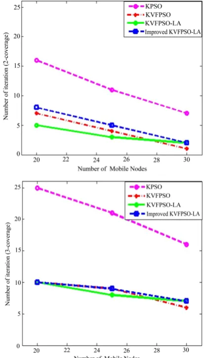
Figure 1 shows that for each one of the mentioned

al-gorithm, it will achieve the result with less number of repetitions with an increase in the number of mobile nodes. By comparing the number of repetitions in all four algorithms, it can be noted that the KPSO algorithm has the highest number of repetitions. This is because the speed of particles and their location are determined only through the previous phase on following up the local and global best experiences. Given that there is the possibili-ty of the local and global best experiences not achieving the final result, this cause the algorithm to achieve the result through higher number of repetitions. Comparing with KPSO algorithm, the KVFPSO algorithm has better performance and achieves the final result with less num-ber of repetitions. This is because, as it was mentioned, the law of virtual force has been used to determine the speed of particles and so more objective-oriented and more organized particles move towards the location of event. The KVFPSO-LA algorithm achieves the best result compared to the two previous algorithms because in ad-dition to using the law of virtual force, the speed of the particles is determined by taking into considering the

feedback from the actual implementation environment. In the improved KVFPSO-LA algorithm, since algo-rithms acts on less number of particles, the number of re- petitions is greater than or equal to KVFPSO and KVFPSO- LA algorithms.

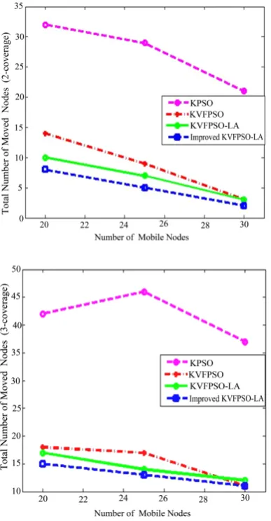
Figure 2 shows a comparison of the number of mobile

nodes that relocated to reach a certain degree of coverage. Number of these nodes will decrease when total number of mobile sensors increase; because the proxy node which detected the event in its sensing range has more mobile node to use and it has no need to make request to its neighbor proxy nodes. So the proxy node will send a message to the mobile nodes which have less distance with the event than the sensing range and wake up them to detect the event.

The KVFPSO algorithm, compared to KPSO, has less number of repetitions and as the result less number of re-located mobile nodes, due to the force of attraction that taken the mobiles towards the location of the event.

Figure 2. A comparison of the number of mobile nodes that relocated to reach a certain degree of coverage.

As it was mentioned before, the KVFPSO-LA algo-rithm, in comparison with the two previous algorithms, uses the result of the feedback from the movement of its particles in the actual environment, in addition to using the law of virtual force. Therefore, the result is achieving in less number of repetitions and less number of re-loca- ted nodes.

In the improved KVFPSO-LA algorithm, because it is implemented on the required number of particles, each particle determined the type of its movement in the next phase without considering of the movement of other par-ticles, and only taking into account the result achieve from its own implementation in the previous phase. Th- erefore, the number of re-locations is less and particles move more objectively.

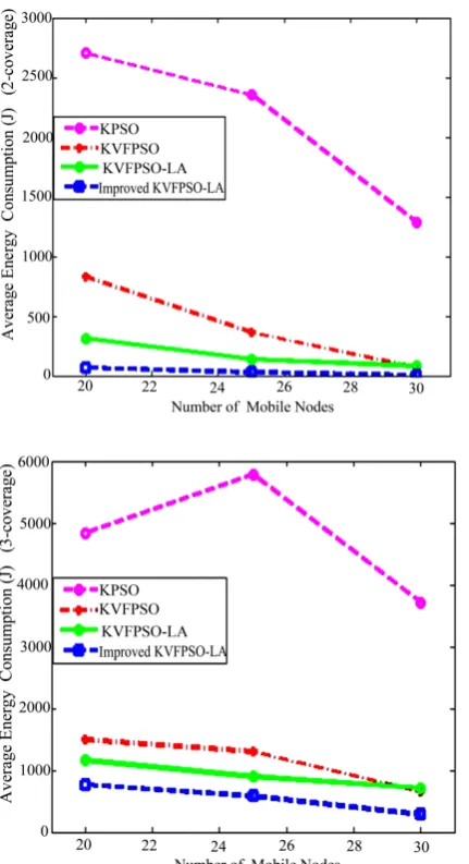
Figure 3 and Figure 4 show the Average Moving Dis-

tance and Average Energy Consumption for each relo-cated mobile sensor, respectively. As the figures demon-strate, for a specific level of coverage, by increasing num- ber of mobile nodes, Average Moving Distance and Aver-

Figure 4. Average energy consumption for each relocated sensor.

age Energy Consumption decrease.

In the improved KVFPSO-LA algorithm, because it is implemented on the required number of particles, each particle will determine the type of its movement in the next phase according to the result of its own implemen-tation in the previous phase. So, mobiles move within a shorter distance compared the other three algorithms.

By studying these four figures, it can be noted that by using the improved KVFPSO-LA and KVFPSO-LA al-gorithms, the mobiles have to travel within a shorter dis-tance compared to other two algorithms and therefore, they consume less energy.

5. Conclusions

In this paper four PSO based algorithms to achieve k-

coverage are proposed. In the KPSO, each static sensor which detects an event, implements PSO algorithm in a distributed manner on its mobile sensors. The calculation time is considered as a big bottleneck. So KVFPSO is proposed, comprised of Virtual Force and KPSO algo-rithms that resulted in less energy consumption. KVFPSO- LA is proposed based on which the speed of particles is corrected by using the existing knowledge and the feed-back from the actual implementation of the algorithm, in addition to using the law of virtual force. As the result, this algorithm achieves the final result with less number of repetitions. Finally, Improved KVFPSO-LA is pro-posed, in which static sensors are equipped with learning automata. By using these automata only the required numbers of mobile nodes are re-located. The experi-ments demonstrated the performance of the four algo-rithms and the Improved KVFPSO-LA was best in most cases.

6. References

[1] J. P. Sheu, G. Y. Chang and Y. T. Chen, “A Novel Ap-proach for K-Coverage Rate Evaluation and Re-Deploy- ment in Wireless Sensor Networks,” IEEE Global Tele-communications Conference, New Orleans, 2008, pp. 1-5. [2] A. Yahyavi, L. Roostapour, R. Aslanzadeh and N. Yazdani,

“DyKCo: Dynamic K-Coverage in Wireless Sensor Net-works,” IEEE International Conference on Systems, Man and Cybernetics, Singapore, 2008, pp. 2804-2809. [3] Y. S. Li and S. Gao, “Designing K-Coverage Schedules in

Wireless Sensor Networks,”Journal of Combinatorial Op- timization, Vol. 15, No. 2, 2008, pp. 127-146.

[4] F. Ye, G. Zhong, S. Lu and L. Zhang, “PEAS: A Robust Energy Conserving Protocol for Long-Lived Sensor Net- works,” Proceeding of the 10th IEEE International Con- ference on Network Protocols,Paris, 2002, pp. 200-201. [5] W. Ye, J. Heidemann and D. Estrin, “Medium Access

Control with Coordinated Adaptive Sleeping for Wireless Sensor Networks,” IEEE/ACM Transactions on Network- ing, Vol. 12, No. 3, 2004, pp. 493-506.

[6] T. V. Dam and K. Langendoen, “An Adaptive Energy- Efficient MAC Protocol for Wireless Sensor Networks,” Proceedings of the 1st International Conference on Em- bedded Networked Sensor Systems, Los Angeles, 2003, pp. 171-180.

[7] Y. C. Wang, W. C. Peng, M. H. Chang and Y. C. Tseng, “Exploring Load-Balance to Dispatch Mobile Sensors in Wireless Sensor Networks,” Proceedings of 16th Inter- national Conference on Computer Communications and Networks, Honolulu, 2007, pp. 669-674.

[8] S. Kumar, T. H. Lai and J. Balogh, “On K-Coverage in a Mostly Sleeping Sensor Network,” Wireless Networks, Vol. 14, No. 3, 2006, pp. 277-294.

Personal Communications, Vol. 7, No. 5, 2000, pp. 28-34. [10] J. Xiao, L. L. Sun and S. Zhang, “Distance Optimization

Based Coverage Control Algorithm in Mobile Sensor Network,” IEEE International Conference on Systems, Man and Cybernetics, Singapore, 2008,pp. 3321-3325. [11] X. Wang, S. Wang and J. J. Ma, “An Improved Co-Evolu-

tionary Particle Swarm Optimization for Wireless Sensor Networks with Dynamic Deployment,” Sensors, Vol. 7, No. 3, 2007, pp. 354-370.

[12] M. Sheybani and M. R. Meybodi, “PSO-LA: A New Mo- del for Optimization,” Proceedings of 12th Annual CSI

Computer Conference of Iran, Shahid Beheshti University, Iran, 2007, pp. 1162-1169.

[13] M. Hamidi and M. R. Meybodi, “New Learning Auto- mata Based Particle Swarm Optimization Algorithms,” Proceedings of the 2nd Iranian Data Mining Conference, Amirkabir University of Technology, Iran, 2008.