Efficient Sequence Learning with Group Recurrent Networks
Fei Gao1,2, Lijun Wu3, Li Zhao2, Tao Qin2, Xueqi Cheng1 and Tie-Yan Liu2 1Institute of Computing Technology, Chinese Academy of Sciences
2Microsoft Research
3School of Data and Computer Science, Sun Yat-sen University
{feiga,lizo,taoqin,tie-yan.liu}@microsoft.com;
[email protected]; [email protected]
Abstract
Recurrent neural networks have achieved state-of-the-art results in many artificial in-telligence tasks, such as language modeling, neural machine translation, speech recognition and so on. One of the key factors to these successes is big models. However, training such big models usually takes days or even weeks of time even if using tens of GPU cards. In this paper, we propose an efficient architecture to improve the efficiency of such RNN model training, which adopts the group strategy for recurrent layers, while exploiting the representation rearrangement strategy be-tween layers as well as time steps. To demon-strate the advantages of our models, we con-duct experiments on several datasets and tasks. The results show that our architecture achieves comparable or better accuracy comparing with baselines, with a much smaller number of pa-rameters and at a much lower computational cost.
1 Introduction
Recurrent Neural Networks (RNNs) have been widely used for sequence learning, and achieved state-of-the-art results in many artificial intelli-gence tasks in recent years, including language modeling (Zaremba et al., 2014; Merity et al.,
2017), neural machine translation (Sutskever et al., 2014; Bahdanau et al., 2014), and speech recognition (Graves et al.,2013).
To get better accuracy, recent state-of-the-art RNN models are designed toward big scale, in-clude going deep (stacking multiple recurrent lay-ers) (Pascanu et al.,2013a) and/or going wide (in-creasing dimensions of hidden states). For exam-ple, an RNN based commercial Neural Machine Translation (NMT) system would employ tens of layers in total, resulting in a large model with hun-dreds of millions of parameters (Wu et al.,2016). However, when the model size increases, the com-putational cost, as well as the memory needed for
the training, increases dramatically. The training cost of aforementioned NMT model reaches as high as 1019 FLOPs, and the training procedure spends several days with even 96 GPU cards (Wu et al.,2016) – such complexity is prohibitively ex-pensive.
While above models benefit from big neural networks, it is observed that such networks often have redundancy of parameters (Kim and Rush,
2016), motivating us to improve parameter ef-ficiency and design more compact architectures that are more efficient in training while keeping good performance. Recently, many efficient archi-tectures for convolution neural networks (CNNs) have been proposed to reduce training cost in com-puter vision domain. Among them, the group con-volution is one of the most widely used and suc-cessful attempts (Szegedy et al., 2015; Chollet,
2016;Zhang et al.,2017b), which splits the chan-nels into groups and conducts convolution sepa-rately for each group. It’s essentially a diagonal sparse operation to the convolutional layer, which reduces the number of parameters as well as the computation complexity linearly w.r.t. the group size. Empirical results for such group convolu-tion optimizaconvolu-tion show great speed up with small degradation on accuracy. In contrast, there are very limited attempts for designing better archi-tectures for RNNs.
Inspired by those works on CNNs, in this pa-per, we generalize the group idea to RNNs to con-duct recurrent learning in the group level. Differ-ent from CNNs, there are two kinds of parame-ter redundancy in RNNs: (1) the weight matrices transforming a low-level feature representation to a high-level one may contain redundancy, and (2) the recurrent weight matrices transferring the hid-den state of the current step to the hidhid-den state of the next step may also contain redundancy. There-fore, when designing efficient RNNs, we need to consider both the kinds of redundancy.
We present a simple architecture for efficient sequence learning which consists ofgroup recur-rentlayers andrepresentation rearrangement lay-ers. First, in a recurrent layer, we split both the input of the sequence and the hidden states into disjoint groups, and do recurrent learning sepa-rately for each group. This operation clearly re-duces the model complexity, and can learn intra-groupfeatures efficiently. However, it fails to cap-ture dependency cross different groups. To recover theinter-groupscorrelation, we further introduce a representation rearrangement layer between any two consecutive recurrent layers, as well as any two time steps. With these two operations, we explicitly factorize a recurrent temporal learning intointra-grouptemporal learning andinter-group
temporal learning with a much smaller number of parameters.
The group recurrent layer we proposed is equiv-alent to the standard recurrent layer with a block-diagonal sparse weight matrix. That is, our model employs a uniform sparse structure which can be computed very efficiently. To show the advantages of our model, we analyze the computation cost and memory usage comparing with standard recurrent networks. The efficiency improvement is linear to the number of groups. We conduct experiments on language modeling, neural machine translation and abstractive summarization by using a state-of-the-art RNN architecture as baseline. The results show that our model can achieve comparable or better accuracy, with a much smaller number of parameters and in a shorter training time.
The remainder of this paper is organized as fol-lows. We first present our newly proposed archi-tecture and conduct in depth analysis on its effi-ciency improvement. Then we show a series of empirical study to verify the effectiveness of our methods. Finally, to better position our work, we introduce some related work and then conclude our work.
2 Architecture
In this section, we introduce our proposed archi-tecture for RNNs. Before getting into the details of the group recurrent layer and representation arrangement layer in our architecture, we first re-visit the vanilla RNNs.
An RNN is a neural network with recurrent lay-ers that capture temporal dynamics of a sequence with arbitrary length. It recursively applies a
tran-sition function to its internal hidden state for each symbol of input sequence. The hidden state at time steptis computed as a functionfof the current in-put symbolxtand the previous hidden stateht−1 in a recurrent form:
ht=f(xt, ht−1). (1)
For vanilla RNN, the commonly used state-to-state transition function is,
ht=tanh(W xt+U ht−1), (2)
whereW is the input-to-hidden weight matrix,U is the state-to-state recurrent weight matrix, and tanhis the hyperbolic tangent function. Our work is independent to the choices of the recurrent func-tion (f in Equation1). For simplicity, in the fol-lowing, we take the vanilla RNN as an example to introduce and analyze our new architecture.
We aim to design an efficient RNN architec-ture by reducing the parameter redundancy while keeping accuracy at the same time. Inspired by the success of group convolution in CNN, our ar-chitecture employs the group strategy to achieve a sparsely connected structure between neurons of recurrent layers, and employs the representa-tion rearrangement to recover the correlarepresenta-tion that may destroyed by the sparsity. At a high level, we explicitly factorize the recurrent learning as inter-group recurrent learning and intra-inter-group recurrent learning. In the following, we will describe our RNN architecture in detail, which consists of a group recurrent layer for intra-group correlation and a representation rearrangement layer for inter-group correlation.
2.1 Group recurrent layer for intra-group correlation
For standard recurrent layer, the model complexity increases quadratically with the dimension of hid-den state. Suppose the inputxis with dimension M, while the hidden state is with dimensionN. Then, for standard vanilla RNN cell, according to Equation2, the number of parameters, as well as the computation cost is
N2+N∗M. (3)
(a) (b) (c)
Figure 1: Illustration of group recurrent network architecture.hk
t,irepresents the hidden state ofk-th group ini-th layer for time stept(a) The standard recurrent neural networks. (b) The group recurrent neural networks without representation rearrangement. This is efficient but the output only depends on the input in corresponding feature group. (c) Our proposed group recurrent neural network architecture, constituted with group recurrent layer and representation rearrangement layer.
layer which adopts a group strategy to approxi-mate the standard recurrent layer. Specifically, we consider to split both the inputxtand hidden state ht intoK disjoint groups as{xt1, x2t, ..., xKt }and
{h1t, h2t, ..., htK} respectively, where xit, hit repre-sent the input and hidden state for i-th group at time step t. Based on this split, we then per-form recurrent computation in every group inde-pendently. This will captures theintra-group tem-poral correlation within the sequence. Formally, in the group recurrent layer, we first compute the hidden state of each grouphitas
hit=fi(xit, hit−1), i= 1,2, ..., K. (4)
Then, concatenating all the hidden states from each group together,
ht=concat(h1t, h2t, ..., hKt ) (5)
we get the output of the group recurrent layer. The group recurrent layer is illustrated as Figure2(a)
and Figure1(b).
Obviously, by splitting the features and hidden states into K groups, the number of parameters and the computation cost of recurrent layer reduce to
K∗((N K)
2+N K ∗
M K) =
N2+N∗M
K (6)
Comparing Equation3with Equation6, the group recurrent isK times more efficient than the stan-dard recurrent layer, in terms of both computa-tional cost and number of parameters.
Although the theoretical computational cost is attractive, the speedup ratio also depends on the
(a) (b)
Figure 2: Illustration of group recurrent network along the temporal direction. (a) The group recurrent neu-ral network without representation rearrangement. (b) Our proposed group recurrent neural network with rep-resentation rearrangement.
implementation details. A naive implementation of Equation 4would introduce afor loop, which is not efficient since the additional overhead and poor parallelism. In order to really achieve linear speed up, we employ abatch matrix multiplication
to assemble the computation of different groups in a single round of matrix multiplication. This op-eration is critical especially when each group isn’t big enough to fully utilize the entire GPU compu-tation power.
2.2 Representation rearrangement for inter-group correlation
[image:3.595.316.520.291.394.2]1(b)). Similar problem also exists in the vertical direction of group recurrent layers (Figure 2(a)). Consider a network with multiple stacked group recurrent layers, the output of the specific group are only get from the corresponding input group. Obviously, there will be a significant drop of rep-resentation power since many feature correlations are cut off by this architecture.
To recover the inter-group correlations, one simple way is adding a projection layer to trans-form the hidden state outputted by the group re-current layer, like the 1 × 1 convolution used in depthwise separable convolutional (Chollet,
2016). However, such method would bring addi-tionalN2computation complexity and model pa-rameters.
Inspired by the idea of permuting channels be-tween convolutional layers in recent CNN archi-tectures (Zhang et al.,2017a,b), we propose to add representation rearrangement layer between con-secutive group recurrent layers (Figure 1(c)), as well as the time steps within a group recurrent layer (Figure2(b)). The representation rearrange-ment aims to rearrange the hidden representation, to make sure the subsequent layers, or time steps, can see features from all input groups.
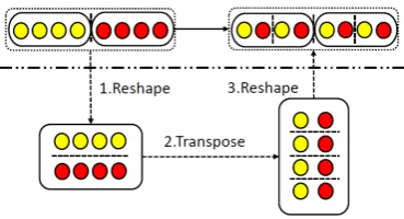
The representation rearrangement layer is parameter-free and simple. We leverage the same implementation in (Zhang et al., 2017b) to con-duct the rearrangement. It’s finished with basic tensor operations reshape, and transpose, which brings (almost) no runtime overhead in our ex-periments. Consider the immediate representation ht ∈ RN outputted by group recurrent layer with group number K. First, we reshape the repre-sentation to add an additional group dimension, resulting in a tensor with new shape (K, N/K). Second, we transpose the two dimensions of the temporary tensor, changing the tensor shape to (N/K, K). Finally, we reshape the tensor along the first axis to restore the representation to its original shape (a vector of sizeN). Figure3 illus-trates the operations with a simple example whose representation is with size 8 and group number is 2.
Combining the group recurrent layer and repsentation rearrangement layer, we rebuild the re-current layer into an efficient and effective layer. We note that, different from convolutional neural networks that are only deep in space, the stack RNNs are deep in both space and time. Figure1
illustrates our architecture along the spatial direc-tion, and Figure2illustrates our architecture along the temporal direction. By applying group op-eration and representation rearrangement in both space and time, we build a new recurrent neural network with high efficiency.
3 Discussion
In this section, we analyze the relation between group recurrent layer and standard recurrent layer, and discuss the advantages of group recurrent net-works.
3.1 Relation to standard recurrent layer
The group recurrent layer in Equation4and5can be re-formulated as
ht= tanh (
W1 0 · · · 0
0 W2 · · · 0
... ... ... ...
0 0 · · · WK
x1t x2t ... xKt
+
U1 0 · · · 0
0 U2 · · · 0 ... ... ... ...
0 0 · · · UK
h1 t h2t ... hKt
) (7)
From the reformulation, we can see group recur-rent layer is equivalent to standard recurrecur-rent layer with block-diagonal sparse weight matrix. Our method employs a group level sparsity in recurrent computation, leading to a uniform sparse struc-ture. This uniform sparse structure can enjoy the efficient computing of dense matrix, as we dis-cussed in Section 2.1. This reformulation also shows that there is no connection across neurons in different groups. Increasing the group number will lead to higher sparse rate. This sparse structure may limit the representation ability of our model. In order to recover the correlation across differ-ent groups, we add represdiffer-entation rearrangemdiffer-ent to make up for representation ability.
3.2 Model capacity
Figure 3: Illustration of the implementation of repre-sentation rearrangement with basic tensor operation.
additional computation and parameter overhead. Given a standard recurrent neural network, we can construct a corresponding group recurrent neural network with same number of parameters, but with K times wider, or withK times deeper. A factor smaller thanK would make our networks still ef-fective than standard recurrent network, but with wider and/or deeper recurrent layers. This could somehow compensate the potential performance drop due to the aggressive sparsity when group number is too large. Therefore, our architecture provides large model space to find a better trade-off between parameter and performance given a fixed resource budget. And our model is a more effective RNN architecture when the network goes deeper and wider.
At last, we note that our architecture focuses on improving the efficiency of recurrent layers. Thus the whole parameter and computational cost re-duction depend on the ratio of recurrent layer in the entire network. Consider a text classification task, a often used RNN model would introduce an embedding layer for the input tokens and a soft-max layer for the output, making the parameter re-duction and speedup for the whole network is not strictly linear with the group number. However, we argue that for deeper and/or wider RNN whose recurrent layers dominate the parameter and com-putational cost, our method would enjoy more ef-ficiency improvement.
4 Experiments
In this section, we present results on three se-quence learning tasks to show the effectiveness of our method: 1). language modeling; 2). neural machine translation; 3). abstractive summariza-tion.
4.1 Language modeling
For evaluating the effectiveness of our approach, we perform language modeling over Penn Tree-bak (PTB) dataset (Marcus et al., 1993). We use the data preprocessed by (Mikolov et al.,
2010) 1, which consists of 929K training words,
73K validation words, and 82K test words. It has 10K words in its vocabulary. We compare our method (named Group LSTM) with the stan-dard LSTM baseline (Zaremba et al., 2014) and its two variants with Bayesian dropout (named LSTM + BD) (Gal and Ghahramani, 2016) and with word tying (named LSTM + WT) (Press and Wolf, 2017). Following the big model settings in (Zaremba et al., 2014; Gal and Ghahramani,
2016; Inan et al., 2016) , all experiments use a two-layer LSTM with1,500hidden units and an embedding of size 1,500. We set group number 2 in this experiment since PTB is a relative sim-ple dataset. We use Stochastic Gradient Descent (SGD) to train all models.
Results We compare the word level perplexity obtained by the standard LSTM baseline mod-els and our group variants, in which we replace the standard LSTM layer with our group LSTM layer. As shown in Table1, Group LSTM achieves comparable performance with the standard LSTM baseline, but with a 27%parameter reduction. A variant using Bayesian dropout (BD) is proposed by (Gal and Ghahramani, 2016) to prevent over-fitting and improve performance. We test our model with LSTM + BD, achieving similar re-sults with above comparison. Finally, we compare our model with the recently proposed word tying (WT) technology, which ties input embedding and output embedding with same weights. Our model achieves even better perplexity than the results re-ported by (Press and Wolf,2017). Since word ty-ing reduces the number of parameters of embed-ding and softmax layers, thus improving the ratio of LSTM layer parameter. Our method achieves a 35%parameter reduction.
4.2 Neural machine translation
We then study our model in neural machine trans-lation. We conduct experiments on two translation tasks, German-English task (De-En for short) and English-German task (En-De for short). For De-En translation, we use data from the De-De-En
Model Parameters Validation Set Test Set
LSTM (Zaremba et al.,2014) 66M 82.2 78.4
2 Group LSTM 48M 82.0 78.6
LSTM + BD (Gal and Ghahramani,2016) 66M 77.9 75.2
2 Group LSTM + BD 48M 79.9 75.8
LSTM + WT (Press and Wolf,2017) 51M 77.4 74.3
2 Group LSTM + WT 33M 76.8 73.3
LSTM + BD + WT (Press and Wolf,2017) 51M 75.8 73.2
[image:6.595.137.460.60.158.2]2 Group LSTM + BD + WT 33M 75.6 71.8
Table 1: Single model complexity on validation and test sets for the Penn Treebank language modeling task. BD is Bayesian dropout. WT is word tying.
chine translation track of the IWSLT 2014 evalua-tion campaign (Cettolo et al.,2014). We follow the pre-processing described in previous works (Wu et al., 2017). The training data comprises about 153K sentence pairs. The size of validation data set is6,969, and the test set is6,750. For En-De translation, we use a widely adopted dataset (Jean et al.,2015;Wu et al.,2016). Specifically, part of data in WMT’14 is used as the training data, which consists of 4.5M sentences pairs. newstest2012
andnewstest2013are concatenated as the valida-tion set andnewstest2014 acts as test set. These two datasets are preprocessed by byte pair encod-ing (BPE) with vocabulary of 25K and30K for De-En and En-De respectively, and the max length of sub-word sentence is64.
Our model is based on RNNSearch model ( Bah-danau et al., 2014), but replacing the standard LSTM layer with our group LSTM layer. There-fore, we name our model as Group RNNSearch model. The model is constructed by LSTM en-coder and deen-coder with attention, where the first layer of encoder is bidirectional LSTM. For De-En, we use two layers for both encoder and de-coder. The embedding size is256, which is same as the hidden size for all LSTM layers. As for En-De, we use four layers for encoder and decoder2.
The embedding size is512and the hidden size is 1024 3. All the models are trained by Adadelta (Zeiler,2012) with initial learning rate 1.0. The gradient is clipped with threshold2.5. The mini-batch size is32for De-En and128for En-De. We use dropout (Srivastava et al.,2014) with rate0.1 for all layers except the layer before softmax with 0.5. We halve the learning rate according to the validation performance.
2For easy to implement, we still keep the first layer with
attention computation in the decoder as original LSTM layer.
3In our implementation, suppose the hidden size isd, after
the first bi-directional LSTM layer in the encoder, the hidden size of the above LSTM layers in the encoder should be2×d.
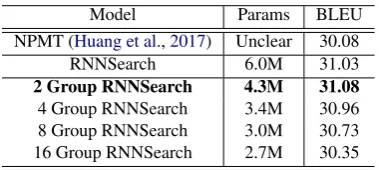
Model Params BLEU
NPMT (Huang et al.,2017) Unclear 30.08
RNNSearch 6.0M 31.03
2 Group RNNSearch 4.3M 31.08
[image:6.595.322.512.206.291.2]4 Group RNNSearch 3.4M 30.96 8 Group RNNSearch 3.0M 30.73 16 Group RNNSearch 2.7M 30.35
Table 2: BLEU scores on IWSLT 2014 De-En test set. We report BLEU score results together with number of parameters of recurrent layers.
Model Params BLEU
DeepLAU (Wang et al.,2017) Unclear 23.80 GNMT (Wu et al.,2016) 160M‡ 24.61
[image:6.595.317.516.345.409.2]2 Group RNNSearch 111M 23.93 4 Group RNNSearch 78M 23.61 Table 3: BLEU scores on WMT’14 En-De test set. We report BLEU score results together with number of pa-rameters of recurrent layers. Numbers with‡ are
ap-proximately calculated by ourselves according to the settings described in the paper.
Results We compute tokenized case-sensitive BLEU (Papineni et al., 2002) 4 score as
evalua-tion metric. For decoding, we use beam search (Sutskever et al.,2014) with beam size5.
From Table 2, we can observe that on De-En task, Group RNNSearch models achieve compa-rable or better BLEU score compared with the RNNSearch but with much less number of param-eters. Specifically, with group number 2 and 4, we achieve about28%and43%parameter reduc-tion of recurrent layers respectively. Note that our results also outperform the state-of-the-art result reported in NPMT (Huang et al.,2017).
The En-De translation results are shown in Table 3. We compare our Group RNNSearch models with Google’s GNMT system (Wu et al.,
2016) and DeepLAU (Wang et al., 2017). Our 4
Group RNNSearch model achieves 23.61, which is comparable to DeepLAU (23.80). Our 2 Group RNNSearch model achieves a BLEU score of 23.93, slightly less than GNMT (24.61), but out-performs the DeepLAU. More importantly, our Group RNNSearch models decrease more than 30%and50%RNN parameters with 2 groups and 4 groups respectively compared with GNMT.
4.3 Abstractive summarization
At last, we valid our approach on abstractive sum-marization task. We train on the Gigaword corpus (Graff and Cieri, 2003) and pre-process it iden-tically to (Rush et al., 2015; Shen et al., 2016), resulting in 3.8M training article-headline pairs, 190K for validation and2,000 for test. Similar to (Shen et al.,2016), we use a source and target vocabulary consisting of30Kwords.
The model is almost same as the one used in De-En machine translation, which is a two lay-ers RNNSearch model, except that the embedding size is512, and the LSTM hidden size in both en-coder and deen-coder is512. The initial values of all weight parameters are uniformly sampled between (−0.05,0.05). We train our Group RNNSearch model by Adadelta (Zeiler, 2012) with learning rate1.0 and gradient clipping threshold1.5(
Pas-canu et al.,2013b). The mini-batch size is64.
Results We evaluate the summarization task by commonly used ROUGE (Lin, 2004) F1 score. During decoding, we use beam search with beam size 10. The results are shown in Table4.
From Table 4, we can observe that the perfor-mance is consistent with machine translation task. Our Group RNNSearch model achieves compa-rable results with RNNSearch, and our 2 Group RNNSearch model even outperforms RNNSearch baseline. Besides, we compare with several other widely adopted methods, our models also show strong performance. Therefore, we can keep the good performance even though we reduce the parameters of the recurrent layers by nearly 50%, which greatly proves the effectiveness of our method.
4.4 Ablation analysis
In addition to showing that group RNN can achieve competing or better performance with much less number of parameters, we further study the effect of group number to training speed and convergence, and the effect of representation
rear-Model Params R-1 R-2 R-L
(Rush et al.,2015) - 29.8 11.9 26.9
(Luong et al.,2015) - 33.1 14.4 30.7
(Chopra et al.,2016) - 33.8 15.9 31.1
RNNSearch 24.1M 34.4 15.8 31.8
2 Group RNNSearch 17.0M 34.8 15.9 32.1
[image:7.595.309.526.62.166.2]4 Group RNNSearch 13.5M 34.3 15.7 31.6 8 Group RNNSearch 11.8M 34.3 15.6 31.6 16 Group RNNSearch 10.9M 33.8 15.3 31.2 Table 4: ROUGE F1 scores on abstractive summariza-tion test set. RG-N stands for N-gram based ROUGE F1 score, RG-L stands for longest common subse-quence based ROUGE F1 score. Params stands for the parameters of the recurrent layers.
Group without with (improvement)
2 82.5 78.6 (+4.7%)
4 86.6 82.6 (+4.6%)
Table 5: The effect of representation rearrangement to model performance.
rangement to performance. Due to space limita-tion, we only report results for language modeling on PTB dataset; for other tasks we have similar results.
In Figure 4, the left one shows that how num-ber of parameters and training speed vary when group number ranging from 1 to 16. We can see that the number of parameters (of recurrent lay-ers) is reduced linearly when increasing number of groups. In the meantime, we also achieves sub-stantial speed up about throughput when increas-ing group number. We note that the speedup is sub-linear instead of linear since our method fo-cuses on the speedup on recurrent layers, as dis-cussed in Section 3.2. Besides, we also com-pare the convergence curve in the right of Figure
4, which shows that our method (almost) doesn’t slow down the convergence in terms of epoch number. Considering the throughput speedup of our method, we can accelerate training by a large margin.
[image:7.595.338.494.249.284.2]20 21 22 23 24 Group number
0 5 10 15 20 25 30 35 40
Number of parameters (M)
Number of parameters
1000 1500 2000 2500 3000 3500 4000 4500
Training speed (WPS)
Training speed
0 5 10 15 20 25 30 35 40
Epoch 50
100 150 200 250
Test perplexity
[image:8.595.111.486.70.210.2]Group number = 1 Group number = 2 Group number = 4
Figure 4: Illustration of group recurrent network analysis. Left: The number of parameters and the training speed (word per second, WPS) on different group numbers. Right: The test perplexity (convergence curve) along the training epochs.
5 Related Work
Improving RNN efficiency for sequence learning is a hot topic in recent deep learning research. For parameter and computation reduction, LightRNN (Li et al.,2016) is proposed to solve big vocabu-lary problem with a 2-component shared embed-ding, while our work addresses the parameter re-dundancy caused by recurrent layers. To speed up RNN, Persistent RNN (Diamos et al.,2016) is pro-posed to improve the RNN computation through-put by mapping deep RNN efficiently onto GPUs, which exploits GPU’s inverted memory hierarchy to reuse network weights over multiple time steps. (Neil et al.,2017) proposes delta networks for op-timizing the matrix-vector multiplications in RNN computation by considering the temporal proper-ties of the data. Quasi-RNN (Bradbury et al.,
2016) and SRU (Lei and Zhang, 2017) are pro-posed for speeding up RNN computation by de-signing novel recurrent units which relax depen-dency between time steps. Different from these works, we optimize RNN from the perspective of network architecture innovation by adopting a group strategy.
There is a long history about the group idea in deep learning, especially in convolutional neu-ral networks, aiming to improve the computation efficiency and parameter efficiency. Such works can date back at least to AlexNet (Krizhevsky et al., 2012), which splits the convolutional lay-ers into 2 independent groups for the ease of model-parallelism. The Inception (Szegedy et al.,
2015) architecture proposes a module that em-ploys uniform sparsity to improve the parameter efficiency. Going to the extreme of Inception, the
Xception (Chollet,2016) adopts a depthwise sep-arable convolution, where each spatial convolu-tion only works on a single channel. MobileNet (Howard et al.,2017) uses the same idea for effi-cient mobile model. IGCNet (Zhang et al.,2017a) and ShuffleNet (Zhang et al., 2017b) also adopt the group convolution idea, and further permute the features across consecutive layers. Similar to these works, we also exploit the group strategy. But we focus on efficient sequence learning with RNN, which, different from CNN, contains an in-ternal memory and an additional temporal direc-tion. In the RNN literature, there is only one paper (Kuchaiev and Ginsburg,2017), to our best knowl-edge, exploiting the group strategy. However, this work assumes the features are group independent, thus failing to capturing the inter-group correla-tion. Our work employs a representational rear-rangement mechanism, which avoids the assump-tion and improves the performance, as shown in our empirical experiments.
6 Conclusion
References
Dzmitry Bahdanau, Kyunghyun Cho, and Yoshua Ben-gio. 2014. Neural machine translation by jointly learning to align and translate. arXiv preprint arXiv:1409.0473.
James Bradbury, Stephen Merity, Caiming Xiong, and Richard Socher. 2016. Quasi-recurrent neural net-works. arXiv preprint arXiv:1611.01576.
Mauro Cettolo, Jan Niehues, Sebastian St¨uker, Luisa Bentivogli, and Marcello Federico. 2014. Report on the 11th iwslt evaluation campaign, iwslt 2014.
Franc¸ois Chollet. 2016. Xception: Deep learning with depthwise separable convolutions. arXiv preprint arXiv:1610.02357.
Sumit Chopra, Michael Auli, and Alexander M Rush. 2016. Abstractive sentence summarization with at-tentive recurrent neural networks. InNAACL. pages 93–98.
Greg Diamos, Shubho Sengupta, Bryan Catanzaro, Mike Chrzanowski, Adam Coates, Erich Elsen, Jesse Engel, Awni Hannun, and Sanjeev Satheesh. 2016. Persistent rnns: Stashing recurrent weights on-chip. In International Conference on Machine Learning. pages 2024–2033.
Yarin Gal and Zoubin Ghahramani. 2016. A theoret-ically grounded application of dropout in recurrent neural networks. InAdvances in neural information processing systems. pages 1019–1027.
David Graff and C Cieri. 2003. English gigaword, lin-guistic data consortium.
Alex Graves, Abdel-rahman Mohamed, and Geoffrey Hinton. 2013. Speech recognition with deep recur-rent neural networks. InAcoustics, speech and sig-nal processing (icassp), 2013 ieee internatiosig-nal con-ference on. IEEE, pages 6645–6649.
Andrew G Howard, Menglong Zhu, Bo Chen, Dmitry Kalenichenko, Weijun Wang, Tobias Weyand, Marco Andreetto, and Hartwig Adam. 2017. Mo-bilenets: Efficient convolutional neural networks for mobile vision applications. arXiv preprint arXiv:1704.04861.
Po-Sen Huang, Chong Wang, Dengyong Zhou, and Li Deng. 2017. Neural phrase-based machine trans-lation. CoRRabs/1706.05565.
Hakan Inan, Khashayar Khosravi, and Richard Socher. 2016. Tying word vectors and word classifiers: A loss framework for language modeling. arXiv preprint arXiv:1611.01462.
S´ebastien Jean, Kyunghyun Cho, Roland Memisevic, and Yoshua Bengio. 2015. On using very large tar-get vocabulary for neural machine translation. In
ACL.
Yoon Kim and Alexander M. Rush. 2016. Sequence-level knowledge distillation. InProceedings of the 2016 Conference on Empirical Methods in Natu-ral Language Processing. Association for Compu-tational Linguistics, pages 1317–1327.
Alex Krizhevsky, Ilya Sutskever, and Geoffrey E Hin-ton. 2012. Imagenet classification with deep con-volutional neural networks. In Advances in neural information processing systems. pages 1097–1105.
Oleksii Kuchaiev and Boris Ginsburg. 2017. Factor-ization tricks for lstm networks. arXiv preprint arXiv:1703.10722.
Tao Lei and Yu Zhang. 2017. Training rnns as fast as cnns. arXiv preprint arXiv:1709.02755.
Xiang Li, Tao Qin, Jian Yang, Xiaolin Hu, and Tieyan Liu. 2016. Lightrnn: Memory and computation-efficient recurrent neural networks. In D. D. Lee, M. Sugiyama, U. V. Luxburg, I. Guyon, and R. Gar-nett, editors, Advances in Neural Information Pro-cessing Systems 29, Curran Associates, Inc., pages 4385–4393.
Chin-Yew Lin. 2004. Rouge: A package for auto-matic evaluation of summaries. In ACL-04 work-shop. Barcelona, Spain.
Minh-Thang Luong, Hieu Pham, and Christopher D Manning. 2015. Effective approaches to attention-based neural machine translation. InEMNLP.
Mitchell P Marcus, Mary Ann Marcinkiewicz, and Beatrice Santorini. 1993. Building a large annotated corpus of english: The penn treebank. Computa-tional linguistics19(2):313–330.
Stephen Merity, Nitish Shirish Keskar, and Richard Socher. 2017. Regularizing and Optimiz-ing LSTM Language Models. arXiv preprint arXiv:1708.02182.
Tomas Mikolov, Martin Karafit, Lukas Burget, Jan Cernock, and Sanjeev Khudanpur. 2010. Recur-rent neural network based language model. In IN-TERSPEECH 2010, Conference of the International Speech Communication Association, Makuhari, Chiba, Japan, September. pages 1045–1048.
Daniel Neil, Jun Haeng Lee, Tobi Delbruck, and Shih-Chii Liu. 2017. Delta networks for optimized re-current network computation. In Doina Precup and Yee Whye Teh, editors, Proceedings of the 34th International Conference on Machine Learn-ing. PMLR, International Convention Centre, Syd-ney, Australia, volume 70 of Proceedings of Ma-chine Learning Research, pages 2584–2593.
Razvan Pascanu, Caglar Gulcehre, Kyunghyun Cho, and Yoshua Bengio. 2013a. How to construct deep recurrent neural networks. arXiv preprint arXiv:1312.6026.
Razvan Pascanu, Tomas Mikolov, and Yoshua Bengio. 2013b. On the difficulty of training recurrent neural networks. InICML. pages 1310–1318.
Ofir Press and Lior Wolf. 2017. Using the output em-bedding to improve language models. In Proceed-ings of the 15th Conference of the European Chap-ter of the Association for Computational Linguistics: Volume 2, Short Papers. Association for Computa-tional Linguistics, Valencia, Spain, pages 157–163. Alexander M Rush, Sumit Chopra, and Jason
We-ston. 2015. A neural attention model for ab-stractive sentence summarization. arXiv preprint arXiv:1509.00685.
Shiqi Shen, Yu Zhao, Zhiyuan Liu, Maosong Sun, et al. 2016. Neural headline generation with sentence-wise optimization. arXiv preprint arXiv:1604.01904.
Nitish Srivastava, Geoffrey E Hinton, Alex Krizhevsky, Ilya Sutskever, and Ruslan Salakhutdinov. 2014. Dropout: a simple way to prevent neural networks from overfitting. Journal of machine learning re-search15(1):1929–1958.
Ilya Sutskever, Oriol Vinyals, and Quoc V Le. 2014. Sequence to sequence learning with neural net-works. InAdvances in neural information process-ing systems. pages 3104–3112.
Christian Szegedy, Wei Liu, Yangqing Jia, Pierre Sermanet, Scott Reed, Dragomir Anguelov, Du-mitru Erhan, Vincent Vanhoucke, and Andrew Ra-binovich. 2015. Going deeper with convolutions. In
Proceedings of the IEEE conference on computer vi-sion and pattern recognition. pages 1–9.
Mingxuan Wang, Zhengdong Lu, Jie Zhou, and Qun Liu. 2017. Deep neural machine transla-tion with linear associative unit. arXiv preprint arXiv:1705.00861.
Lijun Wu, Li Zhao, Tao Qin, Jianhuang Lai, and Tie-Yan Liu. 2017. Sequence prediction with unlabeled data by reward function learning. InProceedings of the Twenty-Sixth International Joint Conference on Artificial Intelligence, IJCAI-17. pages 3098–3104. Yonghui Wu, Mike Schuster, Zhifeng Chen, Quoc V
Le, Mohammad Norouzi, Wolfgang Macherey, Maxim Krikun, Yuan Cao, Qin Gao, Klaus Macherey, et al. 2016. Google’s neural ma-chine translation system: Bridging the gap between human and machine translation. arXiv preprint arXiv:1609.08144.
Wojciech Zaremba, Ilya Sutskever, and Oriol Vinyals. 2014. Recurrent neural network regularization.
arXiv preprint arXiv:1409.2329.
Matthew D Zeiler. 2012. Adadelta: an adaptive learn-ing rate method.arXiv preprint arXiv:1212.5701.
Ting Zhang, Guo-Jun Qi, Bin Xiao, and Jing-dong Wang. 2017a. Primal-dual group convolu-tions for deep neural networks. arXiv preprint arXiv:1707.02725.