A fast finite state relaxation method for enforcing global constraints on sequence decoding

(1)

A fast finite-state relaxation method for enforcing

global constraints on sequence decoding

Roy W. Tromble and Jason Eisner

Department of Computer Science and Center for Language and Speech Processing Johns Hopkins University

Baltimore, MD 21218 {royt,jason}@cs.jhu.edu

Abstract

We describe finite-state constraint relaxation, a method for ap-plying global constraints, expressed as automata, to sequence model decoding. We present algorithms for both hard con-straints and binary soft concon-straints. On the CoNLL-2004 se-mantic role labeling task, we report a speedup of at least 16x over a previous method that used integer linear programming.

1 Introduction

Many tasks in natural language processing involve sequence labeling. If one models long-distance or global properties of labeled sequences, it can be-come intractable to find (“decode”) the best labeling of an unlabeled sequence.

Nonetheless, such global properties can improve the accuracy of a model, so recent NLP papers have considered practical techniques for decod-ing with them. Such techniques include Gibbs sampling (Finkel et al., 2005), a general-purpose Monte Carlo method, and integer linear program-ming (ILP), (Roth and Yih, 2005), a general-purpose exact framework for NP-complete problems.

Under generative models such as hidden Markov models, the probability of a labeled sequence de-pends only on its local properties. The situation improves with discriminatively trained models, such as conditional random fields (Lafferty et al., 2001), which do efficiently allow features that are functions of the entire observation sequence. However, these features can still only look locally at the label se-quence. That is a significant shortcoming, because in many domains, hard or soft global constraints on the label sequence are motivated by common sense:

• For named entity recognition, a phrase that appears multiple times should tend to get the same label each time (Finkel et al., 2005).

• In bibliography entries (Peng and McCallum, 2004), a given field (author, title, etc.) should

be filled by at most one substring of the in-put, and there are strong preferences on the co-occurrence and order of certain fields.

• In seminar announcements, a given field (speaker, start time, etc.) should appear with at most one value in each announcement, al-though the field and value may be repeated (Finkel et al., 2005).

• For semantic role labeling, each argument should be instantiated only once for a given verb. There are several other constraints that we will describe later (Roth and Yih, 2005).

A popular approximate technique is to hypothe-size a list of possible answers by decoding without any global constraints, and then rerank (or prune) this n-best list using the full model with all con-straints. Reranking relies on the local model being “good enough” that the globally best answer appears in itsn-best list. Otherwise, reranking can’t find it.

In this paper, we propose “constraint relaxation,” a simple exact alternative to reranking. As in rerank-ing, we start with a weighted lattice of hypotheses proposed by the local model. But rather than restrict to thenbest of these according to the local model, we aim to directly extract the one best according to the global model. As in reranking, we hope that the local constraints alone will work well, but if they do not, the penalty is not incorrect decoding, but longer runtime as we gradually fold the global constraints into the lattice. Constraint relaxation can be used whenever the global constraints can be expressed as regular languages over the label sequence.

In the worst case, our runtime may be exponential in the number of constraints, since we are consider-ing an intractable class of problems. However, we show that in practice, the method is quite effective at rapid decoding under global hard constraints.

(2)

0 O

1 ?

O ?

Figure 1: An automaton expressing the constraint that the label sequence cannot beO∗. Here?matches any symbol exceptO.

The remainder of the paper is organized as fol-lows: In §2 we describe how finite-state automata can be used to apply global constraints. We then give a brute-force decoding algorithm (§3). In §4, we present a more efficient algorithm for the case of hard constraints. We report results for the semantic role labeling task in§5.§6 treats soft constraints.

2 Finite-state constraints

Previous approaches to global sequence labeling— Gibbs sampling, ILP, and reranking—seem moti-vated by the idea that standard sequence methods are incapable of considering global constraints at all.

In fact, finite-state automata (FSAs) are powerful enough to express many long-distance constraints. Since all finite languages are regular, any constraint over label sequences of bounded length is finite-state. FSAs are more powerful than n-gram mod-els. For example, the regular expressionΣ∗XΣ∗YΣ∗

matches only sequences of labels that contain an X

before aY. Similarly, the regular expression¬(O∗)

requires at least one non-Olabel; it compiles into the FSA of Figure 1.

Note that this FSA is in one or the other of its two states according to whether it has encountered a

non-Olabel yet. In general, the current state of an FSA records properties of the label sequence prefix read so far. The FSA needs enough states to keep track of whether the label sequence as a whole satisfies the global constraint in question.

FSAs are a flexible approach to constraints be-cause they are closed under logical operations such as disjunction (union) and conjunction (intersec-tion). They may be specified by regular expressions (Karttunen et al., 1996), in a logical language (Vail-lette, 2004), or directly as FSAs. They may also be weighted to express soft constraints.

Formally, we pose the decoding problem in terms of an observation sequencex∈ X∗_{and possible}

la-bel sequencesy∈ Y∗. In many NLP tasks,X is the set of words, andY the tags. A latticeL: Y∗ _7→

R maps label sequences to weights, and is encoded as a weighted FSA. Constraints are formally the same— any function C: Y∗ _7→

R is a constraint, includ-ing weighted features from a classifier or probabilis-tic model. In this paper we will consider only con-straints that are weighted in particular ways.

Given a latticeLand constraintsC, we seek

y∗def= argmax

y

L(y) +X

C∈C

C(y) !

. (1)

We assume the latticeLis generated by a model M: X∗ _7→ ₍_Y∗ _7→

R). For a given observation se-quencex, we putL = M(x). One possible model is a finite-state transducer, where M(x) is an FSA found by composing the transducer withx. Another is a CRF, whereM(x)is a lattice with sums of log-potentials for arc weights.1

3 A brute-force finite-state decoder

To find the best constrained labeling in a lattice,y∗, according to (1), we could simply intersect the lat-tice with all the constraints, then extract the best path.

Weighted FSA intersection is a generalization of ordinary unweighted FSA intersection (Mohri et al., 1996). It is customary in NLP to use the so-called tropical semiring, where weights are represented by their natural logarithms and summed rather than multiplied. Then the intersected automatonL∩C computes

(L∩C)(y)def= L(y) +C(y) (2)

To find y∗, one would extract the best path in L∩C1 ∩C2 ∩ · · · using the Viterbi algorithm, or

Dijkstra’s algorithm if the lattice is cyclic. This step is fast if the intersected automaton is small.

The problem is that the multiple intersections in L∩C1∩C2∩ · · ·can quickly lead to an FSA with

an intractable number of states. The intersection of two finite-state automata produces an automaton

1

For example, ifM is a simple linear-chain CRF,L(y) =

Pn

i=1f(yi−1, yi) +g(xi, yi). We buildL = M(x) as an

(3)

with the cross product state set. That is, ifF hasm states andGhasnstates, thenF∩Ghas up tomn states (fewer if some of the mn possible states do not lie on any accepting path).

Intersection of many such constraints, even if they have only a few states each, quickly leads to a com-binatorial explosion. In the worst case, the size, in states, of the resulting lattice is exponential in the number of constraints. To deal with this, we present a constraint relaxation algorithm.

4 Hard constraints

The simplest kind of constraint is the hard con-straint. Hard constraints are necessarily binary— either the labeling satisfies the constraint, or it vi-olates it. Violation is fatal—the labeling produced by decoding must satisfy each hard constraint.

Formally, a hard constraint is a mappingC:Y∗ 7→ {0,−∞}, encoded as an unweighted FSA. If a string satisfies the constraint, recognition of the string will lead to an accepting state. If it violates the con-straint, recognition will end in a non-accepting state. Here we give an algorithm for decoding with a set of such constraints. Later (§6), we discuss the case of binary soft constraints. In what follows, we will assume that there is always at least one path in the lattice that satisfies all of the constraints.

4.1 Decoding by constraint relaxation

Our decoding algorithm first relaxes the global con-straints and solves a simpler problem. In particular, we find the best labeling according to the model,

y∗₀ def= argmax

y

L(y) (3)

ignoring all the constraints inC.

Next, we check whether y∗₀ satisifies the con-straints. If so, then we are done—y∗₀ is also y∗. If not, then we reintroduce the constraints. However, rather than include all at once, we introduce them only as they are violated by successive solutions to the relaxed problems:y∗₀,y∗₁, etc. We define

y∗₁ def= argmax

y

(L(y) +C(y)) (4)

for some constraint C thaty₀∗ violates. Similarly,

y∗₂satisfies an additional constraint thaty∗₁violates,

HARD-CONSTRAIN-LATTICE(L,C): 1. y:=Best-Path(L)

2. while∃C∈ Csuch thatC(y) =−∞: 3. L:=L∩C

4. C:=C − {C} 5. y:=Best-Path(L) 6. returny

Figure 2: Hard constraints decoding algorithm.

and so on. Eventually, we find somekfor whichy_k∗

satisfies all constraints, and this path is returned. To determine whether a labelingysatisfies a con-straintC, we represent yas a straight-line automa-ton and intersect withC, checking the result for non-emptiness. This is equivalent to string recognition.

Our hope is that, although intractable in the worst case, the constraint relaxation algorithm will operate efficiently in practice. The success of traditional se-quence models on NLP tasks suggests that, for nat-ural language, much of the correct analysis can be recovered from local features and constraints alone. We suspect that, as a result, global constraints will often be easy to satisfy.

Pseudocode for the algorithm appears in Figure 2. Note that line 2 does not specify how to choose C from among multiple violated constraints. This is discussed in §7. Our algorithm resembles the method of Koskenniemi (1990) and later work. The difference is that there lattices are unweighted and may not contain a path that satisfies all constraints, so that the order of constraint intersection matters.

5 Semantic role labeling

The semantic role labeling task (Carreras and M`arques, 2004) involves choosing instantiations of verb arguments from a sentence for a given verb. The verb and its arguments form a proposition. We use data from the CoNLL-2004 shared task—the PropBank (Palmer et al., 2005) annotations of the Penn Treebank (Marcus et al., 1993), with sections 15–18 as the training set and section 20 as the de-velopment set. Unless otherwise specified, all mea-surements are made on the development set.

(4)

(a) 0

?

1 A0

A0

2 ?

?

(b)

0 1

O

A0

A1 A2 A3 A4 A5

2 O

(verb position) A1 A2 A3 A4 A5

O A0

(c) 0

[image:4.612.77.291.57.204.2]

O A0 A1 A2 A3

Figure 4: Automata expressing NO DUPLICATEA0(?matches anything butA0), KNOWN VERB POSITION[2], and DISALLOW ARGUMENTS[A4,A5].

adjuncts and references asO.

Figure 3 shows an example sentence from the shared task. It is marked with an IOB phrase chunk-ing, the heads of the phrases, and the correct seman-tic role labeling. Heads are taken to be the rightmost words of chunks. On average, there are 18.8 phrases per proposition, vs. 23.5 words per sentence. Sen-tences may contain multiple propositions. There are 4305 propositions in section 20.

5.1 Constraints

Roth and Yih use five global constraints on label se-quences for the semantic role labeling task. We ex-press these constraints as FSAs. The first two are general, and the seven automata encoding them can be constructed offline:

• NO DUPLICATE ARGUMENT LABELS

(Fig. 4(a)) requires that each verb have at most one argument of each type in a given sentence. We separate this into six individual constraints, one for each core argument type. Thus, we have constraints called NO DUPLI -CATE A0, NO DUPLICATE A1, etc. Each of these is represented as a three-state FSA.

• AT LEAST ONE ARGUMENT(Fig. 1) simply

re-quires that the label sequence is notO∗. This is a two-state automaton as described in§2.

The last three constraints require information about the example, and the automata must be con-structed on a per-example basis:

• ARGUMENT CANDIDATES (Fig. 5) encodes a set of position spans each of which must re-ceive only a single label type. These spans were proposed using a high-recall heuristic (Xue and Palmer, 2004).

• KNOWN VERB POSITION (Fig. 4(b)) simply encodes the position of the verb in question, which must be labeledO.

• DISALLOW ARGUMENTS(Fig. 4(c)) specifies argument types that are compatible with the verb in question, according to PropBank.

5.2 Experiments

We implemented our hard constraint relaxation al-gorithm, using the FSA toolkit (Kanthak and Ney, 2004) for finite-state operations. FSA is an open-source C++ library providing a useful set of algo-rithms on weighted finite-state acceptors and trans-ducers. For each example we decoded, we chose a random order in which to apply the constraints.

Lattices are generated from what amounts to a unigram model—the voted perceptron classifier of Roth and Yih. The features used are a subset of those commonly applied to the task.

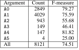
Our system produces output identical to that of Roth and Yih. Table 1 shows F-measure on the core arguments. Table 2 shows a runtime comparison. The ILP runtime was provided by the authors (per-sonal communication). Because the systems were run under different conditions, the times are not di-rectly comparable. However, constraint relaxation is more than sixteen times faster than ILP despite run-ning on a slower platform.

5.2.1 Comparison to an ILP solver

Roth and Yih’s linear program has two kinds of numeric constraints. Some encode the shortest path problem structure; the others encode the global con-straints of §5.1. The ILP solver works by relaxing to a (real-valued) linear program, which may obtain a fractional solution that represents a path mixture instead of a path. It then uses branch-and-bound to seek the optimal rounding of this fractional solution to an integer solution (Gu´eret et al., 2002) that repre-sents a single path satisfying the global constraints.

(5)

Mr. Turner said the test will be shipped in 45 days to hospitals and clinical laboratories .

B-NP I-NP B-VP B-NP I-NP B-VP I-VP I-VP B-PP B-NP I-NP B-PP B-NP O B-NP I-NP O

Turner said test shipped in days to hospitals and laboratories .

[image:5.612.72.538.58.104.2]

A0 O A1 A1 A1 A1 A1 A1 A1 A1 O

Figure 3: Example sentence, with phrase tags and heads, and core argument labels. TheA1argument of “said” is a long clause.

0 1 O A0 A1 A2 A3 A4 A5 2 A2 A3 A4 A5 O A0 A1 4 O 10 A0 16 A1 22 A2 28 A3 34 A4 40 A5 5 O 11 A0 17 A1 23 A2 29 A3 35 A4 41

A5 A5 ₄₂ A5 ₄₃ A5 ₄₄ A5 ₄₅

3 A5 46 O A0 A1 A2 A3 A4 A5 O A0 A1 A2 A3 A4 A5 36 A4 37 A4 38 A4 39 A4 A4 30

A3 A3 ₃₁ A3 ₃₂ A3 ₃₃ A3 24

A2 A2 ₂₅ A2 ₂₆ A2 ₂₇ A2 18

A1 A1 ₁₉ A1 ₂₀

21 A1

A1 12

A0 A0 ₁₃ A0 ₁₄

15 A0

A0 6

O O ₇ O ₈

9 O

O

Figure 5: An automaton expressing ARGUMENT CANDIDATES.

Argument Count F-measure

A0 2849 79.27

A1 4029 75.59

A2 943 55.68

A3 149 46.41

A4 147 81.82

A5 4 25.00

[image:5.612.75.535.135.252.2]

All 8121 74.51

Table 1: F-measure on core arguments.

satisfies or violates each global constraint. In effect, we are using two kinds of domain knowledge. First, we recognize that this is a graph problem, and insist on true paths so we can use Viterbi decoding. Sec-ond, we choose to relax only domain-specific con-straints that are likely to be satisfied anyway (in our domain), in contrast to the meta-constraint of inte-grality relaxed by ILP. Thus it is cheaper on aver-age for us to repair a relaxed solution. (Our repair strategy—finite-state intersection in place of branch-and-bound search—remains expensive in the worst case, as the problem is NP-hard.)

5.2.2 Constraint violations

The y₀∗s, generated with only local information, satisfy most of the global constraints most of the time. Table 3 shows the violations by type.

The majority of best labelings according to the local model don’t violate any global constraints— a fact especially remarkable because there are no label sequence features in Roth and Yih’s unigram

Constraint Violations Fraction

ARGUMENT CANDIDATES 1619 0.376

NO DUPLICATEA1 899 0.209

AT LEAST ONE ARGUMENT 108 0.025 DISALLOW ARGUMENTS 48 0.011

[image:5.612.323.531.293.406.2]

KNOWN VERB POSITION 0 0.000

Table 3: Violations of constraints byy∗0.

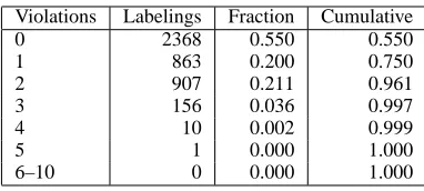
model. This confirms our intuition that natural lan-guage structure is largely apparent locally. Table 4 shows the breakdown. The majority of examples are very efficient to decode, because they don’t require intersection of the lattice with any constraints—y∗₀

is extracted and is good enough. Those examples where constraints are violated are still relatively effi-cient because they only require a small number of in-tersections. In total, the average number of intersec-tions needed, even with the naive randomized con-straint ordering, was only 0.65. The order doesn’t matter very much, since 75% of examples have one violation or fewer.

5.2.3 Effects on lattice size

[image:5.612.119.254.294.379.2]

(6)

con-Method Total Time Per Example Platform

Brute Force Finite-State 37m25.290s 0.522s Pentium III, 1.0 GHz

ILP 11m39.220s 0.162s Xeon, 3.x GHz

[image:6.612.156.454.56.101.2]

Constraint Relaxation 39.700s 0.009s Pentium III, 1.0 GHz Table 2: A comparison of runtimes for constrained decoding with ILP and FSA.

Violations Labelings Fraction Cumulative

0 2368 0.550 0.550

1 863 0.200 0.750

2 907 0.211 0.961

3 156 0.036 0.997

4 10 0.002 0.999

5 1 0.000 1.000

[image:6.612.89.280.140.226.2]

6–10 0 0.000 1.000

Table 4: Number ofy∗0with each violation count.

0 500 1000 1500 2000 2500

0 1 2 3 4 5

Verbs Mean Arcs with Relaxation Mean Arcs with Brute Force

Figure 6: Mean lattice size (measured in arcs) throughout de-coding. Vertical bars show the number of examples over which each mean is computed.

straint relaxation had to intersect k contraints (i.e.,

y∗ ≡ y∗_k). The trajectory ending at (for example) k = 3shows how the average lattice size for that subset of examples evolved over the3intersections. TheXatk= 3shows the final size of the brute-force lattice on the same subset of examples.

For the most part, our lattices do stay much smaller than those produced by the brute-force algo-rithm. (The uppermost curve,k = 5, is an obvious exception; however, that curve describes only the seven hardest examples.) Note that plotting only the final size of the brute-force lattice obscures the long trajectory of its construction, which involves 10 in-tersections and, like the trajectories shown, includes larger intermediate automata.2 This explains the far

2

The final brute-force lattice is especially shrunk by its

in-Constraint Violations Fraction

ARGUMENT CANDIDATES 90 0.0209 AT LEAST ONE ARGUMENT 27 0.0063

Table 5: Violations of constraints byyˆ, measured over the de-velopment set.

longer runtime of the brute-force method (Table 2). Harder examples (corresponding to longer trajec-tories) have larger lattices, on average. This is partly just because it is disproportionately the longer sen-tences that are hard: they have more opportunities for a relaxed decoding to violate global constraints.

Hard examples are rare. The left three columns, requiring only 0–2 intersections, constitute 96% of examples. The vast majority can be decoded without much more than doubling the local-lattice size.

6 Soft constraints

The gold standard labelsyˆ occasionally violate the hard global constraints that we are using. Counts for the development set appear in Table 5. Counts for violations of NO DUPLICATE A·do not include discontinous arguments, of which there are 104 in-stances, since we ignore them.

Because of the infrequency, the hard constraints still help most of the time. However, on a small sub-set of the examples, they preclude us from inferring the correct labeling.

We can apply these constraints with weights, rather than making them inviolable. This constitutes a transition from hard to soft constraints. Formally, a soft constraintC:Y∗ 7→ _R−is a mapping from a label sequence to a non-positive penalty.

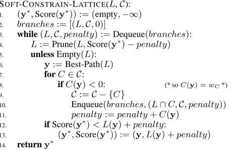
Soft constraints present new difficulty for

[image:6.612.320.532.140.225.2] [image:6.612.81.293.263.421.2]

(7)

SOFT-CONSTRAIN-LATTICE(L,C): 1. (y∗,Score(y∗)) := (empty,−∞) 2. branches:= [(L,C,0)]

3. while(L,C, penalty) :=Dequeue(branches): 4. L:=Prune(L,Score(y∗)−penalty) 5. unless Empty(L):

6. y:=Best-Path(L) 7. forC∈ C:

8. ifC(y)<0: (*soC(y) =wC*)

9. C:=C − {C}

10. Enqueue(branches,(L∩C,C, penalty)) 11. penalty:=penalty+C(y)

12. if Score(y∗)< L(y) +penalty:

[image:7.612.73.302.58.207.2]

13. (y∗,Score(y∗)) := (y, L(y) +penalty) 14. returny∗

Figure 7: Soft constraints decoding algorithm

ing, because instead of eliminating paths ofLfrom contention, they just reweight them.

In what follows, we consider only binary soft constraints—they are either satisfied or violated, and the same penalty is assessed whenever a violation occurs. That is, ∀C ∈ C,∃wC < 0 such that

∀y, C(y)∈ {0, wC}.

6.1 Soft constraint relaxation

The decoding algorithm for soft constraints is a gen-eralization of that for hard constraints. The differ-ence is that, whereas with hard constraints a vio-lation meant disqualification, here viovio-lation simply means a penalty. We therefore must find and com-pare two labelings: the best that satisfies the con-straint, and the best that violates it.

We present a branch-and-bound algorithm (Lawler and Wood, 1966), with pseudocode in Figure 7. At line 9, we process and eliminate a currently violated constraintC ∈ Cby considering two cases. On the first branch, we insist that C be satisfied, enqueuingL∩Cfor later exploration. On the second branch, we assumeC is violated by all paths, and so continue considering L unmodified, but accept a penalty for doing so; we immediately explore the second branch by returning to the start of the for loop.3

Not every branch needs to be completely ex-plored. Bounding is handled by the PRUNE func-tion at line 4, which shrinks L by removing some

3

It is possible that a future best path on the second branch will not actually violateC, in which case we have overpenalized it, but in that case we will also find it with correct penalty on the first branch.

or all paths that cannot score better than Score(y∗), the score of the best path found on any branch so far. Our experiments used almost the simplest possi-ble PRUNE: replaceLby the empty lattice if the best path falls below the bound, else leaveLunchanged.4 A similar bounding would be possible in the im-plicit branches. If, during the for loop, we find that the test at line 12 would fail, we can quit the for loop and immediately move to the next branch in the queue at line 3.

There are two factors in this algorithm that con-tribute to avoiding consideration of all of the expo-nential number of leaves corresponding to the power set of constraints. First, bounding stops evaluation of subtrees. Second, only violated constraints re-quire branching. If a lattice’s best path satisifies a constraint, then the best path that violates it can be no better since, by assumption,∀y, C(y)≤0.

6.2 Runtime experiments

Using the ten constraints from §5.1, weighted naively by their log odds of violation, the soft con-straint relaxation algorithm runs in a time of 58.40 seconds. It is, as expected, slower than hard con-straint relaxation, but only by a factor of about two.

As a side note, softening these particular con-straints in this particular way did not improve de-coding quality in this case. It might help to jointly train the relative weights of these constraints and the local model—e.g., using a perceptron algorithm (Freund and Schapire, 1998), which repeatedly ex-tracts the best global path (using our algorithm), compares it to the gold standard, and adjusts the con-straint weights. An obvious alternative is maximum-entropy training, but the partition function would have to be computed using the large brute-force lat-tices, or else approximated by a sampling method.

7 Future work

For a given task, we may be able to obtain further speedups by carefully choosing the order in which to test and apply the constraints. We might treat this as a reinforcement learning problem (Sutton, 1988),

4

(8)

where an agent will obtain rewards by finding y∗

quickly. In the hard-constraint algorithm, for ex-ample, the agent’s possible moves are to test some constraint for violation by the current best path, or to intersect some constraint with the current lattice. Several features can help the agent choose the next move. How large is the current lattice, which con-straints does it already incorporate, and which re-maining constraints are already known to be satis-fied or violated by its best path? And what were the answers to those questions at previous stages?

Our constraint relaxation method should be tested on problems other than semantic role labeling. For example, information extraction from bibliography entries, as discussed in§1, has about 13 fields to ex-tract, and interesting hard and soft global constraints on co-occurrence, order, and adjacency. The method should also be evaluated on a task with longer se-quences: though the finite-state operations we use do scale up linearly with the sequence length, longer sequences have more chance of violating a global constraint somewhere in the sequence, requiring us to apply that constraint explicitly.

8 Conclusion

Roth and Yih (2005) showed that global constraints can improve the output of sequence labeling models for semantic role labeling. In general, decoding un-der such constraints is NP-complete. We exhibited a practical approach, finite-state constraint relax-ation, that greatly sped up decoding on this NLP task by using familiar finite-state operations—weighted FSA intersection and best-path extraction—rather than integer linear programming.

We have also given a constraint relaxation algo-rithm for binary soft constraints. This allows incor-poration of constraints akin to reranking features, in addition to inviolable constraints.

Acknowledgments

This material is based upon work supported by the National Science Foundation under Grant No. 0347822. We thank Scott Yih for kindly providing both the voted-perceptron classifier and runtime re-sults for decoding with ILP, and the reviewers for helpful comments.

References

Xavier Carreras and Llu´ıs M`arques. 2004. Introduction to the CoNLL-2004 shared task: Semantic role labeling. In Proc.

of CoNLL, pp. 89–97.

Jenny Rose Finkel, Trond Grenager, and Christopher Manning. 2005. Incorporating non-local information into information extraction systems by Gibbs sampling. In Proc. of ACL, pp. 363–370.

Yoav Freund and Robert E. Schapire. 1998. Large margin clas-sification using the perceptron algorithm. In Proc. of COLT, pp. 209–217, New York. ACM Press.

Christelle Gu´eret, Christian Prins, and Marc Sevaux. 2002.

Ap-plications of optimization with Xpress-MP. Dash

Optimiza-tion. Translated and revised by Susanne Heipcke.

Kadri Hacioglu, Sameer Pradhan, Wayne Ward, James H. Mar-tin, and Daniel Jurafsky. 2004. Semantic role labeling by tagging syntactic chunks. In Proc. of CoNLL, pp. 110–113. Stephan Kanthak and Hermann Ney. 2004. FSA: An efficient

and flexible C++ toolkit for finite state automata using on-demand computation. In Proc. of ACL, pp. 510–517. Lauri Karttunen, Jean-Pierre Chanod, Gregory Grefenstette,

and Anne Schiller. 1996. Regular expressions for lan-guage engineering. Journal of Natural Lanlan-guage

Engineer-ing, 2(4):305–328.

Kimmo Koskenniemi. 1990. Finite-state parsing and disam-biguation. In Proc. of COLING, pp. 229–232.

John Lafferty, Andrew McCallum, and Fernando Pereira. 2001. Conditional random fields: Probabilistic models for seg-menting and labeling sequence data. In Proc. of ICML, pp. 282–289.

Eugene L. Lawler and David E. Wood. 1966. Branch-and-bound methods: A survey. Operations Research, 14(4):699– 719.

Mitchell P. Marcus, Beatrice Santorini, and Mary Ann Marcinkiewicz. 1993. Building a large annotated corpus of English: the Penn Treebank. Computational Linguistics, 19:313–330.

Mehryar Mohri, Fernando Pereira, and Michael Riley. 1996. Weighted automata in text and speech processing. In A. Ko-rnai, editor, Proc. of the ECAI 96 Workshop, pp. 46–50. Martha Palmer, Daniel Gildea, and Paul Kingsbury. 2005. The

Proposition Bank: An annotated corpus of semantic roles.

Computational Linguistics, 31(1):71–106.

Fuchun Peng and Andrew McCallum. 2004. Accurate informa-tion extracinforma-tion from research papers using condiinforma-tional ran-dom fields. In Proc. of HLT-NAACL, pp. 329–336.

Dan Roth and Wen-tau Yih. 2005. Integer linear programming inference for conditional random fields. In Proc. of ICML, pp. 737–744.

Richard S. Sutton. 1988. Learning to predict by the methods of temporal differences. Machine Learning, 3(1):9–44. Nathan Vaillette. 2004. Logical Specification of Finite-State

Transductions for Natural Language Processing. Ph.D.

the-sis, Ohio State University.