Deep architectures for Neural Machine Translation

Deep Architectures for Neural Machine Translation

Antonio Valerio Miceli Barone† _{Jindˇrich Helcl}? _{Rico Sennrich}†

Barry Haddow† _{Alexandra Birch}†

†_{School of Informatics, University of Edinburgh} ?_{Faculty of Mathematics and Physics, Charles University}

{amiceli, bhaddow}@inf.ed.ac.uk {rico.sennrich, a.birch}@ed.ac.uk

[email protected]

Abstract

It has been shown that increasing model depth improves the quality of neural ma-chine translation. However, different architectural variants to increase model depth have been proposed, and so far, there has been no thorough comparative study. In this work, we describe and evaluate several existing approaches to introduce depth in neural machine translation. Ad-ditionally, we explore novel architectural variants, including deep transition RNNs, and we vary how attention is used in the deep decoder. We introduce a novel "BiDeep" RNN architecture that combines deep transition RNNs and stacked RNNs. Our evaluation is carried out on the En-glish to German WMT news translation dataset, using a single-GPU machine for both training and inference. We find that several of our proposed architectures im-prove upon existing approaches in terms of speed and translation quality. We obtain best improvements with a BiDeep RNN of combined depth 8, obtaining an average improvement of 1.5 BLEU over a strong

shallow baseline.

We release our code for ease of adoption.

1 Introduction

Neural machine translation (NMT) is a well-established approach that yields the best results on most language pairs (Bojar et al., 2016; Cet-tolo et al., 2016). Most systems are based on the sequence-to-sequence model with attention ( Bah-danau et al.,2015) which employs single-layer re-current neural networks both in the encoder and in the decoder.

Unlike feed-forward networks where depth is straightforwardly defined as the number of non-input layers, recurrent neural network architec-tures with multiple layers allow different connec-tion schemes (Pascanu et al.,2014) that give rise to different, orthogonal, definitions of depth (Zhang et al., 2016) which can affect the model perfor-mance depending on a given task. This is fur-ther complicated in sequence-to-sequence models as they contain multiple sub-networks, recurrent or feed-forward, each of which can be deep in dif-ferent ways, giving rise to a large number of pos-sible configurations.

In this work we focus onstackedanddeep tran-sition recurrent architectures as defined by Pas-canu et al. (2014). Different types of stacked ar-chitectures have been successfully used for NMT (Zhou et al., 2016; Wu et al., 2016). However, there is a lack of empirical comparisons of dif-ferent deep architectures. Deep transition archi-tectures have been successfully used for language modeling (Zilly et al., 2016), but not for NMT so far. We evaluate these architectures, both alone and in combination, varying the connec-tion scheme between the different components and their depth over the different dimensions, measur-ing the performance of the different configurations on the WMT news translation task.1

Related work includes that ofBritz et al.(2017), who have performed an exploration of NMT ar-chitectures in parallel to our work. Their ex-periments, which are largely orthogonal to ours, focus on embedding size, RNN cell type (GRU vs. LSTM), network depth (defined according to the architecture of Wu et al. (2016)), atten-tion mechanism and beam size. Gehring et al. (2017) recently proposed a NMT architecture based on convolutions over fixed-sized windows

1_{http://www.statmt.org/wmt17/}

translation-task.html

rather than RNNs, and they reported results for different model depths and attention mechanism configurations. A similar feedforward architec-ture which uses multiple pervasive attention mech-anisms rather than convolutions was proposed by Vaswani et al.(2017), who also report results for different model depths.

2 NMT Architectures

All the architectures that we consider in this work are GRU (Cho et al.,2014a) sequence-to-sequence transducers (Sutskever et al., 2014; Cho et al., 2014b) with attention (Bahdanau et al.,2015). In this section we describe the baseline system and the variants that we evaluated.

2.1 Baseline Architecture

As our baseline, we use the NMT architecture im-plemented in Nematus, which is described in more depth bySennrich et al.(2017b). We augment it with layer normalization (Ba et al., 2016), which we have found to both improve translation quality and make training considerably faster.

For our discussion, it is relevant that the base-line architecture already exhibits two types of depth:

• recurrence transition depth in the decoder RNN which consists of two GRU transitions per output word with an attention mechanism in between, as described in Firat and Cho (2016).

• feed-forward depth in the attention network that computes the alignment scores and in the output network that predicts the target words. Both these networks are multi-layer percep-trons with one tanh hidden layer.

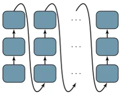
2.2 Deep Transition Architectures

In a deep transition RNN (DT-RNN), at each time step the next state is computed by the sequen-tial application of multiple transition layers, effec-tively using a feed-forward network embedded in-side the recurrent cell. In our experiments, these layers are GRU transition blocks with indepen-dently trainable parameters, connected such that the "state" output of one of them is used as the "state" input of the next one. Note that each of these GRU transition is not individually recurrent, recurrence only occurs at the level of the whole multi-layer cell, as the "state" output of the last

. . . . . . . . .

Figure 1: Deep transition decoder

GRU transition for the current time step is carried over as the "state" input of the first GRU transition for the next time step.

Applying this architecture to NMT is a novel contribution.

2.2.1 Deep Transition Encoder

As in a baseline shallow Nematus system, the en-coder is a bidirectional recurrent neural network. LetLs be the encoder recurrence depth, then for the i-th source word in the forward direction the forward source word state−→hi ≡ −→hi,Ls is

com-puted as: − →

hi,1=GRU1

xi,−→hi−1,Ls

− →_h

i,k =GRUk

0,−→hi,k−1

for1< k_≤Ls

where the input to the first GRU transition is the word embedding xi, while the other GRU transi-tions have no external inputs. Recurrence occurs as the previous word state−→h_i−1,Lsenters the

com-putation in the first GRU transition for the current word.

The reverse source word states are computed sim-ilarly and concatenated to the forward ones to form the bidirectional source word states C _≡

nh_−→

hi,Ls

←− hi,Ls

io

.

2.2.2 Deep Transition Decoder

architecture to an arbitrary transition depthLt as follows:

sj,1=GRU1(yj−1, sj−1,Lt)

sj,2=GRU2(ATT(C, sj,1), sj,1)

sj,k =GRUk(0, sj,k−1)for2< k≤Lt

whereyj−1is the embedding of the previous target

word and ATT(C, si,1)is the context vector

com-puted by the attention mechanism. GRU transi-tions other than the first two do not have external inputs. The target word state vectorsj ≡ sj,Lt is

then used by the feed-forward output network to predict the current target word. A diagram of this architecture is shown in Figure1.

The output network can be also made deeper by adding more feed-forward hidden layers.

2.3 Stacked architectures

A stacked RNN is obtained by having multiple RNNs (GRUs in our experiments) run for the same number of time steps, connected such that at each step the bottom RNN takes "external" inputs from the outside, while each of the higher RNN takes as its "external" input the "state" output of the one below it. Residual connections between states at different depth (He et al., 2016) are also used to improve information flow. Note that unlike deep transition GRUs, here each GRU transition block constitutes a cell that is individually recurrent, as it has its own state that is carried over between time steps.

2.3.1 Stacked Encoder

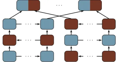
In this work we consider two types of bidirectional stacked encoders: an architecture similar toZhou et al.(2016) which we denote here asalternating

encoder (Figure 2), and one similar to Wu et al. (2016) which we denote as biunidirectional en-coder (Figure3).

Our contribution is the empirical comparison of these architectures, both in isolation and in combi-nation with the deep transition architecture.

We do not consider stacked unidirectional en-coders (Sutskever et al.,2014) as bidirectional en-coders have been shown to outperform them (e.g. Britz et al.(2017)).

Alternating Stacked Encoder The forward part of the encoder consists of a stack of GRU recurrent neural networks, the first one processing words in

. . . .

. . . .

. . . .

. . .

Figure 2: Alternating stacked encoder (Zhou et al., 2016).

the forward direction, the second one in the back-ward direction, and so on, in alternating direc-tions. For an encoder stack depthDs, and a source sentence lengthN, the forward source word state −

→_{wi ≡ −}→_wi,D

s is computed as:

−

→_wi,1=−→_hi,1=GRU1xi,−→_hi −1,1

− →

hi,2k=GRU2k

− →_w

i,2k−1,−→hi+1,2k

for1<2k≤Ds −

→_h

i,2k+1=GRU2k+1

−

→_wi,2k,−→_hi −1,2k+1

for1<2k+ 1_≤Ds −

→_w

i,j =−→hi,j+−→wi,j−1

for1< j≤Ds

where we assume that−→h0,kand−→hN+1,k are zero vectors. Note the residual connections: at each level above the first one, the word state of the pre-vious level−→wi,j−1 is added to the recurrent state

of the GRU cell−→hi,jto compute the the word state for the current level−→wi,j.

The backward part of the encoder has the same structure, except that the first level of the stack processes the words in the backward direction and the subsequent levels alternate directions.

The forward and backward word states are then concatenated to form bidirectional word states C ≡ {[−→wi,Ds←w−i,Ds]}. A diagram of this

archi-tecture is shown in Figure2.

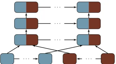
Biunidirectional Stacked Encoder In this en-coder the forward and backward parts are shal-low, as in the baseline architecture. Their word states are concatenated to form shallow bidirec-tional word stateswi ≡ [−→wi,1←w−i,1]that are then

. . . . . . .

. . . . . .

Figure 3: Biunidirectional stacked encoder (Wu et al.,2016).

. . . . . . . . .

Figure 4: Stacked RNN decoder

GRUs have a state size twice that of the base ones. This architecture has shorter maximum in-formation propagation paths than the alternating encoder, suggesting that it may be less expressive, but it has the advantage of enabling implementa-tions with higher model parallelism. A diagram of this architecture is shown in Figure3.

In principle, alternating and biunidirectional stacked encoders can be combined by havingDsa alternating layers followed byDsb unidirectional layers.

2.3.2 Stacked Decoder

A stacked decoder can be obtained by stacking RNNs which operate in the forward sentence di-rection. A diagram of this architecture is shown in Figure4.

Note that the base RNN is always a conditional GRU (cGRU,Firat and Cho,2016) which has tran-sition depth at least two due to the way that the context vectors generated by the attention mecha-nism are used in Nematus. This opens up the pos-sibility of several architectural variants which we evaluated in this work:

Stacked GRU The higher RNNs are simple GRUs which receive as input the state from the previous level of the stack, with residual

connec-tions between the levels.

sj,1,1 =GRU1,1(yj−1, sj−1,1,2)

cj,1 =ATT(C, sj,1,1)

sj,1,2 =GRU1,2(cj,1, sj,1,1)

rj,1 =sj,1,2

sj,k,1 =GRUk(rj,k−1, sj−1,k,1)

rj,k =sj,k,1+rj,k−1

for1< k≤Dt

Note that the higher levels have transition depth one, unlike the base level which has two.

Stacked rGRU The higher RNNs are GRUs whose "external" input is the concatenation of the state below and the context vector from the base RNN. Formally, the states sj,k,1 of the higher

RNNs are computed as:

sj,k,1 =GRUk([rj,k−1, cj,1], sj−1,k,1)

for1< k_≤Dt

This is similar to the deep decoder by Wu et al. (2016).

Stacked cGRU The higher RNNs are condi-tional GRUs, each with an independent attention mechanism. Each level has two GRU transitions per stepj, with a new context vectorcj,kcomputed in between:

sj,k,1 =GRUk,1(rj,k−1, sj−1,k,1)

cj,k =ATT(C, sj,k,1)

sj,k,2 =GRUk,2(cj,k, sj,1,1)

for1< k≤Dt

Note that unlike the stacked GRU and rGRU, the higher levels have transition depth two.

Stacked crGRU The higher RNNs are condi-tional GRUs but they reuse the context vectors from the base RNN. Like the cGRU there are two GRU transition per step, but they reuse the context vectorcj,1 computed at the first level of the stack:

sj,k,1 =GRUk,1(rj,k−1, sj−1,k,1)

sj,k,2 =GRUk,2(cj,1, sj,1,1)

2.4 BiDeep architectures

We introduce the BiDeep RNN, a novel architec-ture obtained by combining deep transitions with stacking.

A BiDeep encoder is obtained by replacing the Dsindividually recurrent GRU cells of a stacked encoder with multi-layer deep transition cells each composed byLsGRU transition blocks.

For instance, the BiDeep alternating encoder is defined as follows:

−

→_wi,1=−→_{hi,1=DTGRU1xi,}−→_hi −1,1

− →

hi,2k=DTGRU2k

− →_w

i,2k−1,−→hi+1,2k

for1<2k≤Ds −

→

hi,2k+1=DTGRU2k+1

− →_w

i,2k,−→hi−1,2k+1

for1<2k+ 1_≤Ds −

→_w

i,j =−→hi,j+−→wi,j−1

for1< j≤Ds

where each multi-layer cell DTGRUk is defined as:

vk,1=GRUk,1(ink,statek)

vk,t=GRUk,t(0, vkt−1)for1< k≤Ls

DTGRUk(ink,statek) =vk,Ls

It is also possible to have different transition depths at each stacking level.

BiDeep decoders are similarly defined, replac-ing the recurrent cells (GRU, rGRU, cGRU or cr-GRU) with deep transition multi-layer cells.

3 Experiments

All experiments were performed with Nematus (Sennrich et al.,2017b), followingSennrich et al. (2017a) in their choice of preprocessing and hy-perparameters. For experiments with deep mod-els, we increase the depth by a factor of 4 com-pared to the baseline for most experiments; in pre-liminary experiments, we observed diminishing returns for deeper models.

We trained on the parallel English–German training data of WMT-2017 news translation task, using newstest2013 as validation set. We used early-stopping on the validation cross-entropy and selected the best model based on validation BLEU.

We report cross-entropy (CE) on newstest2013, training speed (on a single Titan X (Pascal) GPU),

and the number of parameters. For transla-tion quality, we report case-sensitive, detokenized BLEU, measured with mteval-v13a.pl, on

new-stest2014, newstest2015, and newstest2016. We release the code under an open source li-cense, including it in the official Nematus reposi-tory.2 _{The configuration files needed to replicate}

our experiments are available in a separate reposi-tory.3

3.1 Layer Normalization

Our first experiment is concerned with layer nor-malization. We are interested to see how essen-tial layer normalization is for our deep architec-tures, and compare the effect of layer normaliza-tion on a baseline system, and a system with an alternating encoder with stacked depth 4. Results are shown in Table1. We find that layer normal-ization is similarly effective for both the shallow baseline model and the deep encoder, yielding an average improvement of 0.8–1 BLEU, and

reduc-ing trainreduc-ing time substantially. Therefore we use it for all the subsequent experiments.

3.2 Deep Encoders

In Table2we report experimental results for dif-ferent architectures of deep encoders, while the decoder is kept shallow.

We find that all the deep encoders perform sub-stantially better than baseline (+0.5–+1.2 BLEU),

with no consistent quality differences between each other. In terms of number of parameters and training speed, the deep transition encoder per-forms best, followed by the alternating stacked encoder and finally the biunidirectional encoder (note that we trained on a single GPU, the biu-nidirectional encoder may be comparatively faster on multiple GPUs due to its higher model paral-lelism).

3.3 Deep Decoders

Table3shows results for different decoder archi-tectures, while the encoder is shallow. We find that the deep decoders all improve the cross-entropy, but the BLEUresults are more varied: deep output4

decreases BLEUscores (but note that the baseline 2_{https://github.com/EdinburghNLP/}

nematus

3_{https://github.com/Avmb/}

deep-nmt-architectures

encoder CE BLEU parameters (M) training speed early stop

2014 2015 2016 (words/s) (104minibatches)

baseline 49.98 21.2 23.8 28.4 98.0 3350 44

+layer normalization 47.53 21.9 24.7 29.3 98.1 2900 29

alternating (depth 4) 49.25 21.8 24.6 28.9 135.8 2150 46 +layer normalization 46.29 22.6 25.2 30.5 135.9 1600 29

Table 1: Layer normalization results. English→German WMT17 data.

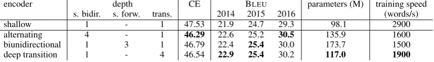
encoder depth CE BLEU parameters (M) training speed

s. bidir. s. forw. trans. 2014 2015 2016 (words/s)

shallow 1 - 1 47.53 21.9 24.7 29.3 98.1 2900

alternating 4 - 1 46.29 22.6 25.2 30.5 135.9 1600

biunidirectional 1 3 1 46.79 22.4 25.4 30.0 173.7 1500

deep transition 1 - 4 46.54 22.9 25.4 30.2 117.0 1900

Table 2: Deep encoder results. English→German WMT17 data. Parameters and speed are highlighted for the deep recurrent models.

has already some depth), stacked GRU performs similarly to the baseline (-0.1–+0.2 BLEU) and

stacked rGRU possibly slightly better (+0.1–+0.2 BLEU).

Other deep RNN decoders achieve higher gains. The best results (+0.6 BLEU on average) are

achieved by the stacked conditional GRU with in-dependent multi-step attention (cGRU). This de-coder, however, is the slowest one and has the most parameters.

The deep transition decoder performs well (+0.5 BLEU on average) in terms of quality and is the

fastest and smallest of all the deep decoders that have shown quality improvements.

The stacked conditional GRU with reused at-tention (crGRU) achieves smaller improvements (+0.3 BLEU on average) and has speed and

size intermediate between the deep transition and stacked cGRU decoders.

3.4 Deep Encoders and Decoders

Table 4shows results for models where both the encoder and the decoder are deep, in addition to the results of the best deep encoder (the deep tran-sition encoder) + shallow decoder reported here for ease of comparison.

Compared to deep transition encoder alone, we generally see improvements in cross-entropy, but not in BLEU. We evaluate architectures similar to Zhou et al.(2016) (alternating encoder + stacked GRU decoder) and (Wu et al., 2016) (biunidirec-tional encoder + stacked rGRU decoder), though they are not straight replications since we used GRU cells rather than LSTMs and the implemen-tation details are different. We find that the for-mer architecture performs better in terms of BLEU

scores, model size and training speed.

The other variants of alternating encoder + stacked or deep transition decoder perform simi-larly to alternating encoder + stacked rGRU de-coder, but do not improve BLEU scores over the

best deep encoder with shallow decoder. Ap-plying the BiDeep architecture while keeping the total depth the same yields small improvements over the best deep encoder (+0.2 BLEU on

aver-age), while the improvement in cross-entropy is stronger. We conjecture that deep decoders may be better at handling subtle target-side linguistic phe-nomena that are not well captured by the 4-gram precision-based BLEUevaluation.

Finally, we evaluate a subset of architectures with a combined depth that is 8 times that of the baseline. Among the large models, the BiDeep model yields substantial improvements (average +0.6 BLEU over the best deep encoder, +1.5

BLEU over the shallow baseline), in addition to

cross-entropy improvements. The stacked-only model, on the other hand, performs similarly to the smaller models, despite having even more param-eters than the BiDeep model. This shows that it is useful to combine deep transitions with stacking, as they provide two orthogonal kinds of depth that are both beneficial for neural machine translation.

3.5 Error Analysis

dis-decoder high RNN decoder RNN depth output CE BLEU params. training speed

stacked trans. type depth 2014 2015 2016 (M) (words/s)

shallow - 1 1 1 47.53 21.9 24.7 29.3 98.1 2900

stacked GRU 4 1 1 46.73 21.8 24.6 29.5 117.0 2250

stacked rGRU 4 1 1 46.72 22.1 25.0 29.4 135.9 2150

stacked cGRU 4 1 1 44.76 22.8 25.5 29.6 164.3 1300

stacked crGRU 4 1 1 45.88 22.5 24.7 29.7 145.4 1750

deep transition - 1 8 1 45.98 22.4 24.9 30.0 117.0 2200

deep output - 1 1 4 47.21 21.5 24.2 28.7 98.9 2850

Table 3: Deep decoder results. English→German WMT17 data. Parameters and speed are highlighted for the deep recurrent models.

encoder decoder decoder high encoder depth decoder depth CE BLEU params. training speed RNN type bidir. forw. trans. stacked trans. 2014 2015 2016 (M) (words/s) shallow shallow - 1 - 1 1 1 47.53 21.9 24.7 29.3 98.1 2900 deep tran. shallow - 1 - 4 1 1 46.54 22.9 25.4 30.2 117.0 1900

(Zhou et al.,2016) (ours)

alternating stacked GRU 4 - 1 4 1 45.89 22.9 25.3 30.1 154.9 1480 (Wu et al.,2016) (ours)

biunidir. stacked rGRU 1 3 1 4 1 46.15 22.4 24.7 29.6 211.5 1280 alternating stacked rGRU 4 - 1 4 1 46.00 23.0 25.7 30.5 173.7 1400 alternating stacked cGRU 4 - 1 4 1 44.32 22.9 25.7 29.8 202.1 970 deep tran. deep tran. - 1 - 4 1 8 45.52 22.7 25.7 30.1 136.0 1570

BiDeep altern. BiDeep rGRU 2 - 2 2 4/2 43.52 23.1 25.5 30.6 145.4 1480 BiDeep altern. BiDeep rGRU 4 - 2 4 4/2 43.26 23.4 26.0 31.0 214.7 980

alternating stacked rGRU 8 - 1 8 1 44.32 22.9 25.5 30.5 274.6 880

Table 4: Deep encoder–decoder results. English→German WMT17 data. Transition depth 4/2 means 4 in the base RNN of the stack and 2 in the higher RNNs. The last two models are large and their results are highlighted separately.

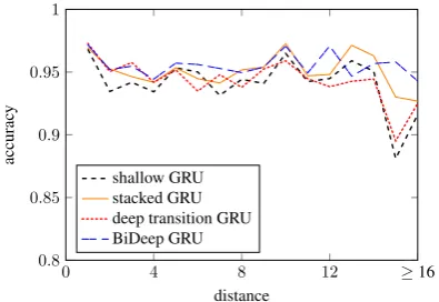
tances, since each layer may lose information dur-ing forward computation or backpropagation. This may not be a significant issue in the encoder, as the attention mechanism provides short paths from any source word state to the decoder, but the decoder contains no such shortcuts between its states, therefore it might be possible that this nega-tively affects its ability to model long-distance re-lationships in the target text, such as subject–verb agreement.

Here, we seek to answer this question by test-ing our models on Ltest-ingeval97 (Sennrich, 2017), a test set which provides contrastive translation pairs for different types of errors. For the exam-ple of subject-verb agreement, contrastive transla-tions are created from a reference translation by changing the grammatical number of the verb, and we can measure how often the NMT model prefers the correct reference over the contrastive variant.

In Figure5, we show accuracy as a function of the distance between subject and verb. We find that information is successfully passed over long distances by the deep recurrent transition network. Even for decisions that require information to be carried over 16 or more words, or at least 128 GRU transitions5_{, the deep recurrent transition network}

5_{some decisions may not require the information to be} passed on the target side because the decisions may be

possi-0 4 8 12 16

0.8 0.85 0.9 0.95 1

distance

accurac

y

shallow GRU stacked GRU deep transition GRU BiDeep GRU

≥16

Figure 5: Subject-verb agreement accuracy as a function of distance between subject and verb.

achieves an accuracy of over 92.5% (N = 560),

higher than the shallow decoder (91.6%), and sim-ilar to the stacked GRU (92.7%). The highest ac-curacy (94.3%) is achieved by the BiDeep net-work.

4 Conclusions

In this work we presented and evaluated multiple architectures to increase the model depth of neural machine translation systems.

stacked encoders (Wu et al., 2016), both in ac-curacy and (single-GPU) speed. We showed that

deep transition architectures, which we first ap-plied to NMT, perform comparably to the stacked ones in terms of accuracy (BLEU, cross-entropy

and long-distance syntactic agreement), and better in terms of speed and number of parameters.

We found that depth improves BLEUscores

es-pecially in the encoder. Decoder depth, however, still improves cross-entropy if not strongly BLEU

scores.

The best results are obtained by our BiDeep architecture which combines both stacked depth and transition depth in both the (alternating) en-coder and the deen-coder, yielding better accuracy for the same number of parameters than systems with only one kind of depth.

We recommend to use combined architectures when maximum accuracy is the goal, or use deep transition architectures when speed or model size are a concern, as deep transition performs very positively in the quality/speed and quality/size trade-off.

While this paper only reports results for one translation direction, the effectiveness of the pre-sented architectures across different data condi-tions and language pairs was confirmed in follow-up work. For the shared news translation task of this year’s Conference on Machine Translation (WMT17), we built deep models for 12 transla-tion directransla-tions, using a deep transitransla-tion architecture or a stacked architecture (alternating encoder and rGRU decoder), and observe improvements for the majority of translation directions (Sennrich et al., 2017a).

Acknowledgments

The research presented in this publication was conducted in cooperation with Samsung Electron-ics Polska sp. z o.o. - Samsung R&D Institute Poland.

This project received funding from the European Union’s Horizon 2020 research and innovation programme under grant agree-ments 645452 (QT21), 644402 (HimL) and 688139 (SUMMA).

References

Lei Jimmy Ba, Ryan Kiros, and Geoffrey E. Hinton. 2016. Layer Normalization.CoRRabs/1607.06450.

Dzmitry Bahdanau, Kyunghyun Cho, and Yoshua Ben-gio. 2015. Neural Machine Translation by Jointly Learning to Align and Translate. InProceedings of the International Conference on Learning Represen-tations (ICLR).

Ondˇrej Bojar, Rajen Chatterjee, Christian Federmann, Yvette Graham, Barry Haddow, Matthias Huck, Antonio Jimeno Yepes, Philipp Koehn, Varvara Logacheva, Christof Monz, Matteo Negri, Aure-lie Neveol, Mariana Neves, Martin Popel, Matt Post, Raphael Rubino, Carolina Scarton, Lucia Spe-cia, Marco Turchi, Karin Verspoor, and Marcos Zampieri. 2016. Findings of the 2016 Conference on Machine Translation (WMT16). InProceedings of the First Conference on Machine Translation, Vol-ume 2: Shared Task Papers. Association for Com-putational Linguistics, Berlin, Germany, pages 131– 198.

Denny Britz, Anna Goldie, Minh-Thang Luong, and Quoc V. Le. 2017. Massive Exploration of Neu-ral Machine Translation Architectures. CoRR

abs/1703.03906.

Mauro Cettolo, Jan Niehues, Sebastian Stüker, Luisa Bentivogli, and Marcello Federico. 2016. Report on the 13th IWSLT Evaluation Campaign. In IWSLT 2016. Seattle, USA.

Kyunghyun Cho, B van Merrienboer, Dzmitry Bah-danau, and Yoshua Bengio. 2014a. On the proper-ties of neural machine translation: Encoder-decoder approaches. InEighth Workshop on Syntax, Seman-tics and Structure in Statistical Translation (SSST-8), 2014.

Kyunghyun Cho, Bart van Merrienboer, Caglar Gul-cehre, Dzmitry Bahdanau, Fethi Bougares, Hol-ger Schwenk, and Yoshua Bengio. 2014b. Learn-ing Phrase Representations usLearn-ing RNN Encoder– Decoder for Statistical Machine Translation. In Pro-ceedings of the 2014 Conference on Empirical Meth-ods in Natural Language Processing (EMNLP). Doha, Qatar, pages 1724–1734.

Orhan Firat and Kyunghyun Cho. 2016.

Con-ditional Gated Recurrent Unit with Attention Mechanism. https://github.com/nyu-dl/dl4mt-tutorial/blob/master/docs/cgru.pdf. Published online, versionadbaeea.

Jonas Gehring, Michael Auli, David Grangier, De-nis Yarats, and Yann N. Dauphin. 2017. Convo-lutional Sequence to Sequence Learning. CoRR

abs/1705.03122.

Razvan Pascanu, Ça˘glar Gülçehre, Kyunghyun Cho, and Yoshua Bengio. 2014. How to Construct Deep Recurrent Neural Networks. InInternational Con-ference on Learning Representations 2014 (Confer-ence Track).

Rico Sennrich. 2017. How Grammatical is Character-level Neural Machine Translation? Assessing MT Quality with Contrastive Translation Pairs. In Pro-ceedings of the 15th Conference of the European Chapter of the Association for Computational Lin-guistics: Volume 2, Short Papers. Association for Computational Linguistics, Valencia, Spain, pages 376–382.

Rico Sennrich, Alexandra Birch, Anna Currey, Ulrich Germann, Barry Haddow, Kenneth Heafield, An-tonio Valerio Miceli Barone, and Philip Williams. 2017a. The University of Edinburgh’s Neural MT Systems for WMT17. In Proceedings of the Sec-ond Conference on Machine Translation, Volume 2: Shared Task Papers. Copenhagen, Denmark.

Rico Sennrich, Orhan Firat, Kyunghyun Cho, Alexan-dra Birch, Barry Haddow, Julian Hitschler, Marcin Junczys-Dowmunt, Samuel Läubli, Antonio Vale-rio Miceli Barone, Jozef Mokry, and Maria Nade-jde. 2017b. Nematus: a Toolkit for Neural Machine Translation. InProceedings of the Software Demon-strations of the 15th Conference of the European Chapter of the Association for Computational Lin-guistics. Association for Computational Linguistics, Valencia, Spain, pages 65–68.

Ilya Sutskever, Oriol Vinyals, and Quoc V Le. 2014. Sequence to sequence learning with neural net-works. InAdvances in neural information process-ing systems. pages 3104–3112.

Ashish Vaswani, Noam Shazeer, Niki Parmar, Jakob Uszkoreit, Llion Jones, Aidan N Gomez, Lukasz Kaiser, and Illia Polosukhin. 2017. Attention Is All You Need. arXiv preprint arXiv:1706.03762.

Yonghui Wu, Mike Schuster, Zhifeng Chen, Quoc V. Le, Mohammad Norouzi, Wolfgang Macherey, Maxim Krikun, Yuan Cao, Qin Gao, Klaus Macherey, Jeff Klingner, Apurva Shah, Melvin Johnson, Xiaobing Liu, Lukasz Kaiser, Stephan Gouws, Yoshikiyo Kato, Taku Kudo, Hideto Kazawa, Keith Stevens, George Kurian, Nishant Patil, Wei Wang, Cliff Young, Jason Smith, Jason Riesa, Alex Rudnick, Oriol Vinyals, Greg Corrado, Macduff Hughes, and Jeffrey Dean. 2016. Google’s Neural Machine Translation System: Bridging the Gap between Human and Machine Translation.

CoRRabs/1609.08144.

Saizheng Zhang, Yuhuai Wu, Tong Che, Zhouhan Lin, Roland Memisevic, Ruslan R Salakhutdinov, and Yoshua Bengio. 2016. Architectural Complexity Measures of Recurrent Neural Networks. In Ad-vances in Neural Information Processing Systems 29. pages 1822–1830.

Jie Zhou, Ying Cao, Xuguang Wang, Peng Li, and Wei Xu. 2016. Deep Recurrent Models with Fast-Forward Connections for Neural Machine Transla-tion. TACL4:371–383.