Section 3: Logistic Regression
As our motivation for logistic regression, we will consider the Challenger disaster, the sex of turtles, college math placement, credit card scoring, and market segmentation.
The Challenger Disaster
On January 28, 1986 the space shuttle, Challenger, had a catastrophic failure due to burn-through of an O-ring seal at a joint in one of the solid-fuel rocket boosters. This was the 25th shuttle flight. Of the 24 previous shuttle flights, 7 had incidents of damage to joints, 16 had no incidents of damage, and 1 was unknown. (The data comes from recovered solid rocket boosters— the one that was unknown was not recovered.) The question we wish to examine is: Could damage to solid-rocket booster field joints be related to cold weather at the time of launch?
Damage to Booster Rocket Field Joints
Below are data from the Presidential Commission on the Space Shuttle Challenger
Accident (1986). The data consist of the flight, temperature at the time of launch (°F) and whether or not there was damage to the booster rocket field joints (No = 0. Yes = 1).
Flight Temp Damage Flight Temp Damage Flight Temp Damage
STS-1 66 NO STS-9 70 NO STS 51-B 75 NO*
STS-2 70 YES STS 41-B 57 YES STS 51-G 70 NO
STS-3 69 NO STS 41-C 63 YES STS 51-F 81 NO
STS-4 80 ??? STS 41-D 70 YES STS 51-I 76 NO
STS-5 68 NO STS 41-G 78 NO STS 51-J 79 NO
STS-6 67 NO STS 51-A 67 NO STS 61-A 75 YES
STS-7 72 NO STS 51-C 53 YES STS 61-B 76 NO
STS-8 73 NO STS 51-D 67 NO STS 61-C 58 YES
The temperature when STS 51-L (Challenger) was launched was 31°F.
Overall, there were 7 incidences of joint damage out of 23 flights: 7 30%
23≈ . When the
temperature was below 65°F, all 4 shuttles had joint damage, 4 100%
4 = , and when the
temperature was above 65°F, only 3 out of 19 had joint damage, 3 16%
19≈ . Is there some
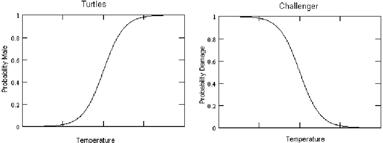
way to predict the chance of booster field joint damage given the temperature at launch? The response variable is the probability of failure (damage)— not necessarily catastrophe. Recall that the temperature was 31°F on the day of the Challenger launch.
Sex of Turtles as it Relates to Incubation Temperature
These data are courtesy of Prof. Ken Koehler, Iowa State University. What determines the sex (male or female) of turtles? Genetics or environment? For a particular species of turtles, temperature seems to have a great effect on sex. Turtle eggs (all one species) were collected from Illinois and put into boxes, with several eggs in each box. These boxes were incubated at different temperatures, with three boxes at each test temperature and temperatures ranging from 27.2°C to 29.9°C. When the eggs hatched, the sex of each turtle was determined.
Temp(°C) Male Female Temp(°C) Male Female Temp(°C) Male Female
27.2 1 9 27.2 0 8 27.2 1 8
27.7 7 3 27.7 4 2 27.7 6 2
28.3 13 0 28.3 6 3 28.3 7 1
28.4 7 3 28.4 5 3 28.4 7 2
29.9 10 1 29.9 8 0 29.9 9 0
Temperature and Gender of Hatched Turtles
The overall proportion of male turtles was 91 0.67
136≈ . When the temperature was below
27.5, the proportion of the turtles that were male was 2 0.07
27= . When the temperature
was below 28, proportion of the turtles that were male was 19 0.37
51≈ . When the
temperature was below 28.5, 64 0.59
108≈ were male, and for temperatures below 30.0, 91
0.67
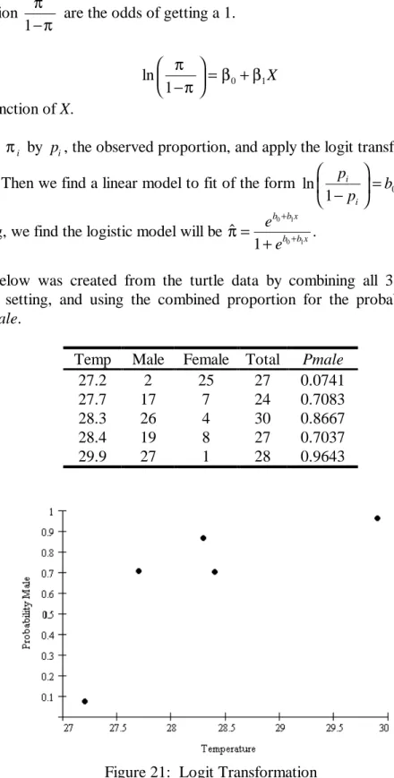
Figure19: Plot of Proportion of Male Turtles vs. Incubation Temperature
Note: We really cannot be sure we have a random sample— we may simply have turtle eggs that were easy to find— not having a random sample might change the error structure.
Is there some way to predict the proportion of male turtles given the incubation temperature? What the scientist wanted to know was at what temperature would there be a 50/50 split in male/female.
Other situations naturally lead to analysis through logistic regression. A few examples are given below:
College Math Placement
Use ACT or SAT scores to predict whether individuals would receive a grade of B or better in an entry level math course and so should be placed in a higher level math course.
Credit Card Scoring
Use various demographic and credit history variables to predict if individuals will be good or bad credit risks.
Market Segmentation
Use various demographic and purchasing information to predict if individuals will purchase from a catalog sent to their homes.
All of these situations involve the idea of prediction, and all have a binary response, for instance, damage/no damage, or male/female. One is interested in predicting a chance, probability, proportion, or percentage. Unlike other prediction situations, the response is bounded with 0≤ ≤p 1.
Logistic Regression
Logistic regression is a statistical technique that can be used in binary response problems. We will need to transform the response to use this technique— what else will we need to change?
We define our binary responses as:
Yi =1→damage to field joint and Yi =0→no damage.
Yi =1→male turtle hatched and Yi =0→female turtle hatched.
Yi =1→receive a B or better and Yi =0→don't receive a B or better.
Yi =1→good credit risk and Yi =0→not good credit risk.
Yi =1→will purchase from catalog and Yi =0→will not purchase from catalog. In each situation, we are interested in predicting the probability that Y =1 from the predictor variable. Here we are only interested in finding a prediction model. Inference is not an issue. The binary form of the response necessarily violates the normality and equal variance assumptions on the errors, so if we were to do inference we would need different methods from those used in ordinary least squares regression.
We denote Prob(Yi = =1) πi and Prob(Yi =0)= −1 πi and E Y( )i =0 1( − πi)+ 1(πi)=πi We want to predict P Y
(
i = =1)
πi from a given x-value, xi. Can we fit this with a linear model of the form E Y X( i i)=β0+ β1Xi =πi ?There are a few problems that distinguish this from more typical regression problems. 1. There is a constraint on the response, which is bounded between 0 and 1, that is,
0≤E Y X( i i)=πi ≤1
2. There is a non-constant variance on the response. We know, since this is a binomial situation, that Var( )εi =Var Y( )i =πi(1− πi). Consequently, the variance depends on the value of Xi.
3. Non-normal error terms: εi = −Yi
(
β0+ β1Xi)
. When Yi =1, we have(
0 1)
1
i Xi
ε = − β + β
When the response variable is binary, or a binomial proportion, the shape of the expected response is often a curve. The S-shaped curve shown below is known as the logistic curve.
Figure 20: Increasing and Decreasing Logistic Plots
Logistic Curvilinear Model
The model used in logistic regression has the form below:
(
)
( (0 1 )) 0 1 | 1 i i X i i i X e E Y X e β β β β π + + = = +The parameters to be estimated show up in the exponent in both numerator and denominator. As before, we will use a transformation to linearize the data, fit a linear model to the transformed data, and re-write to return to the original scale. What transformation will linearize something as complicated as the equation above?
The Logit Transformation
The logit transformation is developed by considering the equation
0 1 0 1 1 X X e e β β β β π = + + + . (We
suppress the subscripts to keep the algebra clean.) If 0 1 0 1 1 X X e e β β β β π = + + + , then 0 1 0 1 0 1 0 1 0 1 1 1 1 1 1 1 X X X X X e e e e e β β β β β β β β β β π + ++ + + + − = − = + + + and 0 1 1 X eβ β π π = + − .
The expression
1 π
π
− are the odds of getting a 1. So, 0 1 ln 1 X π β β π = + − is a linear function of X.
We estimate πi by pi, the observed proportion, and apply the logit transformation,
ln 1 i i p p −
. Then we find a linear model to fit of the form ln 1 0 1
i i p b b x p = + − . By back
transforming, we find the logistic model will be π =$ + + + e e b b x b b x 0 1 0 1 1 .
The table below was created from the turtle data by combining all 3 groups at each temperature setting, and using the combined proportion for the probability of a male, denoted Pmale.
Temp Male Female Total Pmale
27.2 2 25 27 0.0741
27.7 17 7 24 0.7083
28.3 26 4 30 0.8667
28.4 19 8 27 0.7037
29.9 27 1 28 0.9643
Temp Pmale, pi ln 1 i i p p − 27.2 0.0741 -2.5257 27.7 0.7083 0.8873 28.3 0.8667 1.8718 28.4 0.7037 0.8650 29.9 0.9643 3.2958
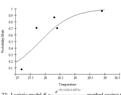
Logit transformation and simple linear regression gives the model to the re-expressed data as
ˆ 51.1116 1.8371X
π′= − + , where πˆ′ represents the fitted values for ln 1 π π −
We now take the predicted values of ln 1
π π −
given by π$′i and back-transform to find the predicted value of π$i. Note that the values of ˆπi are obtained by applying
ˆ ˆ ˆ 1 i i i e e π π π = ′′ + to each π$′i value. Sex of Turtles
Temp Predicted Logit, π$′i Predicted π$i
27.2 -1.1420 0.242
27.7 -0.2234 0.444
28.3 0.8789 0.707
28.4 1.0626 0.743
The graph of the logistic model 51.1122 1.8371 51.1122 1.8371 ˆ 1 x x e e π = − − + +
+ against the data is given below.
Figure 22: Logistic model
51.1122 1.8371 51.1122 1.8371 ˆ 1 x x e e π = − − + +
+ graphed against the data
As we can see, the Logit transformation has adjusted for the curved nature of the response. It has not, however, helped with the problem of violating assumptions on the errors in Simple Linear Regression. Consequently, we can not use standard inference methods with this model.
Maximum Likelihood Approach
To improve the quality of the fit and allow for the use of inference procedures, we can use maximum likelihood techniques rather than the least squares methods. First, define the likelihood function
(
(
0 1)
)
(
)
1 1 , ; i 1 i n Y Y i i i L β β Data π π − = =∏
− , with ( ) ( ) 0 1 0 1 1 i i X i X e e β β β β π = + + + . Notethat when Yi =1, this factor is πi; when Yi =0, this factor is 1− πi. Now, choose β0 and
β1 so as to maximize the likelihood for any given data. For Simple Linear Regression,
minimizing the sum of squared residuals is equivalent to maximizing a normal distribution likelihood.
To find the values of β0 and β1 that maximize the likelihood for this likelihood function given the present data, use the Binary Logistic Regression command in Minitab. You will find it under.
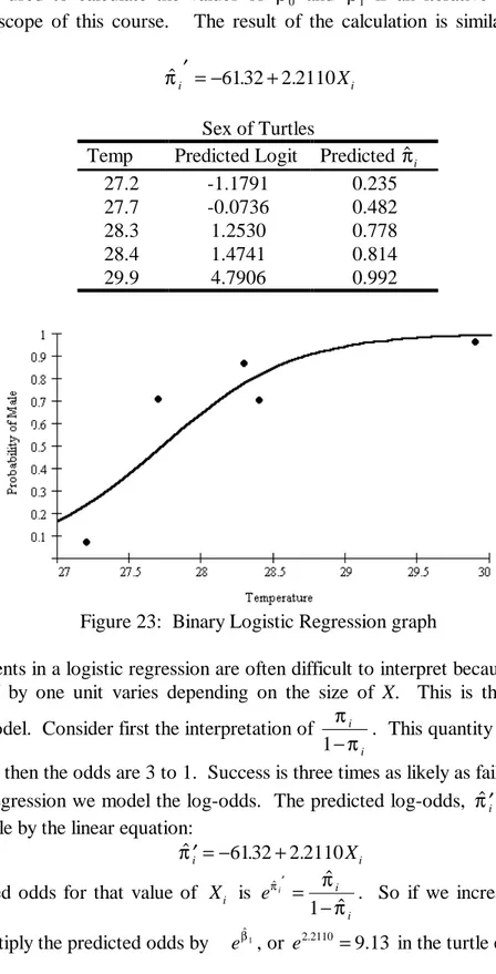
The process used to calculate the values of β0 and β1 is an iterative process that is beyond the scope of this course. The result of the calculation is similar to that from regression:
$ . .
πi′= −61 32 2 2110+ Xi Sex of Turtles
Temp Predicted Logit Predicted π$i
27.2 -1.1791 0.235
27.7 -0.0736 0.482
28.3 1.2530 0.778
28.4 1.4741 0.814
29.9 4.7906 0.992
Figure 23: Binary Logistic Regression graph
The coefficients in a logistic regression are often difficult to interpret because the effect of increasing X by one unit varies depending on the size of X. This is the essence of a
nonlinear model. Consider first the interpretation of π π i
i
1− . This quantity gives the odds. If πi =0 75. , then the odds are 3 to 1. Success is three times as likely as failure.
In logistic regression we model the log-odds. The predicted log-odds, π$′i is given in the turtle example by the linear equation:
π$′= −i 6132 2 2110. + . Xi The predicted odds for that value of Xi is e
i i i $ $ $ π π π ′ = − 1 . So if we increase Xi by one unit, we multiply the predicted odds by eβ$1, or e2.2110 =9.13 in the turtle example. At 27 degrees the predicted odds for a male turtle are approximately 0.20, about 1 to 5. That is, it is 5 times more likely to be a female. At 28 degrees the predicted odds for a
as females. The intercept can be thought of as the log-odds when Xi is zero. The antilog of the intercept may have some meaning as a baseline log-odds, especially if zero is within the range of the original data. Since the temperatures considered run from about 27 to 30 degrees, the value of zero is well outside the range of the data. The intercept, and its antilog, have no practical interpretation in this example.
One of the questions we wanted to answer was, "At what temperature are males and females equally likely?" In this case, the log-odds are equal to 1. So, we can solve the equation
−6132. + 2 211. X =1, so 62.32 28.2 2.211
X = ≈ degrees.
Assessing the Fit
So far we have only looked at estimating parameters and predicting values. The estimates and predictions are subject to variation. We must be able to quantify this variation in order to make inferences. Just as in ordinary regression, we need some means of assessing the fit of a logistic regression model and determining the significance of coefficients in that model.
For logistic regression, the deviance (also known as residual deviance) is used to assess the fit of the overall model. The deviance for a logistic model can be likened to the residual sum of squares in ordinary regression. The smaller the deviance the better the fit of the model. The deviance can be compared to a chi-square distribution, which approximates the distribution of the deviance. This is an asymptotic result that requires large sample sizes. The deviance for the combined turtle data is 14.863 on 3 degrees of freedom. The chance that a χ2 with 3 degrees of freedom exceeds 14.863 is 0.0019. Essentially we are using the deviance to test H0: fit is good versus Ha: fit is not good. The p-value of 0.0019 indicates that the deviance left after the fit is too large to conclude that the fit is good. Thus, there is room for improvement in the model.
Although there is some lack of fit, does temperature give us statistically significant information about the sex of turtles via the logistic regression? Look at the change in deviance when temperature is added to the model. That is, compare deviance when the model is simply ˆπ πi = to the deviance from the logistic model using temperature as the explanatory variable. In Minitab this is summarized by G, the test that all slopes are zero.
49.556
G= on 1 degree of freedom
p-value = 0.000
Alternative Test
The ratio of the estimated coefficient to its standard error, an approximate z-statistic, can
be used to assess significance. In this situation, 2.211 5.13 0.4306
z= = with p=0.000.
Both the z- and the G-statistic indicate that temperature is statistically significant. Since sample sizes are moderate, between 25 and 30, the p-values derived from either test will be approximate, at best. In conclusion, temperature is statistically significant in the logistic regression for the sex of turtles. The logistic regression may not provide the best fit; other models may fit better.
The Challenger Disaster Revisited
Using the techniques of this section, we can fit a linear model to logits from the Challenger data. We will regroup the data by temperature into intervals of 5 degrees, using the midpoint of each interval for the independant variable. We also adjust the probabilities a bit, replacing 0 with 0.01 and 1 with 0.99, so we can take logarithms for the logit fit. Thus, we have the following data: .
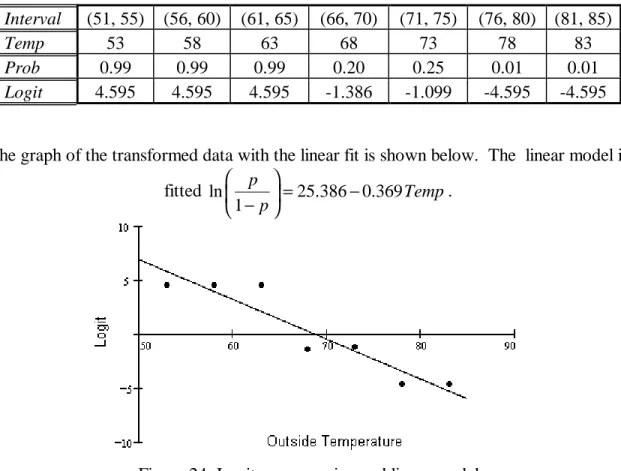
Interval (51, 55) (56, 60) (61, 65) (66, 70) (71, 75) (76, 80) (81, 85)
Temp 53 58 63 68 73 78 83
Prob 0.99 0.99 0.99 0.20 0.25 0.01 0.01
Logit 4.595 4.595 4.595 -1.386 -1.099 -4.595 -4.595
The graph of the transformed data with the linear fit is shown below. The linear model is fitted ln 25.386 0.369 1 p Temp p = − − .
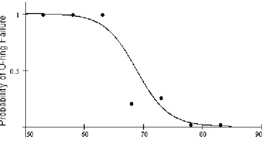
Transforming this model to a probability of failure scale is done by setting 25.386 0.369 25.386 0.369 ˆ 1 Temp Temp e P e − − =
+ . This graph is shown below.
Figure 25: 25.386 0.369 25.386 0.369 1 Temp Temp e P e − − =
+ graphed against the temperauture
From the model we can see that failures will occur at least half of the time if the temperature is below 68.8 degrees. At 31 degrees, the probability is essentially 1 for an O-ring failure.
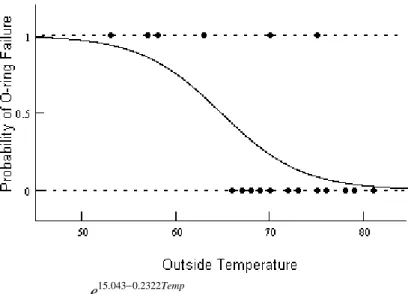
You can also use the ungrouped data with Minitab's Binary Logistic Regression. In that analysis, the Logistic Regression model is
fitted ln 15.043 0.2322 1 p Temp p = − − .
Reversing the logit transformation one has
15.043 0.2322 15.043 0.2322 ˆ 1 Temp Temp e P e − − = + .
From this model, failures will occur at least half of the time if the temperature is below 64.8 degrees.
Figure 26: 15.043 0.2322 15.043 0.2322 1 Temp Temp e P e − − =