CONSIDERING AUTOCORRELATION IN
PREDICTIVE MODELS
Doctoral Dissertation
Jožef Stefan International Postgraduate School Ljubljana, Slovenia, December 2012
Evaluation Board:
Prof. Dr. Marko Bohanec, Chairman, Jožef Stefan Institute, Ljubljana, Slovenia
Assoc. Dr. Janez Demšar, Member, Faculty of Computer and Information Science, University of Ljubljana, Ljubljana, Slovenia Asst. Prof. Michelangelo Ceci, Member, Università degli Studi di Bari “Aldo Moro”, Bari, Italy
MEDNARODNA PODIPLOMSKA ŠOLA JOŽEFA STEFANA
JOŽEF STEFAN INTERNATIONAL POSTGRADUATE SCHOOL
Ljubljana, Slovenia SLOVENIA LJUBLJANA JO ŽE F ST E FA N I NTER NATIONAL POSTG RA D U A T E SC HO OL 2004Daniela Stojanova
CONSIDERING AUTOCORRELATION
IN PREDICTIVE MODELS
Doctoral Dissertation
UPOŠTEVANJE AVTOKORELACIJE V
NAPOVEDNIH MODELIH
Doktorska disertacija
Supervisor:Prof. Dr. Sašo Džeroski
Contents
Abstract xi Povzetek xiii Abbreviations xv Abbreviations xv 1 Introduction 1 1.1 Outline . . . 1 1.2 Motivation . . . 3 1.3 Contributions . . . 51.4 Organization of the dissertation . . . 6
2 Definition of the Problem 9 2.1 Learning Predictive Models from Examples . . . 9
2.1.1 Classification . . . 10
2.1.2 Regression . . . 11
2.1.3 Multi-Target Classification and Regression . . . 12
2.1.4 Hierarchial Multi-Label Classification . . . 13
2.2 Relations Between Examples . . . 14
2.2.1 Types of Relations . . . 15
2.2.2 The Origin of Relations . . . 16
2.2.3 The Use of Relations . . . 19
2.3 Autocorrelation . . . 21
2.3.1 Type of Targets in Predictive Modeling . . . 21
2.3.2 Type of Relations . . . 22
2.4 Summary . . . 32
3 Existing Autocorrelation Measures 33 3.1 Measures of Temporal Autocorrelation . . . 33
3.1.1 Measures for Regression . . . 33
3.1.2 Measures for Classification . . . 35
3.2 Measures of Spatial Autocorrelation . . . 35
3.2.1 Measures for Regression . . . 35
3.2.2 Measures for Classification . . . 41
3.3 Measures of Spatio-Temporal Autocorrelation . . . 46
3.3.2 Measures for Classification . . . 48
3.4 Measures of Network Autocorrelation . . . 48
3.4.1 Measures for Regression . . . 48
3.4.2 Measures for Classification . . . 49
4 Predictive Modeling Methods that use Autocorrelation 53 4.1 Predictive Methods that use Temporal Autocorrelation . . . 53
4.1.1 Classification Methods . . . 53
4.1.2 Regression Methods . . . 54
4.2 Predictive Methods that use Spatial Autocorrelation . . . 55
4.2.1 Classification Methods . . . 55
4.2.2 Regression Methods . . . 57
4.3 Predictive Methods that use Spatio-Temporal Autocorrelation . . . 60
4.3.1 Classification Methods . . . 60
4.3.2 Regression Methods . . . 61
4.4 Predictive Methods that use Network Autocorrelation . . . 63
4.4.1 Classification Methods . . . 63
4.4.2 Regression Methods . . . 64
5 Learning Predictive Clustering Trees (PCTs) 67 5.1 The Algorithm for Building Predictive Clustering Trees (PCTs) . . . 67
5.2 PCTs for Single and Multiple Targets . . . 68
5.3 PCTs for Hierarchical Multi-Label Classification . . . 71
6 Learning PCTs for Spatially Autocorrelated Data 75 6.1 Motivation . . . 75
6.2 Learning PCTs by taking Spatial Autocorrelation into Account . . . 76
6.2.1 The Algorithm . . . 76
6.2.2 Exploiting the Properties of Autocorrelation in SCLUS . . . 79
6.2.3 Choosing the Bandwidth . . . 80
6.2.4 Time Complexity . . . 80
6.3 Empirical Evaluation . . . 81
6.3.1 Datasets . . . 82
6.3.2 Experimental Setup . . . 83
6.3.3 Results and Discussion . . . 84
6.4 Summary . . . 100
7 Learning PCTs for Network Autocorrelated Data 101 7.1 Motivation . . . 101
7.2 Learning PCTs by taking Network Autocorrelation into Account . . . 102
7.2.1 The Algorithm . . . 102
7.2.2 Exploiting the Properties of Autocorrelation in NCLUS . . . 104
7.2.3 Choosing the Bandwidth . . . 106
7.2.4 Time Complexity . . . 106
7.3 Empirical Evaluation . . . 107
7.3.1 Datasets . . . 107
7.3.2 Experimental setup . . . 110
7.3.3 Results and Discussion . . . 111
8 Learning PCTs for HMC from Network Data 119
8.1 Motivation . . . 119
8.2 Measures of autocorrelation in a HMC setting . . . 121
8.2.1 Network Autocorrelation for HMC . . . 121
8.2.2 Global Moran’sI . . . 122
8.2.3 Global Geary’sC . . . 123
8.3 Learning PCTs for HMC by Taking Network Autocorrelation into Account . . . 124
8.3.1 The network setting for NHMC . . . 124
8.3.2 Trees for Network HMC . . . 125
8.4 Empirical Evaluation . . . 129
8.4.1 Data Sources . . . 129
8.4.2 Experimental Setup . . . 130
8.4.3 Comparison between CLUS-HMC and NHMC . . . 130
8.4.4 Comparison with Other Methods . . . 131
8.4.5 Comparison of Different PPI Networks in the Context of Gene Function Predic-tion by NHMC . . . 131
8.5 Summary . . . 133
9 Conclusions and Further Work 137 9.1 Contribution to science . . . 137 9.2 Further Work . . . 139 10 Acknowledgments 141 11 References 143 List of Figures 152 List of Tables 153 List of Algorithms 155
Appendix A: CLUS user manual 160
Appendix B: Bibliography 167
To my family Na mojata familija
Abstract
Most machine learning, data mining and statistical methods rely on the assumption that the analyzed data are independent and identically distributed (i.i.d.). More specifically, the individual examples included in the training data are assumed to be drawn independently from each other from the same probability distribution. However, cases where this assumption is violated can be easily found: For example, species are distributed non-randomly across a wide range of spatial scales. The i.i.d. assumption is often violated because of the phenomenon of autocorrelation.
The cross-correlation of an attribute with itself is typically referred to as autocorrelation: This is the most general definition found in the literature. Specifically, in statistics, temporal autocorrelation is defined as the cross-correlation between the attribute of a process at different points in time. In time-series analysis, temporal autocorrelation is defined as the correlation among time-stamped values due to their relative proximity in time. In spatial analysis, spatial autocorrelation has been defined as the correlation among data values, which is strictly due to the relative location proximity of the objects that the data refer to. It is justified by Tobler’s first law of geography according to which “everything is related to everything else, but near things are more related than distant things”. In network studies, autocorrelation is defined by the homophily principle as the tendency of nodes with similar values to be linked with each other.
In this dissertation, we first give a clear and general definition of the autocorrelation phenomenon, which includes spatial and network autocorrelation for continuous and discrete responses. We then present a broad overview of the existing autocorrelation measures for the different types of autocorrela-tion and data analysis methods that consider them. Focusing on spatial and network autocorrelaautocorrela-tion, we propose three algorithms that handle non-stationary autocorrelation within the framework of predictive clustering, which deals with the tasks of classification, regression and structured output prediction. These algorithms and their empirical evaluation are the major contributions of this thesis.
We first propose a data mining method called SCLUS that explicitly considers spatial autocorrelation when learning predictive clustering models. The method is based on the concept of predictive clustering trees (PCTs), according to which hierarchies of clusters of similar data are identified and a predictive model is associated to each cluster. In particular, our approach is able to learn predictive models for both a continuous response (regression task) and a discrete response (classification task). It properly deals with autocorrelation in data and provides a multi-level insight into the spatial autocorrelation phenomenon. The predictive models adapt to the local properties of the data, providing at the same time spatially smoothed predictions. We evaluate our approach on several real world problems of spatial regression and spatial classification.
The problem of “network inference” is known to be a challenging task. In this dissertation, we propose a data mining method called NCLUS that explicitly considers autocorrelation when building predictive models from network data. The algorithm is based on the concept of PCTs that can be used for clustering, prediction and multi-target prediction, including multi-target regression and multi-target classification. We evaluate our approach on several real world problems of network regression, coming from the areas of social and spatial networks. Empirical results show that our algorithm performs better
than PCTs learned by completely disregarding network information, CLUS* which is tailored for spatial data, but does not take autocorrelation into account, and a variety of other existing approaches.
We also propose a data mining method called NHMC for (Network) Hierarchical Multi-label Classi-fication. This has been motivated by the recent development of several machine learning algorithms for gene function prediction that work under the assumption that instances may belong to multiple classes and that classes are organized into a hierarchy. Besides relationships among classes, it is also possible to identify relationships among examples. Although such relationships have been identified and exten-sively studied in the literature, in particular as defined by protein-to-protein interaction (PPI) networks, they have not received much attention in hierarchical and multi-class gene function prediction. Their use introduces the autocorrelation phenomenon and violates the i.i.d. assumption adopted by most ma-chine learning algorithms. Besides improving the predictive capabilities of learned models, NHMC is helpful in obtaining predictions consistent with the network structure and consistently combining two information sources (hierarchical collections of functional class definitions and PPI networks). We com-pare different PPI networks (DIP, VM and MIPS for yeast data) and their influence on the predictive capability of the models. Empirical evidence shows that explicitly taking network autocorrelation into account can increase the predictive capability of the models, especially when the PPI networks are dense. NHMC outperforms CLUS-HMC (that disregards the network) for GO annotations, since these are more coherent with the PPI networks.
Povzetek
Veˇcina metod za podatkovno rudarjenje, strojno uˇcenje in statistiˇcno analizo podatkov temelji na pred-postavki, da so podatki neodvisni in enako porazdeljeni (ang. independent and identically distributed – i.i.d.). To pomeni, da morajo biti uˇcni primeri med seboj neodvisni ter imeti enako verjetnostno po-razdelitev. Vendar so primeri, ko podatki niso i.i.d., v praksi zelo pogosti. Tako so na primer živalske vrste porazdeljene po prostoru nenakljuˇcno. Predpostavka i.i.d. je pogosto kršena zaradi avtokorelacije.
Najbolj splošna definicija avtokorelacije je, da je to preˇcna korelacija atributa samega s seboj. V statistiki je ˇcasovna avtokorelacija definirana kot preˇcna korelacija med atributom procesa ob razliˇcnem ˇcasu. Pri analizi ˇcasovnih vrst je ˇcasovna avtokorelacija definirana kot korelacija med ˇcasovno odvisnimi vrednostmi zaradi njihove relativne ˇcasovne bližine. V prostorski analizi je prostorska avtokorelacija definirana kot korelacija med podatkovnimi vrednostmi, ki je nastala samo zaradi relativne bližine ob-jektov, na katero se nanašajo podatki. Definicija temelji na prvem Toblerjevem zakonu o geografiji, po katerem “je vse povezano z vsem, vendar so bližje stvari bolj povezane kot oddaljene stvari.” Pri analizi omrežij je avtokorelacija definirana s pomoˇcjo naˇcela homofilnosti, ki pravi, da vozlišˇca s podobnimi vrednostmi težijo k medsebojni povezanosti.
V disertaciji najprej podamo jasno in splošno definicijo avtokorelacije, ki vkljuˇcuje prostorsko in omrežno avtokorelacijo za zvezne in diskretne spremenljivke. Nato predstavimo obširen pregled obsto-jeˇcih mer za avtokorelacijo skupaj z metodami za analizo podatkov, ki jih uporabljajo. Osredotoˇcimo se na prostorsko in omrežno avtokorelacijo in predlagamo tri algoritme, ki upoštevajo spremenljivo avtoko-relacijo v okviru napovednega razvršˇcanja. Na ta naˇcin lahko obravnavamo klasifikacijske in regresijske naloge ter napovedovanje strukturiranih spremenljivk. Ti trije algoritmi in njihovo empiriˇcno vrednotenje so glavni prispevek disertacije.
Najprej predlagamo metodo podatkovnega rudarjenja SCLUS, ki izrecno upošteva prostorsko av-tokorelacijo pri uˇcenju modelov za napovedno razvršˇcanje. Metoda temelji na gradnji odloˇcitvenih dreves za napovedno razvršˇcanje (DNR), pri kateri podatke razvrstimo v hierarhiˇcno strukturo s skupinami med seboj podobnih podatkov ter vsaki skupini predružimo napovedni model. Naša metoda omogoˇca uˇcenje napovednih modelov za zvezne in diskretne ciljne spremenljivke (klasifikacija in re-gresija). Metoda pravilno upošteva avtokorelacijo v podatkih in omogoˇca veˇcnivojski vpogled v pojav prostorske avtokorelacije. Napovedni modeli se prilagajajo lokalnim lastnostim podatkov in hkrati zago-tavljajo gladko spreminjanje napovedi v prostoru. Naš pristop ovrednotimo na veˇc razliˇcnih realnih problemih prostorske regresije in klasifikacije.
Problem “omrežnega sklepanja” je znan kot zahtevna naloga. V disertaciji predlagamo algoritem podatkovnega rudarjenja z imenom NCLUS, ki izrecno upošteva avtokorelacijo pri gradnji napovednih modelov na podatkih o omrežjih. Algoritem temelji na konceptu dreves za napovedno razvršˇcanje, ki jih je mogoˇce uporabiti za razvršˇcanje, regresijo in klasifikacijo preprostih ali strukturiranih spremenljivk. Naš pristop ovrednotimo na veˇc razliˇcnih realnih problemih s podroˇcja socialnih in prostorskih omrežij. Empiriˇcni rezultati kažejo, da naš algoritem deluje bolje kot navadna drevesa za napovedno razvršˇcanje, zgrajena brez upoštevanja informacij o omrežjih, bolje kot metoda CLUS*, ki je prilagojena za analizo prostorskih podatkov, a ne upošteva avtokorelacije, in bolje od drugih obstojeˇcih pristopov.
Predlagamo tudi metodo podatkovnega rudarjenja NHMC za hierarhiˇcno veˇcznaˇckovno klasifikacijo. Motivacija za ta pristop je bil nedavni razvoj razliˇcnih algoritmov strojnega uˇcenja za napovedovanje funkcij genov, ki delujejo pod predpostavko, da lahko primeri sodijo v veˇc razredov, ti razredi pa so organizirani v hierarhijo. Poleg odvisnosti med razredi, je mogoˇce doloˇciti tudi odvisnosti med primeri.
ˇ
Ceprav so te povezave identificirane in obširno raziskane v literaturi, še posebej v primeru omrežij in-terakcij med proteini (IMP), pa še vedno niso dovolj upoštevane v okviru hierarhiˇcne veˇcznaˇckovne klasifikacije funkcij genov. Njihova uporaba uvaja avtokorelacijo in krši predpostavko neodvisnosti med primeri, na kateri temelji veˇcina algoritmov strojnega uˇcenja. Poleg izboljšane napovedne toˇcnosti nauˇcenih modelov, nam NHMC omogoˇca napovedi, ki so skladne s strukturo omrežja in konsistentno up-oštevajo dva razliˇcna vira informacij (hierarhiˇcne zbirke funkcijskih razredov in omrežij IMP). Primerjali smo tri razliˇcna omrežja IMP (DIP, VM in MIPS pri kvasovkah) in njihovo napovedno toˇcnost. Empiriˇcni rezultati kažejo, da upoštevanje omrežne avtokorelacije izboljša napovedno toˇcnost modelov, še posebej v primeru, ko so omrežja IMP gosta. Metoda NHMC dosega boljše rezultate kot metoda CLUS-HMC (ki ne upošteva omrežja) za oznake GO (Gene Ontology), ker so te bolj usklajene z omrežji IMP.
Abbreviations
AUPRC = Area Under the Precision-Recall Curve
AU PRC = Average AUPRC
AUPRC = Area Under the average Precision-Recall Curve
ARIMA = AutoRegressive Integrated Moving Average
ARMA = AutoRegressive Moving Average
AR = AutoRegressive Model
CAR = Conditional AutoRegressive Model
CCF = Cross-Correlation Function
CC = Correlation Coefficient
CLUS = Software for Predictive Clustering, learns PCTs CLUS-HMC = CLUS for Hierarchical Multi-label Classification
DAG = Directed Acyclic Graph
DM = Data Mining
GIS = Geographic Information System
GO = Gene Ontology
GWR = Geographically Weighted Regression
HMC = Hierarchical Multi-label Classification
ILP = Inductive Logic Programming
ITL = Iterative Transductive Regression
LiDAR = Light Detection and Ranging
MA = Moving Average Model
ML = Machine Learning
MRDM = Multi-Relational Data Mining
MTCT = Multi-Target Classification Tree
MTDT = Multi-Target Decision Tree
MT = Model Trees
NCLUS = Network CLUS
NHMC = Network CLUS for Hierarchical Multi-label Classification
PCT = Predictive Clustering Tree
PPI = Protein to Protein Interaction
PR = Precision-Recall
RMSE = Root Mean Squared Error
RRMSE = Relative Root Mean Squared Error
RS = Remote Sensing
RT = Regression Trees
SAR = Spatial AutoRegressive Model
SCLUS = Spatial CLUS
SPOT = Système Pour L’observation de la Terre
STARIMA = Spatio-Temporal AutoRegressive Integrated Moving Average
1
1
Introduction
In this introductory chapter, we first place the dissertation within the broader context of its research area. We then motivate the research performed within the scope of the dissertation. The major contributions of the thesis to science are described next. We conclude this chapter by giving an outline of the structure of the remainder of the thesis.
1.1
Outline
The research presented in this dissertation is placed in the area of artificial intelligence (Russell and Norvig, 2003), and more specifically in the area of machine learning. Machine learning is concerned with the design and the development of algorithms that allow computers to evolve behaviors based on empirical data, i.e., it studies computer programs that automatically improve with experience (Mitchell, 1997). A major focus of machine learning research is to extract information from data automatically by computational and statistical methods and make intelligent decisions based on the data. However, the difficulty lies in the fact that the set of all possible behaviors, given all possible inputs, is too large to be covered by the set of observed examples.
In general, there are two types of learning: inductive and deductive. Inductive machine learning (Bratko, 2000) is a very significant field of research in machine learning, where new knowledge is ex-tracted out of data that describes experience and is given in the form of learning examples (instances). In contrast, deductive learning (Langley, 1996) explains a given set of rules by using specific information from the data.
Depending on the feedback the learner gets during the learning process, learning can be classified as supervised or unsupervised. Supervised learning is a machine learning technique for learning a function from a set of data. Supervised inductive machine learning, also called predictive modeling, assumes that each learning example includes some target property, and the goal is to learn a model that accu-rately predicts this property. On the other hand, unsupervised inductive machine learning, also called descriptive modeling, assumes no such target property to be predicted. Examples of machine learning methods for predictive modeling include decision trees, decision rules and support vector machines. In contrast, examples of machine learning methods for descriptive modeling include clustering, association rule modeling and principal-component analysis (Bishop, 2007).
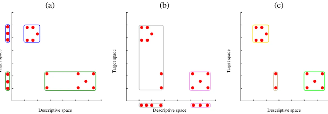
In general, predictive and descriptive modeling are considered as different machine learning tasks and are usually treated separately. However, predictive modeling can be seen as a special case of clustering (Blockeel, 1998). In this case, the goal of predictive modeling is to identify clusters that are compact in the target space (i.e., group the instances with similar values of the target variable). The goal of descriptive modeling, on the other hand, is to identify clusters compact in the descriptive space (i.e., group the instances with similar values of the descriptive variables).
Predictive modeling methods are used for predicting an output (i.e., target property or target attribute) for an example. Typically, the output can be either a discrete variable (classification) or a continuous variable (regression). However, there are many real-life problems, such as text categorization, gene function prediction, image annotation, etc., where the input and/or the output are structured. Beside the
2 Introduction
typical classification and regression task, we also consider the latter, namely, predictive modeling tasks with structured outputs.
Predictive clustering (Blockeel, 1998) combines elements from both prediction and clustering. As in clustering, clusters of examples that are similar to each other are identified, but a predictive model is associated to each cluster. New instances are assigned to clusters based on cluster descriptions. The associated predictive models provide predictions for the target property. The benefit of using predictive clustering methods, as in conceptual clustering (Michalski and Stepp, 2003), is that besides the clusters themselves, they also provide symbolic descriptions of the constructed clusters. However, in contrast to conceptual clustering, predictive clustering is a form of supervised learning.
Predictive clustering trees (PCTs) are tree structured models that generalize decision trees. Key properties of PCTs are that i)they can be used to predict many or all attributes of an example at once (multi-target),ii)they can be applied to a wide range of prediction tasks (classification and regression) andiii)they can work with examples represented by means of a complex representation (Džeroski et al, 2007), which is achieved by plugging in a suitable distance metric for the task at hand. PCTs were first implemented in the context of First-Order logical decision trees, in the system TILDE (Blockeel, 1998), where relational descriptions of the examples are used. The most known implementation of PCTs, however, is the one that uses attribute-value descriptions of the examples and is implemented in the predictive clustering framework of the CLUS system (Blockeel and Struyf, 2002). The CLUS system is available for download athttp://sourceforge.net/projects/clus/.
Here, we extend the predictive clustering framework to work in the context of autocorrelated data. For such data the independence assumption which typically underlies machine learning methods and multivariate statistics, is no longer valid. Namely, the autocorrelation phenomenon directly violates the assumption that the data instances are drawn independent from each other from an identical distribution (i.i.d.). At the same time, it offers the unique opportunity to improve the performance of predictive models which would take it into account.
Autocorrelation is very common in nature and has been investigated in different fields, from statistics and time-series analysis, to signal-processing and music recordings. Here we acknowledge the existence of four different types of autocorrelation: spatial, temporal, spatio-temporal and network (relational) autocorrelation, describing the existing autocorrelation measures and the data analysis methods that con-sider them. However, in the development of the proposed algorithms, we focus on spatial autocorrelation and network autocorrelation. In addition, we also deal with the complex case of predicting structured targets (outputs), where network autocorrelation is considered.
In the PCT framework (Blockeel, 1998), a tree is viewed as a hierarchy of clusters: the top-node contains all the data, which is recursively partitioned into smaller clusters while moving down the tree. This structure allows us to estimate and exploit the effect of autocorrelation in different ways at different nodes of the tree. In this way, we are able to deal with non-stationarity autocorrelation, i.e., autocorrela-tion which may change its effects over space/networks structure.
PCTs are learned by extending the heuristics functions used in tree induction to include the spa-tial/network autocorrelation. In this way, we obtain predictive models that are able to deal with au-tocorrelated data. More specifically, beside maximizing the variance reduction which minimizes the intra-cluster distance in the class labels associated to examples, we also maximize cluster homogeneity in terms of autocorrelation at the same time doing the evaluation of candidate splits for adding a new node to the tree. This results in improved predictive performance of the obtained models and in smother predictions.
A diverse set of methods that deal with this kind of data, in several fields of research, already exists in the literature. However, most of them either deal with specific case studies or assume a specific experimental setting. In the next section, we describe the existing methods and motivate our work.
Introduction 3
1.2
Motivation
The assumption that data examples are independent from each other and are drawn from the same prob-ability distribution, i.e., that the examples are independent and identically distributed (i.i.d.), is common to most of the statistical and machine learning methods. This assumption is important in the classical form of the central limit theorem, which states that the probability distribution of the sum (or average) of i.i.d. variables with finite variance approaches a normal distribution. While this assumption tends to simplify the underlying mathematics of many statistical and machine learning methods, it may not be realistic in practical applications of these methods.
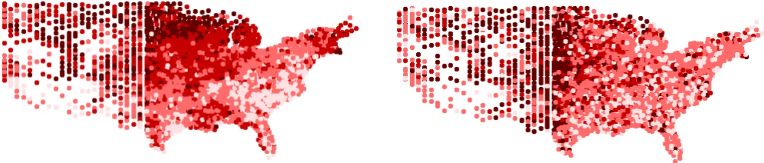
In many real-world problems, data are characterized by a form of autocorrelation, where the value of a variable for a given example depends on the values of the same variable in related examples. This is the case for the spatial proximity relation encounter in spatial data, where data measured at nearby locations often (but not always) influence each other. For example, species richness at a given site is likely to be similar to that of a site nearby, but very much different from sites far away. This is due to the fact that the environment is more similar within a shorter distance and the above phenomenon is referred to as spatial autocorrelation (Tobler, 1970).
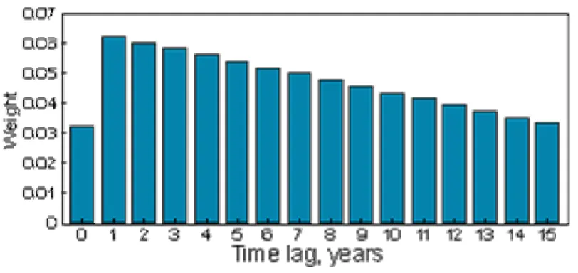
The case of the temporal proximity relation encounter in time-series data is similar: data measured at a given time point are not completely independent of the past values. This phenomenon is referred to as temporal autocorrelation (Epperson, 2000). For example, weather conditions are highly autocorrelated within one year due to seasonality. A weaker correlation exists between weather variables in consecutive years.
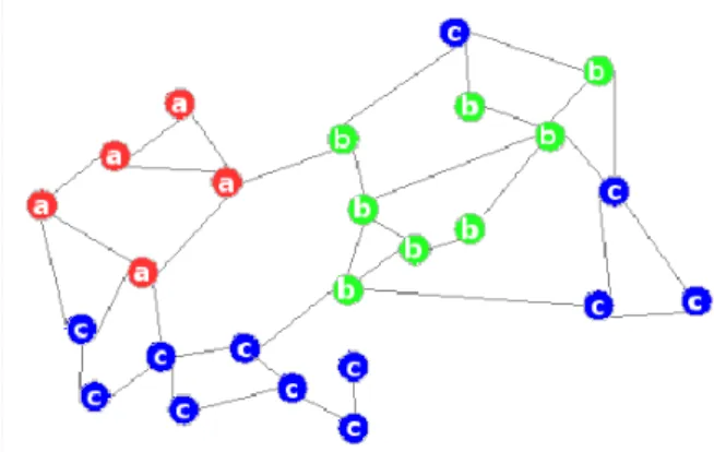
A similar phenomenon also occurs in network data, where the values of a variable at a certain node often (but not always) depend on the values of the variables at the nodes connected to the given node: This phenomenon is referred to as network homophily (Neville et al, 2004). Recently, networks have become ubiquitous in several social, economical and scientific fields ranging from the Internet to social sciences, biology, epidemiology, geography, finance, and many others. Researchers in these fields have demonstrated that systems of different nature can be represented as networks (Newman and Watts, 2006). For instance, the Web can be considered as a network of web-pages, connected with each other by edges representing various explicit relations, such as hyperlinks. Social networks can be seen as groups of members that can be connected by friendship relations or can follow other members because they are interested in similar topics of interests. Gene networks can provide insight about genes and their possible relations of co-regulation based on the similarities of their expression levels. Finally, in epidemiology, networks can represent the spread of diseases and infections.
Moreover, in many real-life problems of predictive modeling, not only the data are not independent and identically distributed (i.i.d.), but the output (i.e., the target property) is structured, meaning that there can be dependencies between classes (e.g., classes are organized into a tree-shaped hierarchy or a directed acyclic graph). These types of problems occur in domains such as the life sciences (predicting gene function), ecology (analysis of remotely sensed data, habitat modeling), multimedia (annotation and retrieval of images and videos), and the semantic web (categorization and analysis of text and web content). The amount of data in these areas is increasing rapidly.
A variety of methods, specialized in predicting a given type of structured output (e.g., a hierarchy of classes (Silla and Freitas, 2011)), have been proposed (Bakır et al, 2007). However, many of them are computationally demanding and not suited for dealing with large datasets and especially with large outputs spaces. The predictive clustering framework offers a unifying approach for dealing with differ-ent types of structured outputs and the algorithms developed in this framework construct the predictive models very efficiently. Moreover, PCTs can be easily interpreted by a domain expert, thus supporting the process of knowledge extraction.
4 Introduction
analysis of such data needs to take this into account.
Such work either removes the autocorrelation dependencies during pre-processing and then use tra-ditional algorithms (e.g., (Hardisty and Klippel, 2010; Huang et al, 2004)) or modifies the classical machine learning, data mining and statistical methods in order to consider the autocorrelation (e.g., (Bel et al, 2009; Rinzivillo and Turini, 2004, 2007)). There are also approaches which use a relational setting (e.g., (Ceci and Appice, 2006; Malerba et al, 2005)), where the autocorrelation is usually incorporated through the data structure or defined implicitly through relationships among the data and other data properties.
However, one limitation of most of the approaches that take autocorrelation into account is that they assume that autocorrelation dependencies are constant (i.e., do not change) throughout the space/network (Angin and Neville, 2008). This means that possible significant variability in autocorrelation dependen-cies in different points of the space/network cannot be represented and modeled. Such variability could result from a different underlying latent structure of the space/network that varies among its parts in terms of properties of nodes or associations between them. For example, different research communities may have different levels of cohesiveness and thus cite papers on other topics with varying degrees. As pointed out by Angin and Neville (2008), when autocorrelation varies significantly throughout a network, it may be more accurate to model the dependencies locally rather than globally.
In the dissertation, we extend the predictive clustering framework in the context of PCTs that are able to deal with data (spatial and network) that do not follow the i.i.d. assumption. The distinctive char-acteristic of the proposed approach is that it explicitly considers the non-stationary (spatial and network) autocorrelation when building the predictive models. Such a method not only extends the applicability of the predictive clustering approach, but also exploits the autocorrelation phenomenon and uses it to make better predictions and better models.
In traditional PCTs (Blockeel, 1998), the tree construction is performed by maximizing variance reduction. This heuristic guarantees, in principle, accurate models since it reduces the error on the training set. However, it neglects the possible presence of autocorrelation in the training data. To address this issue, we propose to simultaneously maximize autocorrelation for spatial/network domains. In this way, we exploit the spatial/network structure of the data in the PCT induction phase and obtain predictive models that naturally deal with the phenomenon of autocorrelation.
The consideration of autocorrelation in clustering has already been investigated in the literature, both for spatial clustering (Glotsos et al, 2004) and network clustering (Jahani and Bagherpour, 2011). Motivated by the demonstrated benefits of considering autocorrelation, we exploit some characteristics of autocorrelated data to improve the quality of PCTs. The consideration of autocorrelation in clustering offers several advantages, since it allows us to:
• determine the strength of the spatial/network arrangement on the variables in the model; • evaluate stationarity and heterogeneity of the autocorrelation phenomenon across space;
• identify the possible role of the spatial/network arrangement/distance decay on the predictions associated with each of the nodes of the tree;
• focus on the spatial/network “neighborhood” to better understand the effects that it can have on other neighborhoods and vice versa.
These advantages of considering spatial autocorrelation in clustering, identified by (Arthur, 2008), fit well into the case of PCTs. Moreover, as recognized by (Griffith, 2003), autocorrelation implicitly defines a zoning of a (spatial) phenomenon: Taking this into account reduces the effect of autocorrelation on prediction errors. Therefore, we propose to perform clustering by maximizing both variance reduction
Introduction 5
and cluster homogeneity (in terms of autocorrelation) at the same time, during the phase of adding a new node to the predictive clustering tree.
The network (spatial and relational) setting that we address in this work is based on the use of both the descriptive information (attributes) and the network structure during training, whereas we only use the descriptive information in the testing phase and disregard the network structure. More specifically, in the training phase, we assume that all examples are labeled and that the given network is complete. In the testing phase, all testing examples are unlabeled and the network is not given. A key property of our approach is that the existence of the network is not obligatory in the testing phase, where we only need the descriptive information. This can be very beneficial when predictions need to be made for those examples for which connections to others examples are not known or need to be confirmed. The more common setting where a network with some nodes labeled and some nodes unlabeled is given, can be easily mapped to our setting. We can use the nodes with labels and the projection of the network on these nodes for training and only the unlabeled nodes without network information in the testing phase.
This network setting is very different from the existing approaches to network classification and regression where the descriptive information is typically in a tight connection to the network structure. The connections (edges in the network) between the data in the training/testing set are predefined for a particular instance and are used to generate the descriptive information associated to the nodes of the network (see, for example, (Steinhaeuser et al, 2011)). Therefore, in order to predict the value of the response variable(s), besides the descriptive information, one needs the connections (edges in the network) to related/similar entities. This is very different from what is typically done in network analysis as well. Indeed, the general focus there is on exploring the structure of a network by calculating its properties (e.g. the degrees of the nodes, the connectedness within the network, scalability, robustness, etc.). The network properties are then fitted into an already existing mathematical (theoretical) network (graph) model (Steinhaeuser et al, 2011).
From the predictive perspective, according to the tests in the tree, it is possible to associate an ob-servation (a test node of a network) to a cluster. The predictive model associated to the cluster can then be used to predict its response value (or response values, in the case of multi-target tasks). From the descriptive perspective, the tree models obtained by the proposed algorithm allow us to obtain a hier-archical view of the network, where clusters can be employed to design a federation of hierhier-archically arranged networks.
A hierarchial view of the network can be useful, for instance, in wireless sensor networks, where a hierarchical structure is one of the possible ways to reduce the communication cost between the nodes (Li et al, 2007). Moreover, it is possible to browse the generated clusters at different levels of the hi-erarchy, where each cluster can naturally consider different effects of the autocorrelation phenomenon on different portions of the network: at higher levels of the tree, clusters will be able to consider auto-correlation phenomenons that are spread all over the network, while at lower levels of the tree, clusters will reasonably consider local effects of autocorrelation. This gives us a way to consider non-stationary autocorrelation.
1.3
Contributions
The research presented in this dissertation extends the PCT framework towards learning from autocorre-lated data. We address important aspects of the problem of learning predictive models in the case when the examples in the data are not i.i.d, such as the definition of autocorrelation measures for a variety of learning tasks that we consider, the definition of autocorrelation-based heuristics, the development of al-gorithms that use such heuristics for learning predictive models, as well as their experimental evaluation. In our broad overview, we consider four different types of autocorrelation: spatial, temporal,
spatio-6 Introduction
temporal and network (relational) autocorrelation, we survey the existing autocorrelation measures and methods that consider them. However, in the development of the proposed algorithms, we focus only on spatial and network autocorrelation.
The corresponding findings of our research are published in several conference and journal publica-tions in the areas of machine learning and data mining, ecological modeling, ecological informatics and bioinformatics. The complete list of related publications is given in Appendix A. In the following, we summarize the main contributions of the work.
• The major contributions of this dissertation are three extensions of the predictive clustering ap-proach for handling non-stationary (spatial and network) autocorrelated data for different predic-tive modeling tasks. These include:
– SCLUS(Spatial Predictive Clustering System) (Stojanova et al, 2011) (chapter 6), that ex-plicitly considers spatial autocorrelation in regression (and classification),
– NCLUS(Network Predictive Clustering System) (Stojanova et al, 2011, 2012) (chapter 7), that explicitly considers network autocorrelation in regression (and classification), and – NHMC(Network Hierarchical Multi-label Classification) (Stojanova et al, 2012) (chapter 8),
that explicitly considers network autocorrelation in hierarchical multi-label classification. • The algorithms are heuristic: we define new heuristic functions that take into account both the
variance of the target variables and its spatial/network autocorrelation. Different combinations of these two components enable us to investigate their influence in the heuristic function and on the final predictions.
• We perform extensive empirical evaluation of the newly developed methods on single target clas-sification and regression problems, as well as multi-target clasclas-sification and regression problems.
– We compare the performance of the proposed predictive models for classification and regres-sion tasks, when predicting single and multiple targets simultaneously, to current state-of-the-art methods (chapters 6, 7, 8). Our approaches compare very well to mainstream methods that do not consider autocorrelation, as well as to well-known methods that consider autocor-relation. Furthermore, our approach can more successfully remove the autocorrelation of the errors of the obtained models. Finally, the obtained predictions are more coherent in space (or in the network context).
– We also apply the proposed predictive models to real-word problems, such as the predic-tion of outcrossing rates from genetically modified crops to convenpredic-tional crops in ecology (Stojanova et al, 2012) (chapter 6), prediction of the number of views of online lectures (Sto-janova et al, 2011, 2012) (chapter 7) and protein function prediction in functional genomics (Stojanova et al, 2012) (chapter 8).
1.4
Organization of the dissertation
This introductory chapter presents the general perspective and context of the dissertation. It also specifies the motivation for performing the research and lists the main original scientific contributions. The rest of the dissertation is organized as follows.
In Chapter 2, first we give a broad overview of the field of predictive modeling and present the most important predictive modeling tasks. Next, we explain the relational aspects that we consider along with the relations themselves stressing their origin and use within our experimental settings. Finally, we define the different forms of autocorrelation that we consider and discuss them along two dimension:
Introduction 7
the first one considering the type of targets in predictive modeling and the second one focusing on the type of relations considered in the predictive model: spatial, temporal, spatio-temporal and network autocorrelation.
In Chapter 3, we present the existing measures of autocorrelation. In particular, we divide the mea-sures according to the different forms of autocorrelation that we consider: spatial, temporal, spatio-temporal and network autocorrelation, as well as accordingly to the predictive (classification and re-gression) task that they are defined for. Finally, we introduce new measures of autocorrelation for clas-sification and regression that we have defined by adapting the existing ones, in order to deal with the autocorrelation phenomenon in the experimental settings that we use.
In Chapter 4, we present an overview of relevant related work and their main characteristics focussing on predictive modeling methods listed in the literature that consider different forms of autocorrelation. The way that these works take autocorrelation into account is particularly emphasized. The relevant methods are organized according to the different forms of autocorrelation that they consider, as well as accordingly to the predictive (classification and regression) task that they concern.
In Chapter 5, we give an overview of the predictive clustering trees framework focussing on the different predictive modeling tasks that it can handle, from standard classification and regression tasks to multi-target classification and regression, as well as hierarchial multi-label classification, as a special case of predictive modeling with structured outputs. The extensions that we propose in the following chapters are situated in this framework and inherit its characteristics.
Chapter 6 describes the proposed approach for building predictive models from spatially autocor-related data, which is one of the main contributions of this dissertation. In particular, we focus on the single and multi-target classification and regression tasks. First, we present the experimental questions that we address, the real-life spatial data, the evaluation measures and the parameter instantiations for the learning methods. Next, we stress the importance of the selection of the bandwidth parameter and analyze the time complexity of the proposed approach. Finally, we present and discuss the results for each considered task separately, in terms of their accuracy, as well as in terms of the properties of the predictive models by analyzing the model sizes, the autocorrelation of the errors of the predictive models and their learning times.
Chapter 7 describes the proposed approach for learning predictive models from network autocorre-lated data, which is another main contribution of this dissertation. Regression inference in network data is a challenging task and the proposed algorithm deals both with single and multi-target regression tasks. First, we present the experimental questions that we address, the real-life network data, the evaluation measures and the parameter instantiations for the learning methods. Next, we present and discuss the obtained results.
Chapter 8 describes the proposed approach for learning predictive models from network autocorre-lated data, with the complex case of the Hierarchial Multi-Label Classification (HMC) task. Focusing on functional genomics data, we learn to predict the (hierarchically organized) protein functional classes, considering the autocorrelation that comes from the protein-to-protein interaction (PPI) networks. We evaluate the performance of the proposed algorithm and compare its predictive performance to already existing methods, using different yeast data and different yeast PPI networks. The development of this approach is the final main contribution of this dissertation.
Finally, chapter 9 presents the conclusions drawn from the presented research, including the devel-opment of the different algorithms and their experimental evaluation. It first presents a summary of the dissertation and its original contributions, and then outlines the possible directions for further work.
9
2
Definition of the Problem
The work presented in this dissertation concerns with the problem of learning predictive clustering trees that are able to deal with the global and local effects of the autocorrelation phenomenon. In this chapter, we first define the most important predictive modeling tasks that we consider. Next, we explain the relational aspects taken into account within the defined predictive modeling tasks. We focus on the different types of relations that we consider and describe their origin. Moreover, we explain their use and importance within our experimental setting. Finally, we introduce the concept of autocorrelation. In particular, we define the different forms of autocorrelation that we consider and discuss them along two orthogonal dimensions: the first one considering the type of targets in predictive modeling and the second one focusing on the type of relations considered in the predictive model.
2.1
Learning Predictive Models from Examples
Predictive analysis is the area of data mining concerned with forecasting the output (i.e., target attribute) for an example. Predictive modeling is a process used in predictive analysis to create a mathematical model of future behavior. Typically, the output can be either a discrete variable (classification) or a continuous variable (regression). However, there are many real-life domains, such as text categorization, gene networks, image annotation, etc., where the input and/or the output can be structured.
A predictive model consists of a number of predictors (i.e., descriptive attributes), which are inde-pendent variables that are likely to influence future behavior or results. In marketing, for example, a customer’s gender, age, and purchase history might predict the likelihood of a future sale.
In predictive modeling, data is collected for the relevant descriptive attributes, a mathematical model is formulated, (for some type of models attributes are generated) and the model is validated (or revised) as the additional data becomes available. The model may employ a simple linear equation or a complex neural network, or a decision tree.
In the model building (training) process a predictive algorithm is constructed based on the values of the descriptive attributes for each example in the training data, i.e.,training set. The model can then be applied to a different (testing) data, i.e.,test setin which the target values are unknown. The test set is usually independent of the training set, but that follows the same probability distribution.
Predictive modeling usually underlays on the assumption that data (sequences or any other collection of random variables) is independent and identically distributed (i.i.d.) (Clauset, 2001). It implies that an element in the sequence is independent of the random variables that came before it. By doing so, it tends to simplify the underlying mathematics of many statistical methods. This assumption is different from a Markov Sequence (Papoulis, 1984) where the probability distribution for then-th random variable is a function of then−1 random variable (for a First Order Markov Sequence).
The assumption is important in the classical form of the central limit theorem (Rice, 2001), which states that the probability distribution of the sum (or average) of i.i.d. variables with finite variance ap-proaches a normal distribution. However, in practical applications of statistical modeling this assumption may or may not be realistic.
Motivated by the violations of the i.i.d. assumption in many real-world cases, we consider the pre-dictive modeling task without this assumption. The task of prepre-dictive modeling that we consider can be
10 Definition of the Problem
formalized as follows. Given:
• A descriptive spaceX that consists of tuples of values of primitive data types (boolean, discrete or continuous) spanned bymindependent (or predictor) variablesXj, i.e.,X={X1,X2, . . .Xm},
• A target spaceY which is a tuple of several variables (discrete or continuous) or a structured object (e.g., a class hierarchy), spanned byT dependent (or target), i.e.,Y={Y1,Y2, . . . ,YT}, variables
Yj,
• A context spaceD of dimensional variables (e.g., spatial coordinates) that typically consists of tuplesD={D1,D2, . . .Dr} on which a distanced(·,·)is defined,
• A setE of training examples,(xi,yi)withxi∈Xandyi∈Y,
• a quality criterionqdefined on a predictive model and a set of examples, which rewards models with high predictive accuracy and low complexity.
Find: a predictive model (i.e., a function) f :X→Y, such that f maximizesq.
This formulation differs from the classical formulation of the predictive modeling by the context space D, that is the result of the violation of the i.i.d. assumption. The context space D serves as a background knowledge and introduces information, related to the target space, in form of relations between the training examples. Dis not directly included in the mapping X →Y, enabling the use of propositional data mining setup (one table representation of the data). Moreover, they can be cases when this context space is not defined with dimensional variables, but only using a distance d(·,·)over the context space. This is discussed in more details in the next section.
Also, note that the function f will be represented with decision trees, i.e., predictive clustering trees (PCTs). Furthermore, beside the typical classification and regression task, we are also concerned with the predictive modeling tasks where the outputs are structured.
2.1.1 Classification
Classification task is the task of learning a function that maps (classifies) a dependent variable into one of several predefined classes (Bratko, 2000). This means that the goal is to learn a model that accurately predicts an independent discrete variable. Examples include detecting spam email messages based upon the messages header and content, categorizing cells as malignant or benign based upon the results of MRI scans, etc.
A classification task begins with a training setE with descriptive (boolean, discrete or continuous) attributesXand discrete target variableY. In the training process, a classification algorithm classifies the examples to previously given classes based on the values of the descriptive attributes for each example in the training set, i.e., maps the examples according to a function f :X →Y. The model than can be applied to different test sets, in which the target values are unknown.
Table 2.1 shows an example of dataset with several continuous descriptive attributes, two dimensional attributes and a discrete target. The descriptive attributes describe the environmental conditions of the study area, the dimensional attributes are the spatial coordinates, while the target is binary (0,1) with 1 representing presence of contamination at sample points and 0 representing absence of contamination at sample point.
A classification model can serve as an explanatory tool to distinguish among examples of different classes or to predict the class label of unknown data. For example, it would be useful for biologists to have a model that summarizes the most important characteristics of the data and explains what features
Definition of the Problem 11
Table 2.1: An example of dataset with one target, multiple continuous attributes and one discrete at-tribute. The target is the contamination (outcrossing) at sample points that comes from the surrounding genetically modified fields, the dimensional attributes are the spatial coordinates, while the descriptive attributes describe the environmental conditions of the study area.
Target Dimensional variables Attributes
Contamination X Y NbGM NonGMarea GMarea AvgDist AvgVisA AvgWEdge MaxVisA MaxWEdge
0 502100 4655645 2 1.131 14032.315 86.901 3.518 726.013 89.123 18147.61
1 501532 4655630 2 0.337 31086.363 39.029 5.731 1041.469 156.045 28895.724
1 501567 4655640 2 0.4 26220.011 57.713 5.538 1011.021 156.045 29051.768
0 501555 4655680 2 0.637 16458.855 74.621 5.538 1014.568 156.045 29207.813
define the different species. Moreover, it would be useful for them to have a model that can forecast the type of new species based on already known features.
A learning algorithm is employed to identify a model that best fits the relationship between the attribute set and the class label of the input data. The model generated by a learning algorithm should both fit the input data well and correctly predict the class labels of the data it has never seen before. Therefore, a key objective of the learning algorithm is to build models with good generalization capabilities, i.e., models that accurately predict the class labels of previously unknown data.
The most common learning algorithms used in the classification task include decision tree classifiers, rule-based classifiers, neural networks, support vector machines and naive Bayes classifiers.
Classification modeling has many applications in text classification, finance, biomedical and envi-ronmental modeling.
2.1.2 Regression
Regression task is the task of learning a function which maps a dependent variable to a real-valued prediction variable (independent continuous variable) (Witten and Frank, 2005). This is different from the task of classification and can be treated as a special case of classification when the target variable is numeric. Examples include predicting the value of a house based on location, number of rooms, lot size, and other factors; predicting the ages of customers as a function of various demographic characteristics and shopping patterns; predicting the mortgage rates etc. Moreover, profit, sales, mortgage rates, house values, square footage, temperature, or distance could all be predicted using regression techniques.
A regression task begins with a training set E with descriptive (boolean, discrete or continuous) attributesX and continuous target variableY. In the model building (training) process, a regression algorithm estimates the value of the target as a function of the predictors for each case in the training data, i.e., f :X →Y. These relationships between predictors and target are summarized in a model, which can then be applied to different test sets in which the target values are unknown.
Figure 2.2 shows an example of dataset with several continuous descriptive attributes, two dimen-sional attributes and a continuous target. The descriptive attributes describe the environmental conditions of the study area, the dimensional attributes are the spatial coordinates, while the target represents the measurements of pollen dispersal (crossover) rates.
Regression models are tested by computing various statistics that measure the difference between the predicted values and the expected values.
Regression modeling has many applications in trend analysis, business planning, marketing, financial forecasting, time series prediction, biomedical and drug response modeling, and environmental model-ing.
12 Definition of the Problem
Table 2.2: An example of dataset with multiple continuous attributes and one target. The descriptive attributes describe the environmental conditions of the study area, the dimensional attributes present the spatial coordinates, while the target is pollen dispersal coming from fertile male populations of GM crops (Stojanova et al, 2012).
Dimensional variables Attributes Target
X Y Angle CenterDistance MinDistance VisualAngle MF
3 3 -0.75 57.78 50.34 0.24 0.00 3 6 -2.55 55.31 48.27 0.25 0.00 3 9 0.75 57.78 12.20 0.70 0.17 3 12 0.99 57.78 14.76 0.63 0.44 6 3 0.54 57.21 14.34 0.64 0.00 6 6 2.33 21.08 50.79 0.72 0.31 6 9 2.11 17.49 10.77 0.76 0.55 6 12 1.99 16.15 10.55 0.78 0.00
2.1.3 Multi-Target Classification and Regression
The task of Multi-Target learning refers to the case when learning two or more, discrete or continuous, target variables at the same time (Struyf and Džeroski, 2006). In the case where there are two or more discrete target variables, the task is calledMulti-Target Classification, whereas in the case where there are two or more continuous target variables, the task is calledMulti-Target Regression. In contrast to classification and regression where the output is a single scalar value, in this case the output is a vector containing two or more classes depending on the number of target variables.
Examples of Multi-Target learning include predicting two target variables, such as predicting the male and female population in an environmental modeling; predicting the genetically modified and non-genetically modified crops in ecological modeling; categorizing the malignant and benign cells based upon the results of MRI scans, etc. An example of Multi-Target learning of more than two target variables is predicting canopy cover and forest stand properties (vegetation height, percentage of vegetation cover, percentage of vegetation, vertical vegetation profiles at 99, 95, 75, 50, 25, 10, 5 percentiles of vegetation height, vertical vegetation profiles at maximum height) from satellite images in forestry. There are 11 target variables in this example.
A Multi-Target classification (regression) learning task begins with a training setE with descriptive (boolean, discrete/continuous attributes X and discrete (continuous) target variablesY. In the model building (training) process, a function of the predictors for each case in the training data, i.e., a function
f :X→Y is mapped. These relationships between predictors and targets are summarized in a model, which can then be applied to a different test sets in which the target values are unknown.
Table 2.3 shows an example of dataset with several continuous descriptive attributes and two con-tinuous targets. The descriptive attributes describe the environmental conditions of the study area, the dimensional attributes are the spatial coordinates, while the targets are measurements of pollen dispersal (crossover) rates from two lines of plants (fertile and sterile male populations of GM crops) (Stojanova et al, 2012).
The advantages of such learning (over learning a separate model for each target variable) are that:i)
a multi-target model is learned instead of two or more separate models for each target variable,ii)such a multi-target model explicates dependencies between the different target variables,iii)the learning of such a model saves time and resourcesiv)the size of such a multi-target model is smaller than the total size of the individual models for all target variables, andv)smaller models are usually more comprehensive and easier to use in practice.
Multi-target models however do not always lead to more accurate predictions. For a given target variable, the variable’s single-target model may be more accurate than the multi-target model.
Definition of the Problem 13
Table 2.3: An example of dataset with multiple continuous attributes and two targets. The descriptive attributes describe the environmental conditions of the study area, the dimensional attributes are the spatial coordinates, while the targets are measurements of pollen dispersal (crossover) rates from two lines of plants (fertile and sterile male populations of GM crops) (Stojanova et al, 2012).
Dimensional variables Attributes Targets
X Y Angle CenterDistance MinDistance VisualAngle MF MS
3 3 -0.75 57.78 50.34 0.24 0.00 0.00 3 6 -2.55 55.31 48.27 0.25 0.00 0.00 3 9 0.75 57.78 12.20 0.70 0.17 0.63 3 12 0.99 57.78 14.76 0.63 0.44 2.56 6 3 0.54 57.21 14.34 0.64 0.00 0.46 6 6 2.33 21.08 50.79 0.72 0.31 0.33 6 9 2.11 17.49 10.77 0.76 0.55 4.64 6 12 1.99 16.15 10.55 0.78 0.00 0.27
2.1.4 Hierarchial Multi-Label Classification
In many real-life problems of predictive modeling, the input/output are not discrete or continuous vari-ables and therefore cannot be handled by the classical classification and regression tasks. In such cases, we deal with complex variables and treat them as objects. Often, the output is structured, i.e., there can exist dependencies between classes or some internal relations between the classes (e.g., classes are orga-nized into a tree-shaped hierarchy or a directed acyclic graph). These types of problems are motivated by an increasing number of new applications including semantic annotation of images and video(news clips, movies clips), functional genomics (gene and protein function), music categorization into emotions, text classification (news articles, web pages, patents, emails, bookmarks, ...), directed marketing and others.
The task ofHierarchial Multi-Label Classification(HMC) (Silla and Freitas, 2011) is concerned with learning models for predicting structured outputs such that there can exist dependencies between classes or some internal relations between the classes (e.g., classes are organized into a tree-shaped hierarchy or a directed acyclic graph). It takes as input a tuple of attribute values and produces as output a structured object (hierarchy of classes).
We formally define the task of hierarchical multi-label classification as follows: Given:
• A description spaceX that consists of tuples of values of primitive data types (boolean, discrete or continuous), i.e.,∀Xi∈X,Xi= (xi1,xi2, ...,xiDes), whereDesis the size of the tuple (or number of descriptive variables),
• a target spaceS, defined with a class hierarchy(C,≤h), whereCis a set of classes and≤his a partial
order (structured as a rooted tree) representing the superclass relationship (∀c1,c2∈C:c1≤hc2 if and only ifc1is a superclass ofc2),
• A context spaceD of dimensional variables (e.g., spatial coordinates) that typically consists of tuplesD={D1,D2, . . .Dr} on which a distanced(·,·)is defined,
• a setE, where each example is a pair of a tuple and a set from the descriptive and target space respectively, and each set satisfies the hierarchy constraint, i.e.,E={(Xi,Si)kXi∈X,Si⊆C,c∈
Si⇒ ∀c0≤hc:c0∈Si,1≤i≤N}andNis the number of examples ofE(N=kEk), and
• a quality criterionq, which rewards models with high predictive accuracy and low complexity. Find: a function f :D×X 7−→2C (where 2C is the power set of C) such that f maximizes q and
c∈ f(x)⇒ ∀c0≤hc:c0∈ f(x), i.e., predictions made by the model satisfy thehierarchy constraint.
The context spaceDserves as a background knowledge and is a result of the violation of the i.i.d. assumption, also for this specific task.
14 Definition of the Problem
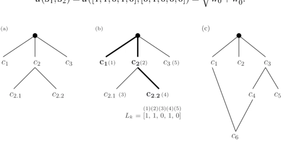
Figure 2.1: An example of dataset for hierarchical multi-label classification of functional genomics data.
The descriptive attributes present different aspects of the genes in the yeast genome, while the targets are protein functional classes organized hierarchically. (Stojanova et al, 2012).
Figure 2.1 gives an example of hierarchical multi-label classification. In particular, it presents an example dataset for hierarchical multi-label classification of functional genomics data. On the left part of the figure the targets, i.e., protein functional classes are presented in form of a tree (hierarchy structure). The hierarchy has three levels of classes. On the right part of the figure these same targets are presented as a binary vector. We can see that the targets that are given in bold in the hierarchy on the left are the ones that have values of one in the binary vector representation on the right, i.e., the one that actually appear in the given example. On the right part of the figure we also present the descriptive (discrete and continuous) attributes that describe different aspects of the genes in the yeast genome (Stojanova et al, 2012).
In contrast to classification and regression, where the output is a single scalar value, in this case the output is a data structure, such as a tuple or a Directed Acyclic Graph (DAG). This is also in contrast to the multi-target classification where each example is associated with a single label from a finite set of disjoint labels, as well as to multi-label classification where the labels are not assumed to be mutually exclusive: multiple labels may be associated with a single example, i.e., each example can be a member of more than one class.
These types of problems occur in domains such as life sciences (gene function prediction, drug discovery), ecology (analysis of remotely sensed data, habitat modeling), multimedia (annotation and retrieval of images and videos) and the semantic web (categorization and analysis of text and web). Having in mind the needs of the application domains and the increasing quantities of structured data, the task of “mining complex knowledge from complex data” was listed as one of the most challenging problems in data mining (Yang and Wu, 2006).
2.2
Relations Between Examples
When learning predictive models the i.i.d. assumption is violated in many real-world cases. Therefore, as we mentioned in the previous section, we consider the predictive modeling tasks without this assumption. Having defined a context space D that serves as a background knowledge and introduces additional information, related to the target space, and especially the distanced(·,·)on which it is defined, we can say that data is linked through some kind of relations. Moreover, they can be cases when this context space is not explicitly defined using dimensional variables, but only using a distance d(·,·) over the context space.
The relations that we consider are relations between the examples. They can be inherited from the data itself or artificially defined by the user, in order to substitute the missing natural ones or to enable some learning tasks to be accordingly addressed. We argue the use of these relations and emphasize the advantages of the used experimental settings which serve as a basis of our work.
Definition of the Problem 15
In the following Section, first we focus on the different types of relations that we consider. Then, we describe their origin. Finally, we explain their use within our experimental settings.
2.2.1 Types of Relations
Common machine learning algorithms assume that the data is stored in a single table where each example is represented by a fixed number of descriptive attributes. These are called attribute-value or proposi-tional techniques (as the patterns found can be expressed in proposiproposi-tional logic). Proposiproposi-tional machine learning techniques (such as the classification or regression decision trees discussed in the previous sec-tion) are popular mainly because they are efficient, easy to use and are widely accessible. However, in practice, the single table assumption turns out to be a limiting factor for many machine learning tasks that involve data that comes from different data sources.
Traditional classification techniques would ignore the possible relations among examples, since the main assumption on which rely most of the data mining, machine learning and statistical methods is the data independence assumption. According to this, the examples included in the learning process must be independent from each other and identically distributed (i.i.d.). However, examples of non i.i.d. data can be found everywhere: nature is not independent; species are distributed non-randomly across a wide range of spatial scales, etc. The consideration of such relations among example is related to phenomenon of autocorrelation.
The autocorrelation phenomenon is a direct violation of the assumption that data are independently and identically distributed (i.i.d.). At the same time, it offers a unique opportunity to improve the per-formance of predictive models on non i.i.d. data, as inferences about one entity can be used to improve inferences about related entities. We discuss this phenomenon in more details in the next Section 2.3.
The work presented in this dissertation differs from the propositional machine learning methods un-derlying the i.i.d. assumption. It introduces and considers autocorrelation that comes from the existence of relations among examples i.e., examples are related between each other. As mentioned in Section 2.1, this upgrades the setup of classical predictive modeling tasks it considers by introducing a context space
Dthat embraces these relations.
Such relations have already been considered in collective classification (Sen et al, 2008). It exploits dependencies between examples by considering not only the correlations between the labels of the ex-amples and the observed attributes of such exex-amples or the exex-amples in the neighborhood of a particular object, but also the correlations between labels of interconnected (or in a more general case we can say that there exists a reciprocal relation between the examples) examples labels of the examples in the neigh-borhood. In general, one of the major advantages of collective inference lies in its powerful ability to learn various kinds of dependency structures (e.g., different degrees of correlation (Jensen et al, 2004)).
Alternatively, even greater (and usually more reliable) improvement in classification accuracy can occur when the target values (class labels) of the linked examples (e.g., pages) are used instead to derive relevant relational features (Jensen et al, 2004).
Examples of collective classification can be found in the webpage classification problem where web-pages are interconnected with hyperlinks and the task is to assign each webpage with a label that best indicates its topic, and it is common to assume that the labels on interconnected webpages are correlated. Such interconnections occur naturally in data from a variety of applications such as bibliographic data, email networks and social networks.
The relations (dependencies) between examples are the most interesting and challenging problems in Multi-Relational Data Mining (MRDM) (Domingos, 2003). For example, molecules are not independent in the cell; rather, they participate in a complex chains of reactions whose outcomes we are interested in. Likewise, Webpages are best classified by taking into account the topics of pages in their graph neigh-borhood, and customers’ buying decisions are often best predicted by taking into account the influence