CTR/27/04 April 2004
Revisiting Lagrange Relaxation for Processing Large-Scale Mixed Integer Programming Problems
C Siamitros, G Mitra and C Poojari
Department of Mathematical Sciences and Department of Economics and Finance
Abstract
Lagrangean Relaxation has been successfully applied to process many well known instances of NP-hard Mixed Integer Programming problems. In this paper we present a Lagrangean Relaxation based generic solver for processing Mixed Integer Programming problems. We choose the constraints, which are relaxed using a constraint classification scheme. The tactical issue of updating the Lagrange multiplier is addressed through sub-gradient optimisation; alternative rules for updating their values are investigated. The Lagrangean relaxation provides a lower bound to the original problem and the upper bound is calculated using a heuristic technique. The bounds obtained by the Lagrangean Relaxation based generic solver were used to warm-start the Branch and Bound algorithm; the performance of the generic solver and the effect of the alternative control settings are reported for a wide class of benchmark models. Finally, we present an alternative technique to calculate the upper bound, using a genetic algorithm that benefits from the mathematical structure of the constraints. The performance of the genetic algorithm is also presented.
Table of Content
Abstract ... 1
1. Introduction and Background of MIP problems... 3
2. Literature review of Lagrangean Relaxation in processing MIP problems ... 4
3. Design of a general LR/MIP algorithm... 5
3.1 Relaxation of constraints ... 6
3.2 Determination of the Lagrange multipliers... 8
4. Implementing a generic LR/MIP solver... 11
4.1 Classification and Relaxation of the Constraints... 11
4.2 The Lagrange Multiplier ... 13
4.3 Structure of the generic solver... 16
4.4 Efficiency and Speed-up of the solver ... 19
5. Computational Results ... 20
5.1 Collection of test problems ... 20
5.2 Analysis of Results ... 24
6. Upper bound using Genetic Algorithm... 29
7. Discussions and Conclusions ... 33
8. References... 34
Appendix I: Constraint Classes ... 37
Appendix II: Detailed Computational Results ... 43
Revisiting Lagrange Relaxation for processing large-scale
Mixed Integer Programming problems
1. Introduction and Background of MIP problems
The availability of fast and reliable commercial solvers such as CPLEX[15], Xpress-MP[5], OSL[14] and FortMP[7], and the easy access to public domain solvers such as NEOS[27] and OSP[28], the processing of large-scale linear programming has become easier. The processing of Mixed Integer Programming (MIP) problems, however, still remains non-trivial and poses significant mathematical and computational challenges. During the past years, ‘branch and bound’ approach monopolised the commercial solvers for solving MIP problems. In the recent times, the limitations of exact optimisation methods became increasingly apparent, since many problems are too complex to be solved exactly and it is computationally expensive. Therefore, many commercial solvers have been enhanced by using improved cut generation techniques, or non-exact optimisation methods, or by using new techniques, like pre-processing. In this paper, we discuss the Lagrangean Relaxation (LR) decomposition technique, which is, from computational point of view, a well-established approach to solve structured problems.
In this paper, we utilise the existing knowledge of processing MIP problems using LR and thereby design an algorithmic framework for applying LR dynamically to different classes of MIP problems. The outline of the paper is as follows. In section 2 we review the existing literature and refer to the different problem domains, where LR based methods have been applied. In general the efficiency and the effectiveness of the implementation depends on how well the knowledge about the structure of the underlying problem has been exploited. In section 3 we discuss the general issues
while applying LR and in particular address the challenges while applying the method to process large-scale MIP problems. In section 4 we present the details of implementing a generic LR based solver. We explain the alternative classification of the constraints, techniques for updating the Lagrange multipliers, re-use of information over iterations. In section 5, we present the computational results on a selection of benchmark problems. Additionally, we compare the performances of different options of the solver. In section 6, we introduce a Genetic Algorithm as an alternative approach to calculate the upper bound of the models and we present some primarily results. Finally, in section 7, we discuss the outstanding issues and give directions for further research into the field.
2. Literature review of Lagrangean Relaxation in processing MIP
problems
Lagrangean Relaxation, also known as Lagrangean Decomposition, was introduced in the early 70’s through the pioneering work of Held and Karp[11][12] on the travelling salesman problem. It was discovered that the relationship between the systematic travelling-salesman problem and the minimum spanning tree problem yields a sharp lower bound on the cost of an optimum tour. Thereafter, Held et al.[13] tried to test the effectiveness of subgradient optimisation for approximating the maximum of certain pairwise linear concave functions. The results that they obtained were promising for applying the method to general large-scale linear programming problems. Subsequently, Geoffrion [9] in the mid 70’s developed a general theory for applying the method by exploiting special problem structures. Since then, many researchers worked in the field and tried to extend the current methodology [32][3][8] and to apply the method to different classes of Integer Programming (IP) and MIP problems of known structure. Mainly, most applications that can be found in the literature are based either on scheduling problems or on location problems.
Renato de Matta [29] used LR to find the schedule for producing products of a single level, capacitated line problem. The LR based approach that was used to solve the problem in question found near optimal solution faster than other exact optimisation methods. Kaskavelis and Caramanis [16] processed an industry size job-shop scheduling problem with more than 10000 resource constraints by using a
Lagrangean relaxation based algorithm. In their approach, they extended the algorithm by introducing two new features in the Lagrange multiplier updating procedure. Firstly, they replaced the dual cost estimation of all sub-problems and the update of the multipliers values by a surrogate dual cost function and a more frequent multipliers update. Secondly, they introduced an adaptive step size in the subgradient-based multipliers. Both of the added features produced a more robust algorithm with significant attenuated solution oscillations, better feasible schedules and faster convergence. Kobayashi et al. [24] extended the subgradient optimisation method for calculating the Lagrange multipliers and introduced an intelligent way of updating these multipliers. The computational results arise show that the suggested method is very effective in solving scheduling problems.
A wide variety of effective Lagrange relaxation applications to location problems were also designed [2][4][22][21][1][6][17][10][23][31]. One of the principal researchers in the field, Beasley, presented a framework for developing Lagrangean heuristics with respect to location problems[2]. These heuristics are based upon Lagrange relaxation and subgradient optimisation method for solving different types of location problems. The computational results presented, indicate that the suggested algorithmic framework is robust. In a similar application, Christofides and Beasley [4], attempted to improve the lower bound of capacitated location problem by using subgradient optimisation method.
Senne and Lorena [31], proposed the Lagrangean / Surrogate as an alternative relaxation, in order to correct the erratic behaviour of subgradient like methods. The proposed alternative approach was tested in p-median problems and from the computational results showed that Lagrangean/Surrogate relaxations are very stable (low oscillating) and are reaching equal quality results in less computational time than the Lagrangean alone heuristics.
3. Design of a general LR/MIP algorithm
Lagrangean Relaxation is a Price Directive decomposition technique[23], which in the first instance simplifies and reduces the problem in question by relaxing
groups of constraints. Lagrangean relaxation has been successfully used in processing many different instances of combinatorial optimisation problems, such as the Travelling salesman Problem [11], [3] and [22]. Many combinatorial optimisation problems consist of an easy problem that is complicated by the addition of extra constraints. Applying LR in these problems involves identifying these complicating constraints, and then relaxing them by attaching penalties to the complicating constraints and then absorbing them into the objective function. These penalties are known as the Lagrange multipliers. Due to the relaxation of the complicating constraints, the relaxed problem becomes much easier to solve. The next aim is to find tight upper and lower bounds to the problem by iteratively processing sequence of modified sub-problems.
LR involves addressing two important issues; one is a strategic issue and the other a tactical issue [3]. The strategic issue concerns the classification and relaxation of the constraints. The strategic question is of the form “What constraints are to be relaxed?” The tactical issue deals with the selection of a good technique for updating the Lagrange multipliers. The tactical questions are of the form, “How the reduced problem can be solved?” or “How can we calculate an efficient bound?”.
3.1 Relaxation of constraints
Before defining the general MIP problem, lets identify the following index sets:
B={1,…,|B|} Index set for binary variables, I={|B|+1,…,|B|+|I|} Index set for integer variables, C={|B|+|I|+1,…,|B|+|I|+|C|} Index set for continues variables,
N=B∪I∪C Index set for all variables.
{ }
I
j
iff
Z
x
B
j
iff
x
C
j
iff
R
x
n
l
g
x
b
m
k
d
x
a
t
s
x
c
j j j N j lj j l N j kj j k N j j j∈
∈
∈
∈
∈
∈
=
=
≥
=
=
≥
+ + ∈ ∈ ∈1
,
0
,...,
1
,...,
1
.
.
min
This initial problem P0 is known as the master problem. Since this master
problem is difficult to solve, we relax a set of constraints, CO∈[1,m], by attaching Lagrange multipliers (λk≥ 0). Then, this relaxed group of constrints are appended to
the objective function and forms the following Lagrange Lower Bound Problem (LLBP):
{ }
I
j
iff
Z
x
B
j
iff
x
C
j
iff
R
x
n
l
g
x
b
t
s
d
a
c
x
j j j N j l j lj m k k N j m k j k j j∈
∈
∈
∈
∈
∈
=
=
≥
+
−
+ + ∈ = ∈ =1
,
0
,...,
1
.
.
)
(
min
1 1 κ κλ
λ
The Lagrange multipliers, λk, penalise the violation of the corresponding relaxed
constraints introduced in the objective function. The selection of which set of constraints to be relaxed is a strategic issue and we address it in the later section.
After decomposing the master problem, we are interested in choosing the appropriate numerical values for the Lagrange multipliers (tactical issue) for the problem PL(λ). In particular, we are interested in finding the values for λ that gives the
(P0)
maximum lower bound. The Lagrange lower bound problem is also known as the Lagrange dual program.
{ }
∈
∈
∈
∈
∈
∈
=
=
≥
+
−
+ + ∈ = ∈ = ≥I
j
iff
Z
x
B
j
iff
x
C
j
iff
R
x
n
l
g
x
b
t
s
d
a
c
x
j j j N j l j lj m k k N j m k j k j j k1
,
0
,...,
1
.
.
)
(
min
max
1 1 0 κ κ λλ
λ
The best value for λk is calculated by applying iterative updating techniques to the
above system (PDual). There are two well-known techniques that have been widely
used: Subgradient Optimisation and Multiplier Adjustment. In this paper, however, we will focus on the subgradient optimisation technique.
The estimation of a good solution to NP-hard problems by using a non-exact method, like LR, does not depend only on the calculation of a good lower bound. It is equally important to calculate good solutions that are feasible and provide upper bounds to the master problem. We thus reduce the duality gap and provide tight bound for the optimal solution. The duality gap is defined as the relative difference between the lower bound and the upper bound. In ideal instances, the Lagrange lower bound is equal to the upper bound. The upper bounds are usually calculated by using a Lagrange Heuristic (LH) [3]. An instant of a LH algorithm is to take the LLBP solution vector and to attempt to convert it to a feasible solution vector to the master problem.
3.2 Determination of the Lagrange multipliers
There have been two main techniques that have been successfully applied for finding Lagrange multipliers in a wide variety of problem instances. These are the subgradient optimisation and the multiplier adjustment. Sub-gradient optimisation is (PDual)
an iterative procedure that, starting from an initial set of Lagrange Multipliers, attempts to improve the lower bound of the LLBP in a systematic way. Multiplier adjustment is also an iterative procedure, but modifies only one component of the multiplier in an iteration.
The literature and the experiences of the researchers in the field [3] suggest that subgradient optimisation is a preferable method to update the Lagrange multipliers for general discrete optimisation problems. Sub-gradient optimisation is straight forward to implement and can be applied without modifications for different problem instances. Multiplier adjustment is non-trivial and requires to be modified for different problems. Moreover, even the quality of the solution is better on using the sub-gradient technique. Therefore, in our attempt to apply Lagrangean Relaxation for general discrete optimisation problems, we have used subgradient technique for updating the Lagrange multipliers.
Algorithmic Framework of Subgradient Optimisation
Define Cj as the cost coefficient vector of the LLBP (PL(λ)). Hence,
− = ki k kj j j c a C λ
where j = 1,…, n (number of coefficients) and k = 1,…, m (number of constraints). The main steps that have to be followed to apply subgradient optimisation are set out below:
STEP1: Initialisation
Set π, which is a user-defined parameter, equal to 2. ( 0≤π≤2) Set the lower bounds to -∞, and the upper bounds UB, ZUB to +∞.
Set N_LR = 0 (number of Lagrange iterations). Initialise the Lagrange Multipliers λ.
STEP2: Calculate lower bound
Solve the LLBP (PL(λ)) for the current set of λk to obtain the solution vector Xj
and the lower bound ZLB. (ZLBt ={xˆj})
If the Zlb > LB, set LB= ZLB.
STEP3: Calculate upper bound
Apply a Lagrange Heuristic to find a feasible upper bound ZUB. If ZUB <UB,
set UB =ZUB.
STEP4: Update the multiplier
a. Calculate the Subgradients t k
G for current solution vector Xj.
If all Gi≤ 0 for each ‘≥’ constraint, then ZLB is feasible.
b. Define a scalar step size T.
c. Update the Lagrange Multipliers set
STEP 5: Stopping criteria a. π < 0.005 b. (UB - LB) = 0.0 c. 1( )2 =0 = m k t k G
If stopping rules as not satisfied then go to STEP 2.
The user-defined parameter, π controls the step size T. In the case wherein the lower bound did not improve for 30 consecutive iterations, we half this parameter. Generally speaking, the smaller the value of this parameter, the smaller is the oscillation of the resulted lower bound (ZLB). In fact, when the value of the π
parameter is small, we are trying to improve the lower bound by searching on the “neighbourhood” of the LB.
There are three termination conditions of the algorithm. The algorithm terminates when the user-defined parameter becomes very small (i.e. 0.005), or when the dual gap (UB-LB) is equal to zero, or when the sum of squares of all the subgradients is equal to zero ( 1( )2 =0
=
m k
t k
G ). The last termination condition implies that all the constraints are perfectly satisfied and therefore all the Slack variables of the model are equal to zero.
m k x a d Gt k kj j k = − =1,..., = − = m k t k LB UB G Z Z T 1 2 ) ( ) ( π m k TGt k t k t k+1 =max(0,λ + ) =1,..., λ (eq. 2) (eq. 3) (eq. 4)
4. Implementing a generic LR/MIP solver
In order to implement successfully a generic LR solver we needed to resolve the following questions:
1. How to calculate good upper and lower bounds? 2. Which constraints to relax?
3. How to initialise λ, and update the same?
In addition we wanted the scheme to be generic such that it can be applied to wide problem MIP classes with minimal modifications. During the course of our research we encountered problems such as in some instances, the λ vector was not updated as expected and the generated Lagrange Lower Bound Problem became unbounded and the execution of the algorithm could not continue. We next discuss our investigations into the strategic issue involved in relaxing the appropriate constraints and the tactical issues in updating the Lagrange multipliers.
4.1 Classification and Relaxation of the Constraints
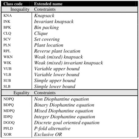
A constraint classification (CC) procedure [19][20] analyses the constraints of a given MIP problem and partitions them into different classes of known structure. As noted in [26], CC involves the identification of interesting special cases. There is no defined terminology and classification scheme in the literature. To classify constraints, we first distinguish binary variables from integer and continuous ones. All the linear constraints are analysed first one by one to see if they belong to any of our predefined well-known classes of constraints. The classified rows are taking into account several parameters. These parameters include the type of variable, the number of variables, the coefficient values, the type of bounds and the sense of the constraint. Using the above parameters the defined constraint classes are given in Table 1.
Table 1: IP constraint classes
In the above-defined classes some classes are subclasses of other defined classes when they satisfy certain properties. The mathematical presentations [19] of the above classes are defined in Appendix I.
One of the key issues for obtaining good lower bounds, when Lagrange Relaxation is applied, is the integrality property. As described by Beasley [3] and Geoffrion [9], a Lagrange Lower Bound Problem, like (PL(λ)) introduced above, is said
to have the integrality property when the solution of the relaxed problem is unchained, even after the integrality constraint, x∈(0,1), is replaced by its linear relation
1
0≤x≤ . Lagrange Lower Bound Problems for which this property holds can not result in a better lower bound than the LP relaxed solution of the master problem. Hence, this property can be expressed by the following constraint:
opt LR
LP Z Z
Z = ≤
when the integrality property holds, otherwise by:
Class code Extended name
Inequality Constraints
KNA Knapsack
INK Invariant knapsack BPK Bin packing
CLQ Clique
SCV Set covering PLN Plant location
RPL Reverse plant location WKN Weak (mixed) knapsack
WIK Weak (mixed) invariant knapsack VUB Variable upper bound
VLB Variable lower bound SUB Simple upper bound SLB Simple lower bound
Equality Constraints
NDPQ Non Diophantine equation
BDPQ Binary Diophantine equation
MDPQ Mixed Diophantine equation
IDPQ Integer Diophantine equation
DGOQ Discrete goal oriented equation
PFLD P-fold alternative
opt LR
LP Z Z
Z ≤ ≤
where Zopt is the optimal solution to the master problem, ZLRis the maxmin optimal solution to the LLBP and ZLP is the relaxed solution to the master problem.
In order to overcome this problem of integrality property and obtain lower bounds better than the relaxed solution we designed a simple Greedy Algorithm (GrA) to select an appropriate set of constraints to be relaxed. The design of this algorithm is based on the empirical observation that when all the constraints are relaxed or when the relaxed constraints are not independent, it is more likely the Lagrange relaxation problem to have the integrality property. The framework of this GrA is as follows. Initially, we apply the constraint classification routine in order to analyse the constraints that the model contains. Afterwards, we form a subset, CO, of constraint classes that we consider that are complicating the model and may be relaxed. From this subset of constraints, CO, we are trying to find the maximum number of “independent constraints”. By the term “independent constraints” we define the subset of constraints, COI ⊆CO, that do not contain a variable that is already contained in another constraint member of the subset COI. The constraints
that are not members of COI are classified as “dependent constraints” and are
members of the subset COD (CO=COI ∪COD). In order to form these two subsets
in a simple manner, we initially compute the total number of variables that each constraint of the set CO contains. Afterwards, starting from the constraint with the less number of variables, we start to insert new members to the subset COI until no
further independent constraints can be found in CO. This Greedy algorithm may not guarantees that we obtain the maximum possible number of independent constraints, but for some of the tested models of our research worked sufficiently. As it will be presented in following section, where the obtained results will be presented and analysed, the application of this GrA was effective on improving the lower bound of the LLBP.
4.2 The Lagrange Multiplier
Within the sub-gradient optimisation we have experimented with three alternative rules for updating the Lagrange multipliers. The first one is the conventional method
as described in the sub-gradient optimisation section above (section 3.2). The other two strategies of updating the multipliers are more sophisticated and are based on the work done by Kobayashi et al.[24]. In these approaches, instead of applying the same rule for updating each component of the Lagrange multiplier, different rules are used depending on conditions of the corresponding constraint. Briefly, these conditions are described below, where ‘k’ is the number of iterations and ‘i’ is the entry of the λ
vector:
If (t=1 or (Gkt-1>0 and Gkt>0)) then
λkt+1 = λkt + T × Gkt, βkt = T × Gkt
else if ((Gkt-1>0 and Gkt<0) or (Gkt-1<0 and Gkt<0)) then
λkt+1 = λkt – 0.5 | βkt-1 |, βkt = 0.5 βkt-1
else if (Gkt-1<0 and Gkt>0) then
λkt+1 = λkt + 0.5 | βkt-1 |, βkt = 0.5 βkt-1
else if (Gkt=0 or (Gkt-1≤0 and Gkt<0)) then
λkt+1 = λkt , βkt = 0
else use first condition.
As it is demonstrated in Kobayashi et al.[24], this approach of updating the λ vector reduces the oscillation of the solution and decreases the number of iterations.
We have extended the above idea. In cases where the consecutive values of two subgradients, Gk, are of opposite sign, (Gkt-1>0 and Gkt<0) or (Gkt-1<0 and Gkt>0),
we try to estimate the corresponding value of λkt such that Gkt+1 tends to zero. For
instance, suppose at the tth iteration the value of Gkt = 2, λkt = 0.0 and at the t+1
iteration Gkt+1 = -2 and λkt+1 = 1.0. Then, as the concept of our approach is illustrated
in (Figure 1), we the desired λ value is 0.5.
-2.5 -2 -1.5 -1 -0.5 0 0.5 1 1.5 2 2.5 0 0.1 0.2 0.3 0.4 0.5 0.6 0.7 0.8 0.9 1 lamda values S ub -g ra di en t
Figure 1, Two opposite sign subgradients
Briefly, the conditions of our approach are described below:
If (t=1 or (Gkt-1>0 and Gkt>0)) then
λkt+1 = λkt + T × Gkt, βkt = T × Gkt
else if (Gkt-1<0 and Gkt<0) then
λkt+1 = λkt – 0.5 | βkt-1 |, βkt = 0.5 βkt-1
else if ((Gkt-1>0 and Gkt<0) or (Gkt-1<0 and Gkt>0)) then
λkt+1 = λkt - Gkt×(λkt-1 - λkt) / (Gkt-1 - Gkt),
βkt = Gkt×(λkt-1 - λkt) / (Gkt-1 - Gkt)
else if (Gkt=0 or (Gkt-1≤0 and Gkt<0)) then
λkt+1 = λkt , βkt = 0
else use first condition.
In case we deal with a ‘≥’ constraint, if the corresponding multiplier turns out to be negative, its set to zero so that the Lagrangean Relaxation theory will not be violated.
In order to speed up the algorithm of updating the Lagrange multipliers of our generic solver, an optional feature is included; the subgradient adjustment algorithm [3]. This procedure involves setting the subgradient Gk of a ‘≥’ inequality constraint
to zero when the corresponding Lagrange multiplier is 0 and Gk is less than zero (Gk <
0). The reason for doing so is since λk will be zero, it is irrelevant to include Gk in
calculating the denominator in (eq. 3) of subgradient optimisation.
4.3 Structure of the generic solver
In the generic solver we address the important strategic and the tactical issue (see Figure 2). We found that both these issues are equally important for successfully processing large-scale models using LR.
Figure 2, Framework of generic Lagrange Relaxation based solver
The solver is divided in two parts, the pre-processing and the main Lagrangean iterations. The pre-processing involves the constraint classification and all the operations carried out before applying LR, like initialising the solver, selecting the sets of constraints to be relaxed, generating the arrays for the Lagrange Lower Bound Problem (LLBP) and the Upper Bound problem, initialising the dimension and the data for the models, generating the statistics and selecting the options to be used
Initialisation
L a g r a n g e I t e r a t i o n s
Update the Lagrange multipliers Strategic Issue Tactical Issue
P r e – p r o c e s s i n g
Classification and relaxation of constraintsby the solver. We used FortMP to solve the MIP problems for calculating the upper and lower bounds at each iteration. Initially, we identify the number of integer and binary variables in each constraint and then we classify the constraints into different classes. We use FortMPOT[19][20] for classifying the constraints and calculating the cardinality of the resulting class.
The statistics generated during the pre-processing phase is used to identify the potential constraints that could be relaxed. Based on the information the user could:
1) Provide the list of constraints that should be relaxed. This procedure can become extremely tedious for large models.
2) Alternatively, the user could specify the index of the constraints, within each of the constraint class that should be relaxed.
Because in some models during the testing processes it was observed that some lower bound sub-problems are unbounded, the use of aggregation constraints was considered. By selecting to add an aggregation constraint for each relaxed constraint set, most of the cases, where an unbounded sub-problem was arisen, were resolved. In order to be able to introduce aggregation constraint(s), it necessitates that at least two constraints of the same constraint set to be relaxed. After selecting the constraints to be relaxed, the LLBP is generated. Then, for computational purposes all the remaining ‘≤’ constraints of the LLBP are transformed into ‘≥’ constraints.
We next address the issue of initialising the Lagrange multiplier. We have experimented with 3 alternative choices. The first involves setting all the entries of the Lagrange multiplier vector equal to a preferable value (usually 0). The second choice, allows the user to initialise the values of the Lagrange multiplier vector one at a time. The third option sets the entries of the Lagrange multipliers to the dual values obtained by solving the master problem to the first integer solution. Furthermore, in case we have a ‘≥’ constraint and the corresponding dual value found is negative, then the dual value is set to zero, since it can take only non-negative values in such instances.
Next, we discuss the phase corresponding to the main Lagrangean iterations. During our investigations, it was observed that for some models, when many constraints were relaxed, the resulting LLBP become unbounded. We tried to resolve
this ‘unboundedness’ by adding aggregation constraints as described before. Such constraint aggregation resolves the issue of ‘unboundedness’ for some models, however, the quality of the lower bounds was not that good. Therefore, we constructed a procedure that half the values of the Lagrange multipliers repeatedly until the LLBP sub-problem becomes bounded. Theoretically, when all the Lagrange multipliers are zero, the sub-problem is bounded as far as the master problem is bounded and all the cost coefficients are positive in a minimisation problem.
For the calculation of the upper bound we designed a heuristic algorithm that computes the upper bound using the solution vector returned from the LLBP. The upper bound sub-problem is generated by fixing the values of the integer and binary variables to the solution resulted in the LLBP. Fixing of the variables reduces the dimension of the model and thereby the computational complexity of processing the same. We do not arbitrarily fix the integer and binary variables. Instead, we consider the constraints that have been relaxed to generate the LLBP and identify which of these constraints satisfy the inequality. Then, in the original problem we fix integer and binary variables arising only in such constraints. This condition for selecting which integer and binary variables should be fixed is important to ensure that a feasible solution may exist. In case we omit this condition and we have a non-satisfied relaxed constraint that contains integer and/or binary variables, then the generated upper bound sub-problem will become infeasible, since it contains all the sets of constraints. The generated upper bound sub-problem is solved not to optimality, but to feasibility. This feasible solution of the upper bound sub-problem is also a feasible or the optimal solution of the master problem. This heuristic is illustrated by mathematical formulation as follows:
Set of violated relaxed constraints
} ) int ' ' 0 int ' ' 0 ( |
{k G for constra s G for constra s k CO
V t k t k t CO = < ≥ ∨ ≠ = ∧ ∈
Set of indexes corresponds to binary variables to be fixed )} 0 ( | { t CO kj t F j j B a k V B = ∈ ∧ ≠ ∉
)} 0 ( | { t CO kj t F j j I a k V I = ∈ ∧ ≠ ∉
The corresponding upper bound problem to be solved is:
}
|
ˆ
{
,
\
,
\
}
1
,
0
{
,
,...,
1
,...,
1
.
.
min
t F t F t j j t F j t F j j N j lj j l N j kj j k N j j jI
j
B
j
x
x
I
I
j
iff
Z
x
B
B
j
iff
x
C
j
iff
R
x
n
l
g
x
b
m
k
d
x
a
t
s
x
c
∈
∨
∈
=
∈
∈
∈
∈
∈
∈
=
=
≥
=
=
≥
+ + ∈ ∈ ∈Finally, another optional feature was added in our generic solver called the best start for the Lagrange multiplier, which we found it speeds up the algorithm. This optional procedure has two alternatives. At the beginning of each outer iteration of the subgradient algorithm (when π is updated), the Lagrange multipliers vector will be set either to Lagrange multipliers vector that resulted when the best lower bound was obtained or to the Lagrange multipliers vector that resulted when the best upper bound was found so far. The concept of this procedure is to start the search in the next iteration set from a vector that returned the best result found so far.
4.4 Efficiency and Speed-up of the solver
The algorithm requires significant amount of house-keeping operations at each iteration, such as identify the sense of the constraints (that is ≥, ≤ & =) and the relaxed constraints. We have constructed the data structure so that such information are found with minimal search time. This requires us to store the auxiliary information and thus increases the memory requirement. But our experience shows that the resulting speed-up in processing the problem offsets the memory requirement.
An implementation of an efficient generic LR solver requires the algorithm to be not only mathematically sound, but also efficient in the computational implementation. We spend significant time and effort in the coding of the functions, implementing alternative version prior to concluding the most efficient one. Our goal was to reduce the number of floating point operations (flops) in the program. We found that there was a trade-off in the number of calculations that the program needs to perform versus the amount of information that is stored in the memory. The algorithm showed significant computational speed-up if repeatedly used information were stored for later use. For instance, at each iteration we need to identify the sense of each constraint in order to select rule for updating the Lagrange multipliers vector. Instead of searching the data matrices for the sense of each constraint at each iteration, an array was created that contains that piece of information. Another example of improving the performance of the program was in the calculation of the subgradients. Instead of repeatedly searching the matrices of the master problem to find the relaxed constraints in order to calculate the subgradients at the end of each iteration, the data values of the relaxed constraints were stored in a different set of matrices. This storage increases the memory required by the program, as more arrays have to be generated, but certainly we speed up the solver.
5. Computational Results
We test the performance of the generic Lagrange Relaxation algorithm by using alternative benchmark models. Moreover, we test the effect that the different controls have on these models. We compare the computational performance of our implementation with other solvers such as CPLEX, FortMP, Xpress, OSL, BonsaiG and GLPK.
5.1 Collection of test problems
The selected model collection was drawn from: 1) H. Mittelmann [25], 2) ZIP [18] and 3) MIPLIB3.0 [30]. The statistics of the selected models are presented in the table below (Table 2). This table contains the number of rows, including the objective
row, the number of columns, the number of integer and binary variables and the number of non-zero elements of each model.
Table 2, Model statistics of benchmark models
The table below, Table 3, illustrates the known solutions of the models, where the ‘IntSol’ and ‘LP Sol’ columns indicate the integer and linear solution of the model respectively.
Benchmark Model
Name rows col Int./Binary nonzero
10teams 231 2025 0/1800 14175 ran8x32 297 512 0/256 1536 ran12x21 286 504 0/252 1512 irp 40 20315 0/20315 118569 prod1 209 250 0/149 5351 bienst1 577 505 0/28 2185 bienst2 577 505 0/35 2185 swath1 885 6805 0/2306 34966 acc2 2521 1620 0/1620 15328 H . M itt el m an n acc5 3053 1339 0/1339 16135 air04 824 8904 0/8904 81869 air05 427 7195 0/7195 59316 l152lav 98 1989 0/1989 11911 misc07 213 260 0/259 8620 rentacar 6804 9557 55/0 42019 stein27 118 27 0/27 405 Z IP stein45 332 45 0/45 1079 vpm1 234 378 0/168 917 air06 826 8627 0/8627 79433 M IP L IB 3. 0 p6000 2177 6000 0/6000 54238
Benchmark Model
Name IntSol LP Sol
10teams* 924 917 ran8x32* 5247 4937.5845 ran12x21* 3664 3157.3774 Irp* 12159.493 12123.5302 prod1* -56 -100 bienst1 46.75 11.7241 bienst2* 54.6 11.724138 swath1* 379.069 334.4969 acc2* 0 0 H . M itt el m an n acc5* 0 0 air04* 56138 55535.436 air05* 26374 25877.609 l152lav* 4722 4656.36 misc07 2810 1415.0 rentacar* 30356761 28806137.64 stein27 18 13.0 Z IP stein45* 30 22.0 vpm1* 20 15.4167 air06* 49649 49616.364 M IP L IB 3. 0 p6000* -2451377 -2451537.325
Table 3, Integer and LP solution of models
In the following two tables, Table 4a and Table 4b, the time taken by different solvers to solve the selected models is illustrated. All the models were run in default mode for each solver except CPLEX for which "mipgap" was decreased to 1.e-5 from 1.e-4 and FortMP for which specially tuned control settings were used. The computational experiments were carried out on a Pentium 4 (1.5 GHz, 1GB RDRAM, Linux-2.4.18)[25], except those of FortMP, which were run on a Pentium 4 (2.4GHz, 1GB DDR-RAM, Win2000). The column ‘Best FortMPSol’ denotes the best solution found by FortMP.
Benchmark Model
Name FortMP (sec) CPLEX (sec) -MP (sec) XPRESS OSL (sec) FortMPSol Best
10teams* 1351.4 78 154 >10000 926 ran8x32* 29.2 47 321 >15000 5382 ran12x21* 25.6 629 16859 >15000 3744 Irp* 3600 9 32 380 12159.493 prod1* 17.8 234 >30000 >10000 -40 bienst1 538 891 2228 3744 46.75 bienst2* 995.6 12865 12906 >20000 55.5 swath1* 708 250 16 41 379.0713 acc2* ----** 412 542 144 ---- H . M itt el m an n acc5* ----** 2174 2958 >10000 ---- air04* 3600 133 435 >10000 56576 air05* 3600 180 1110 498 26456 l152lav* 690.2 4 101 75 4722 misc07 241 260 185 122 2810 Z IP stein45* 79.05 54 131 376 30
Table 4a, Solution times of models by all solvers
Benchmark Model
Name FortMP (sec) FortMPSol Best
rentacar* 586 29888573 stein27 5 18 Z IP vpm1* 36.6 20 air06* 264 49649 M IP L IB 3. 0 p6000* 2477 -2449956.2
*Integer solution found so far; Termination conditions of FortMP solver reached **FortMP solver couldn’t find a single feasible solution
Table 4b, Solution times of models by FortMP
In the Table 5 below, the constraints of each model were classified. The abbreviations of the IP constraint classes are defined in Table 1.
Model
Name INK CLQ PFLD XOR VUB NDPQ KNA OLE MLE BPK DGOQ SLB RNG SCV
10teams 45 50 15 120 - - - - ran8x32 - - - - 256 40 - - - - ran12x21 - - - - 252 33 - - - - irp - - - 39 - - - - prod1 - - - 7 100 1 100 - - - - bienst1 - - 4 - 196 124 - 252 - - - - bienst2 - - 5 - 245 123 - 203 - - - - swath1 - - 189 - - 314 - 247 133 - - - - - acc2 387 1458 27 252 - - - 396 H . M itt el m an n acc5 455 1938 33 244 - - - 382 air04 - - - 823 - - - - air05 - - - 426 - - - - l152lav - - 1 95 - - 1 - - - - misc07 42 3 27 7 - - 3 - - 2 1 - - 127 rentacar - - 19 - - 6273 - 478 - - - 31 2 - stein27 1 - - - 117 Z IP stein45 1 1 - - - 329 vpm1 - - - - 168 42 - 24 - - - - air06 - - - 825 - - - - M IP L IB 3. 0 p6000 - 2046 - 123 - - 7 - - - -
Table 5, Constraint Classification of models
5.2 Analysis of Results
In order to test the performance of the generic solver, computational tests using different settings were carried out on several models presented in Table 2. Through this study, our aim was to identify the controls that are best suited. In order to rank different controls and analyse the quality of the results, we defined the following metric. 1 ) ,
max(
+ − =Z
Z
Z
Z
LP LB LB UB ε (eq. 5)where ZUB is the upper bound solution, ZLB is the lower bound solution and ZLP is the
relaxed solution. In perfect instances, where the lower bound is equal to the upper bound, the value of the metric, ε, becomes zero. Otherwise, in general the closer is the value of the metric to zero, the better is the quality of our result. The controls used for each model across all the experiments carried out are summarised in Table 6.
Table 6, Settings used across all experiments
‘Instant ID’ is the ID of the each control parameters set. ‘SG’ denotes that the classical sub-gradient optimisation algorithm was used to update the Lagrange multipliers. ‘ExtSG1’ symbolises that the extended sub-gradient algorithm, based on the work of Kobayashi et al [24], presented in section 4.2 was used. ‘ExtSG2’ indicates that our approach on extending the above idea was used to update the Lagrange multipliers.
Using the control settings of Table 6, we carried out three sets of experiments. Initially, we found the set of constraints that is complicating each model and we relaxed all the constraints of that set. The best instances obtained from this experiment are summarised in Table 7, where ‘Instant ID’ refers to the control parameters set in Table 6.
Instant
ID strategy Lamda Subgradient Adjust Algorithm
Best Lamda
Vector Option Starting Lamda
1 SG YES NONE 0.0
2 SG YES NONE 0.5
3 SG YES LB 0.5
4 SG YES UB 0.5
5 ExtSG1 YES NONE 0.0
6 ExtSG1 NO NONE 0.5 7 ExtSG1 NO LB 0.5 8 ExtSG1 NO UB 0.5 9 ExtSG2 NO NONE 0.0 10 ExtSG2 NO NONE 0.5 11 ExtSG2 NO LB 0.5 12 ExtSG2 NO UB 0.5
* Aggregation constraint was used
Table 7, Best results by relaxing all constraints of a certain type and warm-start B&B
As it can be observed by comparing the results obtained by the LR solver in Table 7 with the known solution of the models in Table 3, the best upper bound achieved by LR is close to the optimal solution. In two instances, ‘stein27’ and ‘vpm1’ model, the upper bound found is equal to the optimal solution. Furthermore, when the best found solution by LR was used to warm-start the Branch-and-Bound (B&B) algorithm, the value of the upper bound was further improved in almost all the instances. Unfortunately, in the set of experiments the quality of the lower bound was not that good and only in one case, ‘misc07’ model, the lower bound was better than the known LP relaxed solution. As it was discussed above, this is an issue of the integrality property. In order to attempt to overcome this problem and attain better lower bounds, we carried out a set of experiments, where the constraints were relaxed according the Greedy Algorithm presented in previous section. The best instances obtained from this experiment are summarised in Table 8, where ‘Instant ID’ refers to the control parameters set in Table 6.
Model
name Instant ID BestLB BestUB solution LR time(sec)
εεεε BestUB
by B&B solution B&B time(sec) 10teams 1 908.802 924 705 0.0166 924 205 bienst1 1 9.38636 47.8 51 3.0190 47 100 bienst2 4 6.54243 55.8571 54 3.8757 55.7333 100 bienst2* 8 9.32143 55.7333 36 3.6476 55.7333 100 l152lav 11 4008.04 4750 404 0.1593 4734 150 misc07 1 1614.16 3130 353 0.9385 2810 100 prod1 8 -99.429 -50 125 0.4950 -55 12 Ran12x21 1 2772.81 4102 1.6 0.4208 3744 21 ran8x32 1 4448.14 5738 1.9 0.2612 5382 22 stein27 7 13 18 2.8 0.3571 18 2.2 stein45 11 22 31 2.9 0.3913 31 8.4 vpm1 2 15.4105 20 1.5 0.2796 20 5.4
* Aggregation constraint was used
Table 8, Best results using Greedy Algorithm and warm-start B&B
By analysing the results of Table 8, it can be observed that in four models, ‘bienst1’, ‘l152lav’, ‘misc07’ and ‘stein27’, the lower bounds were significantly improved and except ‘l152lav’ model the integrality property problem was resolved. Unfortunately, for the remaining of the models, the results are not better than in the first experiment. This is due to the relaxation of only few constraints that the result in the formed LLBP not to be simplified sufficiently. Therefore, the external solver, FortMP, used to solve the LLBP at each iteration did not obtain high-quality lower bounds. In some instances, the limits of the generic LR solver or the external FortMP solver were reached and the process was terminated.
In the third set of experiments carried out, we attempted to use LR only as a booster to warm-start the B&B algorithm. Therefore, we reduced the number of iterations and the time limit of the generic LR based solver. The summary of the results obtained is presented in Table 9, where ‘Instant ID’ refers to the control parameters set in Table 6.
Model
name Instant ID BestLB BestUB solution LR time(sec)
εεεε BestUB
by B&B solution B&B time(sec) 10teams 2 0 940 204 1.0240 924 1004 bienst1 6 46.2 52 1339 0.1229 47 100 bienst2 3 0 65 365 5.1084 55.7333 100 bienst2* 9 0 62.6 362 4.9198 55.7333 100 l152lav 2 4542.63 4774 432 0.0497 4724 130 misc07 11 2460 3060 377 0.2438 2810 100
prod1 4 -∞ -50 301 -- Not Started
Ran12x21 1 2772.81 4102 1.6 0.4208 3744 21
ran8x32 1 4448.14 5738 1.9 0.2612 5382 22
stein27 5 15 19 10 0.2500 18 2.3
stein45 6 20.9178 32 259 0.4818 30 10
* Aggregation constraint was used
Table 9, Best results using LR as a booster to warm-start B&B
As it is noticeable by analysing the results in Table 9, even though the sum of the solution time of LR and B&B is significant less than in the previous sets of experiments, the best solution found is not worst. However, in some models like ‘bienst1’ and ‘l152lav’ the best solution found is better than in the previous experiments. The explanation of this fact is that the generic LR solver obtains a good upper bound at early iterations and thereafter is trying to improve it. While the solver is trying to improve its current best found solution, in some cases is moving to the wrong direction and is trapped in a worst local optimum. The complete set of results of all three experiments is presented in Appendix II.
In Appendix III, we present some graphs that illustrate the improvement of the bounds over the solution time. Figure A1, shows how the lower and upper bounds found are approaching the LP relaxed and optimal known solutions respectively. Similarly, in Figure A2 and Figure A3, are improving over the time and tend to the optimal solution. In Figure A4, the LLBP of the instant of model ‘misc07’ has not the integrality property, and therefore the solver finds successfully a better lower bound than the LP relaxed solution. Finally, in Figure A5, the generic LR based solver managed to improve the bounds of the ‘vpm1’ model rapidly.
Model
name Instant ID BestLB BestUB solution LR time(sec)
εεεε BestUB
by B&B solution B&B time(sec) 10teams 3 827.673 924 273 0.1049 924 204 bienst1 8 4.33679 50 8.8 3.5887 46.75 100 bienst2 5 4.1571 58.1111 9 4.2403 55.7333 100 bienst2* 9 9.32143 59 8.4 3.9043 55.7333 100 l152lav 10 3834.44 4748 315 0.1962 4724 127 misc07 2 1544.5 3290 113 1.1294 2810 100 prod1 12 -100 -50 3.4 0.4950 -55 10 ran12x21 5 2417.12 4102 0.2 0.5335 3744 21 ran8x32 6 4008.64 5738 0.2 0.3502 5382 21 stein27 7 13 18 0.09 0.3571 18 1.8 stein45 11 22 31 0.2 0.3913 31 6.8 vpm1 8 14.4376 20 0.2 0.3388 20 5.3
6. Upper bound using Genetic Algorithm
After analysing the results of the generic LR based solver, we focus on improving further the upper bound. Since most of the models consist of binary variables, we designed a dynamic Genetic Algorithm (GA) based solver, which extracts information from the structure of the constraints. The structure of general GA is as follows. Initially a set of solutions has to be generated randomly, where the members may not be feasible or accepted solutions to the problem. This set is known as population. The generated solutions are represented by chromosomes and are assessed before forming a new population. The evaluation of the solutions is made by the fitness function. Afterwards, chromosomes are selected according to their fitness value to form pair. From each pair, two new chromosomes are generated known as offsprings. After evaluating the new generated chromosomes, a new population is formed that contains the fittest chromosomes. In this fashion, good characteristics are spread throughout the population over the generations. This process is repeated until a very good solution is found or until all the solutions (chromosomes) converge to one solution. The idea of GAs is to recombine chromosomes in order find a chromosome that minimises the fitness function. The search for such a chromosome is based mainly on the recombination of “fitter” chromosomes of the population, without ignoring the rest of the chromosomes, in order to avoid to be trapped in local optima. The GA has four main issues concerning its successful implementation that are coding, the fitness function, parent selection and reproduction. A detailed description of these issues can be found in any textbook of GAs.
The philosophy of the dynamic GA that we implemented is to use LR to create the initial population and to split the chromosome into smaller sub-chromosome of fixed size though the whole procedure. In order to define the size of the sub-chromosomes, we used a Greedy Algorithm described in previous section to identify a set of independent constraints. From the set of these constraints, we selected all the binary variables of each constraint to form the sub-chromosomes. Since each set of binary variables should satisfy the constraint that were emerged from, we decided not to create the initial population randomly, but make use of the existing knowledge. This knowledge was procured by applying LR. By generating the LLBP without relaxing the set of independent constraints found by the Greedy Algorithm, we know
that the resulting solution vector is a feasible instance for the members of each sub-chromosome. Therefore, we generated an initial population that contains values that do not violate a subset of constraints, set of independent constraints, of the model to be solved. By using information obtain from the structure of the constraints, we try to speed-up the GA and find feasible solutions to the master problem in a more meaningful manner. The GA forms a new population by using mainly a crossover operation. Instead of selecting a pair of chromosomes to generate two new offsprings, our designed GA is selecting randomly a triple of chromosomes and by applying randomly crossover at the defined sub-chromosomes is generating three new offsprings. Furthermore, in order to ensure that the algorithm is complete and explores more solution spaces, we introduce an operation that is swapping randomly two genes within a sub-chromosome. To evaluate the fitness of each chromosome, we use an external solver, FortMP, to solve the master problem when the binary variables are fixed to the value of the chromosome. The pseudo-code of our GA is illustrated in Figure 3 below.
_____________________________________________________________________ Pre-processing (same as in LR based solver)
GA procedure
Analyse constraints and select set of constraints to form sub-chromosomes. Initialise arrays that store information related to the GA iterations.
Use information of analysed constraints to define sub-chromosomes. Use external solver to find first feasible solution of model.
Use feasible solution to update initial Population. Initialise LR
pi = 2
select starting λ vector
(Populate GA’s initial Population of default size 20+1) while iteration number <= 20
Solve LLBP to optimality.
Use solution vector of LLBP to update initial population of GA. Calculate fitness of updated Population.
Start GA iterations
while GA iteration < Max set number
Select randomly three Chromosomes from Population matrix.
while iteration <= (20+1)/3
Randomly Crossover the sub-chromosomes of the three selected Chromosomes.
Calculate fitness of the three generated Chromosomes Update Population. (keep three best Chromosomes)
while iteration <= Max Swap Number (default 3) For all selected triples do
Select randomly to swap two genes of random selected sub-chromosome. Calculate fitness.
Update Population.
Display Best found Chromosome.
_____________________________________________________________________ Figure 3, Genetic Algorithm Pseudo-code
The testing and analysis of the GA is currently at an early stage. Therefore, only preliminary results are presented, which are very promising. The GA was used as a booster to the B&B algorithm for ‘bienst1’ and ‘bienst2’ model, where in both cases the best solution found by the GA is also the known optimal solution to the model. The solution time of the GA in both instances is extremely small. Especially, for the ‘bienst2’ model the GA managed to find the optimal solution in 144 seconds, when the industrial solvers require hundred of seconds to find a feasible solution and a few thousands of seconds to solve it to optimality (Table 4a).
Sub-chrom. Max genes per sub-chrom. Best feasible Solution by GA GA Solution time(sec) Best Solution by B&B B&B Solution time(sec) bienst1 4 7 46.75 153 46.75 100 bienst2 5 7 54.6 144 54.6 100
Table 10, Primarily results using GA as a booster to warm-start B&B
The following two figures, Figure 3 and Figure 4, illustrate the time needed to update the current best solution in the two solved model. As it can be observed, when these two figures are compared with Figure A2 and Figure A3 in the Appendix II, the genetic algorithm finds a better upper bound and faster.
bienst1 model 0 10 20 30 40 50 60 70 80 0 50 100 150 200 250 time bo un ds Optimal Solution LP rel. Solution
Figure 3, “bienst1” model iterations when GA was used as a booster to warm-start B&B
bienst2 model 0 10 20 30 40 50 60 70 0 50 100 150 200 250 time bo un ds Optimal Solution LP rel. Solution
Figure 4, “bienst2” model iterations when GA was used as a booster to warm-start B&B
Even though, the designed dynamic GA is highly based on information that can be extracted from the constraint structure of the model, the obtained results are ideal. Hence, we will try to improve further the algorithm and to apply it in different instances to monitor its behaviour.
7. Discussions and Conclusions
In this paper, we revisited the use of Lagrange Relaxation for processing combinatorial optimisation problems. We discuss issues related to the implementation of LR as a generic solver for processing large-scale MIP problem. By introducing some novel alternative strategies for updating the Lagrange multipliers vector and a heuristic for calculating the upper bound, we improve the solver performance. A feasible solution of the upper bound is calculated very fast, since the upper bound sub-problem is not solved to optimality in every iteration. In addition, as the lower bound approaches the upper bound, it is more than likely the variables of the upper bound sub-problem that will be fixed, will lead to an improvement of the current upper bound solution. A Greedy Algorithm was presented that is capable of resolving
in some instances the integrality property problem, this in turn lead to the improvement of the lower bound. The importance of constraint classification for selecting the sets of constraints to be relaxed has been emphasised. This generic LR solver provides the flexibility of adopting alternative strategies in the choice of the constraints to relax and updating the multipliers.
The generic solver was tested by solving a collection of benchmark problems using different control settings of the solver. The computational results obtained are promising, but further work has to be done on the calculation of the upper bounds. An alternatively procedure is introduced, which uses a dynamic genetic algorithm for calculating upper bounds. The dynamic Genetic Algorithm extracts information from the constraint structure of the model and uses Lagrange Relaxation to populate the initial population. The preliminary results obtain are very encouraging, but further analysis and testing are required.
8. References
[1] T. Aykin, (1994), Lagrangian relaxation based approaches to capacitated hub-and-spoke network design problems, European Journals of Operational Research, 79, 501-523.
[2] J.E.Beasley, (1993), Lagrangean heuristics for location problems, European Journals of Operational Research, 65, 383-399.
[3] J.E. Beasley, (1993), Lagrangean relaxation, In "Modern heuristic techniques for combinatorial problems" (C.R. Reeves, ed), 243-303, Blackwell Scientific Publications.
[4] N. Christofides and J.E. Beasley, (1983), Extensions to a Lagrangean
relaxation approach for the capacitated warehouse location problem, European Journals of Operational Research, 12, 19-28.
[5] Dash Optimisation, Xpress-Optimiser Reference manual, http://www.dashoptimization.com
[6] B. Dorhout, (1995), Solution of a tinned iron purchasing problem by Lagrangean relaxation, European Journal of Operational Research, 81, 597-604.
[7] E. F. D. Ellison, M. Hajian, H. Jones, R. Levkovitz, I. Maros, G. Mitra and D. Sayers, Optirisk Systems, FortMP Reference manual, http://www.optirisk-systems.com/
[8] M. Fisher, (1981), Lagrangian Relaxation Method for Solving Integer Programming Problems, Management Science, Vol. 27, No. 1.
[9] A.M. Geoffrion, (1974), Lagrangean relaxation for integer programming, Mathematical Programming Study, 2, 82-114.
[10] M. Guignard, (1988), A Lagrangean dual ascent algorithm for simple plant location problems, European Journals of Operational Research, 35, 193-200. [11] M. Held and R.M. Karp, (1970), The Traveling Salesman problem and
minimum spanning trees. Ops.Res., 18, 1138-1162.
[12] M. Held and R.M. Karp, (1971), The Traveling Salesman problem and minimum spanning trees: Part II. Math.Prog., 1, 6-25.
[13] M. Held, P. Wolfe and H.P. Crowder, (1973), Validation of subgradient optimisation, Mathematical Programming, 6, 62-88.
[14] IBM, OSL Reference manual, http://www.research.ibm.com/osl/ [15] ILOG, CPLEX Reference manual, http://www.ilog.com/products/cplex/ [16] C. Kaskavelis and M. Caramanis, Application of a Lagrangian Relaxation
Based Algorithm to a Semiconductor Testing Facility, Proceedings of the 4th Intnl. Conference on Computer Integrated Manufacturing and Automation Technology, Troy, NY, October 10-12 1994.
[17] A. Klose, (1998), Obtaining Sharp Lower and Upper Bounds for Two-Stage Capacitated Facility Location Problems. In: B. Fleischmann, J.A.E.E. van Nunen, M.G. Speranza, P. Stähly (eds.), Advances in Distribution Logistics, Lecture Notes in Economics and Mathematical Systems 460, pp. 185-214, Springer, Berlin Heidelberg New York.
[18] Konrad-Zuse-Zentrum für Informationstechnik Berlin
ftp://ftp.zib.de/pub/Packages/mp-testdata/ip/miplib/index.html
[19] K. Kularajan, (2000), Analysis of Integer Programming Problems and Development of Solution Algorithms, PhD Thesis, Brunel University, London.
[20] K. Kularajan, G. Mitra, E. F. D. Ellison and B. Nygreen, (2000), Constraint Classification, Preprocessing and a Branch and Relax Approach to Solving
Mixed Integer Programming Models, International Journals of Mathematical Algorithms, vol. 2, 1-45.
[21] C.Y. Lee, (1996), An algorithm for a two-staged distribution system with various types of distribution centers, INFOR, vol.34,no.2, 105-117.
[22] C. Lucas, S.A. MirHassani, G. Mitra and C.A. Poojari, (2001), An application of Lagrange relaxation to a capacity planning problem under uncertainty, Journals of the Operational Research Society, 52, 1256-1266.
[23] T.L. Magnanti and R.T. Wong, (1990), Decomposition Methods for Facility Location Problems. In: P. B. Mirchandani and R. L. Francis, Discrete Location Theory, Wiley-Interscience Series in Discrete Mathematics and Optimization, p. 209-262, John Wiley & Sons.
[24] Minoru Kobayashi, Takuya Yamaguchi, Kenji Muramatsu (2000), Updating of the Multiplier in the Lagrangean Decomposition Coordination Method of Scheduling Problems, Proceedings of the 1st World Conference on Production and Operations Management (CD-ROM Version), File Name=1161.pdf. [25] H.D. Mittelmann, Arizona State University ftp://plato.la.asu.edu/pub/milpc.txt [26] G.L. Nemhauser, M.P.W. Savelsbergh and G.C. Sigismondi, (1992),
Constraint Classification for Mixed Integer Programming Formulations, COAL Bulletin-Committee on Algorithms of Mathematical Programming Society 20, 8-12
[27] NEOS, http://www-neos.mcs.anl.gov/neos/ [28] OSP, http://www.osp-craft.com/
[29] Renato de Matta (1994), A Lagrangean Decomposition Solution for the Single line Multiproduct Scheduling Problem, European Journal of Operational Research, Vol 79, pp. 24-37.
[30] RICE University (MIPLIB 3.0)
http://www.caam.rice.edu/~bixby/miplib/miplib_prev.html
[31] E.L.F. Senne and L.A.N. Lorena, (2000), Lagrangean/Surrogate Heuristics for p-Median Problems. In: Computing Tools for Modeling, Optimization and Simulation: Interfaces in Computer Science and Operations Research, M. Laguna and J. L. Gonzalez-Velarde (Eds.), Kluwer Academic Publishers, pp. 115-130.
[32] J.F. Shapiro, (1979), Mathematical Programming: Structures and Algorithms, Wiley-Interscience.
Problem Definition [20]
Lets consider the Index sets, Data parameters and the Decision variables defined below:
Index sets
B={1,…,|B|} Index set for binary variables, I={|B|+1,…,|B|+|I|} Index set for integer variables, C={|B|+|I|+1,…,|B|+|I|+|C|} Index set for continues variables,
N=B∪I∪C Index set for all variables,
K=I∪C Index set for integer and continues variables. Data parameters
Lj, uj, cj, aij, bi are given values.
Decision variables xj∈ {0,1},
and xj = (1-xj) ∈ {0,1}, j ∈ B.
other bounded variables xj∈ Z, j ∈ I,
xj∈ R, j ∈ C,
lj≤ xj≤ uj, j ∈ K.
For a general MIP problem of the form:
The binary variable set B is further divided for row i as follows
i ij i ij i i i B j j B and a B j j B and a B B B + − + − = ∈ > = ∈ < = ∪ { | }, { | }, . 0 0
This means that:
B B i i = ∪( ). Similarly, i ij i ij i i i K j j K and a K j j K and a K K K + − + − = ∈ > = ∈ < = ∪ { | }, { | }, . 0 0 This means that:
K K i i = ∪( ). m i b x a t s x c N j ij j i N j j j ,..., 1 . . min , = ≥ ≤ ∈ ∈