Volume 5 - Article 2 | Pages 23–64

in the population sciences published by the Max Planck Institute for Demographic Research Doberaner Strasse 114 · D-18057 Rostock · GERMANY www.demographic-research.org

DEMOGRAPHIC RESEARCH

VOLUME 5, ARTICLE 2, PAGES 23-64

PUBLISHED 24 SEPTEMBER 2001

www.demographic-research.org/Volumes/Vol5/2/

DOI: 10.4054/DemRes.2001.5.2

On the impossibility of inferring cohort

fertility measures from period fertility

measures

Evert van Imhoff

1. Introduction 24

2. Period and cohort quantum: are they related? 25

3. Approaches to infer cohort TFR from period TFR 26

3.1 Period TFR 26

3.2 Approach 1: demographic translation 30 3.3 Approach 2: period adjustment 30 3.4 Approach 3: period extrapolation to complete

censored cohorts

33

3.5 Conclusion for cohort quantum 36

4. An empirical analysis of cohort fertility trends in the Netherlands and Italy

36

4.1 Data 36

4.2 Period trends and B-F adjustment 37 4.3 Looking at cohort quantum directly 42

5. Conclusions 56

6. Acknowledgements 56

Notes 57

References 58

On the impossibility of inferring cohort fertility

measures from period fertility measures

Evert van Imhoff 1

Abstract

A particularly important struggle faced by demographic analysts is, how to arrive at statements about family formation processes from a cohort perspective from data that are essentially collected on an annual basis. The present paper is concerned with this struggle, mostly restricted to the case of fertility. The central question investigated here is: given observed period data, what can we conclude about the completed family size of real women? I review several existing methods to infer cohort fertility from period fertility measures. The conclusion is that, for each method, its justifiability can be verified only empirically: by looking at cohort fertility directly. To illustrate how this can be done, the paper analyses fertility data from a cohort perspective for two countries, Italy and the Netherlands.

1 _{Netherlands Interdisciplinary Demographic Institute (NIDI), P.O. Box 11650, 2502 AR The Hague,}

1. Introduction

Each time demographers use the term ‘quantum of fertility’, they refer to the level of fertility, in some sense. They ask themselves: what is the current level of fertility? And what will it be in the future? And why?

I am a fervent subscriber to the concept of relativity: the measurement of a phenomenon depends on the perspective of the observer. What do we mean by ‘the level of fertility’? We mean something like ‘how many children do people have, on average’. But what is our perspective? I see two fundamentally different perspectives here, which should be familiar to anyone acquainted with the Lexis diagram:

1. The period perspective, i.e. looking at the reproductive behaviour of the total population. In my view, the ultimate indicator for the period quantum of fertility is the annual number of births (relative to the total population size, i.e. the crude birth rate). It is this indicator that tells us all there is to tell about what is happening today in the reproduction department. It also tells us (almost; we also need migration and mortality) all there is to tell about how our future pensions are to be taken care of.

2. The cohort perspective, i.e. looking at the reproductive behaviour of the individual members of the population. In my view, the ultimate indicator for the cohort quantum of fertility is the cohort net reproduction rate, or the cohort completed family size, in short: the average number of children a typical person produces over the course of his/her life time. This indicator tells us all there is to tell about how today’s people are reproducing themselves. It also tells us (almost; we also need adoption, and reconstituted families, and mortality) all there is to tell about what our future kinship patterns look like.

In principle, these are two fundamentally different concepts of the quantum of fertility. Obviously, there exists some relation between the two (after all, both refer to the same set of babies and mothers), but the exact relationship depends on so many factors that a sensible starting point is to treat them as fundamentally different. Many demographic arguments are flawed (particularly, but unfortunately not exclusively when made by non-demographers) because the two concepts are thought to be one and the same thing. So it is better to start by saying they are different (and later add a few similarities) than to start by saying that they are the same (and forget to add a few crucial differences).

basis, i.e. from a period perspective. The present paper is concerned with this struggle, mostly restricted to the case of fertility. The central question investigated here is: given observed period data, what can be conclude about the completed family size of real women? My conclusion will be: in practice we can say very little. The only way of finding out how cohorts reproduce themselves, is to look directly at fertility data from a cohort perspective.

The structure of this paper is as follows. Section 2 contains some general remarks about the relation between period and quantum indicators. In section 3, I will review several existing methods to infer cohort fertility from period fertility measures. The conclusion is that, for each method, its justifiability can be verified only empirically: by looking at cohort fertility directly. To illustrate how this can be done, section 4 analyses fertility data from a cohort perspective for two countries, Italy and the Netherlands. The final section summarizes and concludes.

2. Period and cohort quantum: are they related?

The main factors linking period and cohort quantum are threefold: (1) the age composition of the population; (2) the age pattern of fertility (sometimes denoted as the ‘tempo’ of fertility; personally I think the French word ‘calendrier’ is much more accurate); (3) changes over time in (1) and (2).

Under ideal circumstances (I mean: circumstances that exist in theory only), it is possible to derive relationships between period and cohort quantum indicators, conditional on timing and age composition factors. This provides very useful insights in the underlying demographic mechanisms. However, in real life the factors involved in explaining the link between period and cohort quantum are so complex and subtle, that it is my firm belief that we will never be able to describe it completely. Even with many data and a complicated model, I believe we cannot accurately derive cohort indicators from period indicators or vice versa. At best, we can derive evidence for supporting qualitative statements about what might be happening to one indicator given observations on another indicator. But if we really want to know what is happening to cohort fertility, we must study cohort fertility directly; and if we really want to know what is happening to period fertility, we must study period fertility directly.

To illustrate such relationships under ideal circumstances, consider the following, hyper-theoretical case (with artificial data):

1. one-sex model (no men);

2. no mortality below age 80: everyone dies at age 80;

Because of (3), we have that the Cohort TFR (CTFR) and the Period TFR (PTFR) are equal. Because of (2), we have that CTFR is equal to Completed Family Size (CFS). Because of (1), we have that CFS equals the Net Reproduction Rate (NRR). Because of (4), the age pattern of the population is not an independent factor in explaining the relation between cohort and period quantum indicators, being completely determined by fertility quantum and tempo.

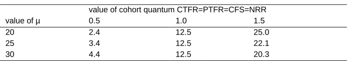
Table 1. Value of period quantum (crude birth rate, per 1000) in stable population

value of cohort quantum CTFR=PTFR=CFS=NRR

value of µ 0.5 1.0 1.5

20 2.4 12.5 25.0

25 3.4 12.5 22.1

30 4.4 12.5 20.3

From the middle column in table 1, we see that the timing of fertility does not affect period quantum in the case of a stationary population, i.e. with cohort fertility exactly at replacement level. In all other situations, timing (tempo) does affect period quantum given cohort quantum, but the direction in which it does so depends on whether cohort fertility is below or above replacement level. In a high fertility situation, period quantum is highest when childbearing occurs at low ages; conversely, in a low fertility situation, period quantum is highest when childbearing occurs at high ages. These relationships are of course pretty trivial, but they are nevertheless useful to illustrate that cohort and period quantum are really different things.

3. Approaches to infer cohort TFR from period TFR

3.1. Period TFR

These two counter points are really two sides of one and the same coin: if we calculate a PTFR as we demographers do routinely, what exactly is it that we are aiming to measure? In fact, what does a PTFR stand for? (Note 1) A PTFR gives us the total number of children a woman will have over her lifetime if:

1. she does not die before menopause;

2. she bears children according to the ASFRs observed during the period in question.

I will not be too harsh about (1). We know that some mortality (Note 2) occurs between birth and age 50, but it is quite limited and quite constant in modern societies. A simple correction for this is sufficient (like having 2.1 instead of 2.0 as benchmark for replacement fertility).

But why would we be interested in measuring (2)? I can see two reasons only: (1) to get an indication about the number of births today. Then why not count these births directly? (2) to get an indication about the extent to which a ‘typical’ woman reproduces herself (Note 3). Then why not calculate cohort TFRs? After all, the typical woman crosses the Lexis diagram diagonally, not vertically.

The inherent problem in calculating cohort TFRs, or other indicators for cohort fertility, is that one is never certain until after the end of the cohort’s reproductive period (i.e. menopause, around age 50). We would so much like to measure, say, how many more children will be born by women currently aged 30, or 35. Basically, we don’t know this: we will just have to wait and see. But we do know quite a lot about fertility above age 30, or age 35, from the experience of previous cohorts, as reflected in recent and current ASFRs. It is so tempting to try and use this information to make statements about the future.

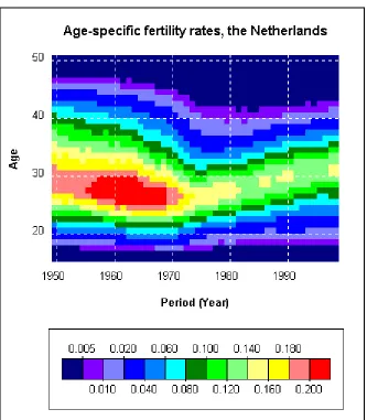
Think of the problem in the following way. We have a Lexis surface of fertility indicators, e.g. ASFRs, or number of births, or ASFRs by birth order, or true age- and parity-specific occurrence-exposure rates. Like the one depicted in figure 1, containing ASFRs for the Netherlands, 1950-1999. Each observation in this Lexis surface belongs to a period (vertical section) and to a cohort (diagonal section). If we want to calculate a summary statistic for a period, we do it vertically, and if for a cohort, diagonally. However, for ‘recent’ cohorts, the observations are censored: we miss those parts of the diagonal section that lie in the future. In principle, we do not know what lies ahead. Nothing has changed here since Ryder (1964, p. 79) wrote: “No cohort parameter can be computed accurately until that cohort has completed the activity being studied”.

Figure 1. ASFRs 1950-1999, the Netherlands (all births)

3.2. Approach 1: demographic translation

One important branch of moving between vertical and diagonal sections of the Lexis surface is known as demographic translation theory (summarized by Keilman 1999). Essentially, translation theory investigates the mathematical relationships between time series of vertical and diagonal summary statistics (Ryder 1964: “expressing the relationship between a time series of cohort indices and a time series of period indices”). For example, in a surface of ASFRs, the column totals give a time series of period TFRs (PTFRs), and the diagonal totals a time series of cohort TFRs (CTFRs). If we knew how PTFRs were related to CTFRs, then we could use up-to-date PTFR values to extrapolate the censored CTFRs. The problem is, though, that the general relationship involves the full Lexis surface, which is censored at today. If the summary statistics develop over time in a particularly smooth fashion, the translation formulas are relatively simple, and censored cohort indicators can be extrapolated with reasonable confidence. For example, the famous translation formula of Ryder (1964) (see also the Appendix):

PTFR=CTFR*(1-DCMAC)

where CMAC is the cohort mean age at child-bearing, holds under the conditions of constant cohort quantum and age-specific proportions in total fertility changing linearly over successive cohorts. However, in practice such smooth conditions are not satisfied. So translation expressions are very useful for theory, and for explaining the past, but for projection purposes they are useful only to the extent that the assumed smooth path will actually continue.

3.3. Approach 2: period adjustment

level of completed fertility implied by current childbearing behavior”. But if such ‘completed fertility’ does not refer to actual cohorts of women, then what does it refer to? Smallwood et al. (2000) are, in my mind, quite correct in stating that “all the[se] adjustments take period data and treat it as if it were a synthetic cohort”. Similarly, Zeng and Land (2000) use the term “hypothetical cohort” in their re-interpretation of the B-F method. Even Bongaarts himself, assuming the UN rapporteur to be correct, is apparently sometimes thinking in cohort terms: “Mr. Bongaarts responded that he was finding the adjusted TFR to be an accurate predictor of cohort fertility” (UN 2000, p. 5). In fact, what the period adjustment approach does is to somehow transform a vertical section into an adjusted vertical section and treat this as if it were a quasi-diagonal section of some sort. I cannot improve on Smallwood’s (2000) formulation: “Tempo adjusted fertility measures provide a way of making a synthetic measure even more synthetic”.

In a nutshell, the B-F method works as follows. Starting point are the period ASFRs, distinguished by birth order. For each period, the sum of these gives PTFRs by birth order, and the age pattern of the ASFRs gives the mean age at child-bearing by birth order (MAC). Over time, the order-specific MACs change. Then B-F calculate SCTFRi=PTFRi/(1-DMACi)) and SCTFR=SSCTFRi, where i denotes birth order and SCTFR is short-hand for synthetic cohort TFR, although B-F do not use this term and call it adjusted TFR instead. The interpretation of this SCTFR is: the TFR that would have been observed in year t if the age pattern of fertility (for each birth order) had been the same as in year t-1, under the assumption that the shape (although not the location) of the order-specific age pattern of the ASFRs is equal in both years.

Is this a useful thing to know? Well, in a way it is. If the constant shape assumption is correct, B-F adjustment shows to what extent timing changes in childbearing can explain changes over time in observed PTFRs in the past (cf. Lesthaeghe and Willems 1999). However, it gives no indication at all on cohort fertility, unless we have some clue as to how close the synthetic cohorts are to real cohorts. If the constant shape assumption is not correct, we have a real problem, because we are even more in the dark as to what the B-F adjusted TFR implies for real cohorts. Elsewhere (Van Imhoff and Keilman 1999; 2000) we have shown that, at least in the Netherlands and Norway, the constant shape assumption is violated by the data.

CTFRs were to move more or less in tandem, this would be really useful knowledge. However, they do not move in tandem, as shown in e.g. Van Imhoff and Keilman (2000) and Smallwood et al. (2000). The SCTFR time series is only slightly closer to the CTFR time series than the PTFR series is; both SCTFR and PTFR display a sharp decline around the end of the baby boom, when fertility tempo changed from advancement to postponement, while the true CTFR shows a much smoother time path.

So my basic empirical objection against these adjusted period measures, i.e. the SCTFR, is that they do not move in tandem with whatever reasonable concept of ‘underlying completed fertility’. In addition, there are two theoretical problems with the SCTFR, both elaborated in Van Imhoff and Keilman (2000).

First, individuals behave conditionally on what they experienced in the past. As a consequence, period effects with an impact on fertility will almost by definition affect different cohorts, each carrying a different past, in a different way. For example, the introduction of the pill obviously had a major impact on fertility behaviour, but the resulting postponement of subsequent births will have been quite different for women who were at the time young and at the start of their fertility career, on the one hand, than for women aged 30+ who already had completed a large portion of their families, on the other hand. So in general, this is a strong theoretical argument against constant period shape.

Second, both B-F and K-P work in terms of age- and parity-specific period fertility rates which express live births by birth order to women irrespective of parity. Thus, the ASFRs are birth frequencies, rather than true occurrence-exposure rates. This presents a problem when adjusting for tempo changes, because the shift in tempo not only affects the numerator but also the denominator of the ratio. As a result, B-F and K-P adjustment applied to frequencies suffers from larger year-to-year fluctuations and therefore gives less reliable insight in the underlying cohort behaviour: the distortion is larger, therefore the adjustment needed is larger, and thus deviations from ‘ideal’ conditions produce wider fluctuations in the time series of the adjusted period measure.

To explain this mechanism, consider first births. These occur to childless women, i.e. women of parity zero. The age-specific pattern of having first births can be described in two ways: via ASFRs, i.e. frequencies, relating first births to all women in that age group; and via o-e rates OE1, relating first births to childless women only. In a cohort, these age-specific measures can be aggregated into one single quantum measure for first births (which is the complement of the quantum measure for permanent childlessness): TFR1 = SASFR1 or F1 = 1-exp(-SOE1). Within a cohort, these two measures yield exactly the same value.

If subsequent cohorts delay the birth of the first child, two things happen. First, the absolute numbers of first births get smaller, for all ages. This depresses the period

proportion of those women really at risk of having first births within the total number of women also changes. As a result, the period TFR1 value is subject to an additional distortion. Women now aged 25 have less first children than women aged 25 last year; as a result, next year there will be more childless women aged 26 then there are now, and as a result today’s ASFR1 age 26 underestimates next year’s ASFR1 for women currently aged 25.

All this does not imply that B-F or K-P applied to frequencies produces systematically biased estimates of synthetic cohort measures. Under ‘ideal’ conditions, in which all cohorts or periods have had the same quantum and same shape and same linear shift over many years, the various adjustments exactly reproduce the underlying cohort measure. Real life will not even come close to this ideal situation. In real life, it matters whether one adjusts period measures based on frequencies or based on o-e rates, the latter being more robust than the former. I should also add that the ‘constant period shape’ assumption underlying the B-F and K-P adjustments can be applied to the age pattern of the frequencies or to the age pattern of the o-e rates, but generally not to both at the same time (except under ‘ideal’ circumstances).

3.4. Approach 3: period extrapolation to complete censored cohorts

In a series of recent papers, Kohler and Ortega (2001a, 2001b) have developed an approach which initially looks like just a refinement of the K-P period adjustment, but is in fact fundamentally different. The Kohler-Ortega (K-O) approach differs from K-P in three important aspects:

1. O work in terms of age- and parity-specific occurrence-exposure rates, while K-P work in terms of age- and parity-specific fertility rates (frequencies). As we saw earlier, o-e rates are less sensitive to tempo changes than frequencies.

2. K-O make statements about real cohorts, while K-P work in terms of synthetic

cohorts (or, equivalently, ‘an adjusted period index interpreted as some cohort index’). K-O do this by taking each cohort’s fertility history until now as given, and using the observed period rates only to complete each censored cohort’s fertility career.

Essentially, what the K-O approach does is the following. For each birth order, the starting point is the Lexis surface of o-e rates. A study is made of the way in which the vertical sections of this Lexis surface, i.e. the period age patterns of o-e rates, change over time. Subsequently, a choice is made as to how this information should be used to extrapolate the most recently observed period age pattern into the future. Finally, these extrapolations of the period age pattern are used to complete the cohort o-e age schedules, and make various statements about completed fertility of successive cohorts (including its breakdown by birth order).

All cohorts’ fertility careers are known up to and including the most recent (‘current’) period. What is going to happen in the future depends on the assumption made concerning the continuation of recent changes in period age patterns. Here, K-O investigate three alternatives:

1. ‘Observed’: the currently observed period o-e rates are kept constant throughout. Naturally, this is not a realistic assumption, because (as K-O also stress) the period schedule is distorted by tempo changes and therefore does not reflect a true cohort experience. Under conditions of fertility postponement, the ultimate proportion of mothers under ‘observed’ will (potentially seriously) underestimate the true CCF1.

2. ‘Postponement stops’: the currently observed period o-e rates are adjusted for tempo changes (using the K-P method, i.e. constant period shape but taking into account recent changes in period mean and variance) and kept constant throughout. This will give an accurate estimate of the true CCF1, provided that the adjusted current period shape is an accurate reflection of the remaining cohort fertility career. I will return to this issue below.

I consider the K-O projections as a major improvement over the B-F and K-P adjusted period TFRs, precisely for the three reasons listed above: o-e rates are less distorted indicators than ASFRs; K-O work in terms of real cohorts; and K-O are explicit on the assumptions underlying their completion of censored cohorts (cf. Lesthaeghe and Willems 1999; Lesthaeghe 2001).

However, there are still some problems left. The first problem has to do with the fertility ageing effect. It is quite likely that such an effect exists, if only for biological and medical reasons: the older women (or men!) are when they start trying to have children, the higher the probability that they will be disappointed. So total fertility will probably fall somewhat as the mean age increases. However, this mechanism is quite different from how it works under K-O: there, total fertility falls because the o-e schedule for a given birth order shifts to the right at a faster pace than the o-e schedule for the next birth order. This seems quite unlikely from a perspective of an individual woman: if she decides to postpone her family formation, all o-e schedules will be shifted right in tandem, not at different paces. In fact, K-O explicitly assume that o-e rates are independent of the timing of previous births; I do not find this assumption very realistic.

The second problem was already referred to above: cohorts’ o-e schedules are completed on the basis of the current period o-e schedule (possibly after some period-inspired adjustments). I do not see a good theoretical reason why period shapes must be representative for cohort shapes. In terms of o-e rates, the procedure to use period shapes for cohorts is by all means more justifiable than in terms of ASFRs, but exactly how justifiable can only be verified empirically: by comparing K-O projected cohort fertility with actual cohort fertility.

The third problem is essentially the same as with B-F and K-P, namely that the adjustment of the current period o-e rates is based on recent changes in period shape, with no (B-F: constant shape) or limited (K-P: variance changes) period-cohort interaction. Since individuals behave conditionally on what they experienced in the past, period effects with an impact on fertility will almost by definition affect different cohorts, each carrying a different past, in a different way.

crossing the Lexis surface horizontally, which are due to differences between subsequent cohorts and therefore not relevant for individual cohorts. Therefore, I think that the ‘postponement stops’ scenario is by far the most likely K-O projection of

cohort fertility.

3.5. Conclusion for cohort quantum

My conclusion from all this is the same as Ryder reached back in 1964, already quoted above: “No cohort parameter can be computed accurately until that cohort has completed the activity being studied”. Any procedure trying to estimate cohort quantum from period quantum is based on simplifying assumptions, the justifiability of which can only be verified empirically: by comparing the estimated cohort fertility with actual cohort fertility.

This conclusion not only applies to explaining what happened to periods and cohorts in the past, but even more so to fertility forecasting. Lesthaeghe (2001) very convincingly shows that it is essential to study explicitly the postponement and recuperation behaviour of successive cohorts when forecasting into the future: “… techniques applied to period data can be abandoned for national forecasts in favour of cohort-based approaches. …. forecasts based on period measures …. totally ignore the intricacies of cohort behaviour with respect to postponement and recuperation” (p. 27).

So we definitely must study cohort quantum directly, which is what I will do in the next section for two countries: the Netherlands and Italy.

4. An empirical analysis of cohort fertility trends in the Netherlands

and Italy

4.1. Data

Statistics Netherlands (SN) has a complete set of data on births by age (14+) and birth order from 1950 onwards only. Thus, order-specific ASFRs can be calculated for periods 1950-present and for cohorts 1936 and later. All data are of the period-cohort type (Lexis parallelograms): birth are classified by the age of the mother as per 31 December, i.e. by the difference between calendar year of the birth and the birth year of the mother.

population is missing. What SN does instead, and I have done this as well, is to reconstruct the parity distribution from historical ASFRs by birth order. The problem for historical data is that before 1967 municipalities were not required by law to register parity: some did, some did not. Thus, today the population register contains 100% reliable information on parity for women born since 1967 only. There remain some problems, e.g. regarding the statistical treatment of adopted children and multiple births, but these are minor. From Statistics Netherlands I have received the observed parity distribution for 1 January 2000. There are some oddities, but on the whole the observed 1 January 2000 distribution is almost indistinguishable from the reconstructed 31 December 1999 distribution.

This close correspondence between reconstructed and observed parity distribution also implies that historical ASFRs can safely be used to reconstruct the fertility career of cohorts. Theoretically, it is possible that substantial migration flows, together with migrants having widely different parity distributions from non-migrants, cause cohort distributions to become different from cumulative ASFRs. However, from the close correspondence for 2000, it follows that this theoretical possibility can be safely ignored in practice.

For Italy, I have obtained, by kind permission of ISTAT, a similar dataset, containing total female population by age (13+) and births by age and birth order for the years 1952..1996. Thus, order-specific ASFRs can be calculated for periods 1952-present and for cohorts 1939 and later. All data are of the period-age type (Lexis squares): births are classified by the age of the mother at the time of birth.

4.2. Period trends and B-F adjustment

Figure 2 plots the observed and B-F adjusted period TFR for the Netherlands and Italy. During the ‘baby boom’ period, the adjusted TFR lies below the observed TFR, and during the ‘baby bust’ period it is the other way round. This reflects the fact that the ‘baby boom’ period was one of accelerating tempo, and the ‘baby bust’ period one of delayed tempo. From the curves for MAC1 (mean age at childbearing for first births), it can be seen that the turning point in the Netherlands occurred around 1970, and in Italy around 1975.

The big question is what these unadjusted and adjusted period measures tell us about the underlying cohort quantum of fertility.

figure 2 we see immediately that this is not the case. For the B-F adjusted TFR, the condition is the constant shape assumption: “women of all ages bearing children [of a given birth order] in year t defer or advance their births to the same extent, independently of their age or cohort identification” (Bongaarts and Feeney, 1998, p. 277). Formally, this assumption amounts to stating that the expression

)

(

]

),

(

[

)

(

t

TFR

t

t

MAC

x

ASFR

x

z

i i i

i

−

=

Figure 2. Observed and B-F adjusted TFR, Netherlands and Italy

Source: Statistics Netherlands.

Source: ISTAT.

Netherlands

1.00 1.50 2.00 2.50 3.00 3.50

1950 1955 1960 1965 1970 1975 1980 1985 1990 1995 2000 24 25 26 27 28 29

ObsTFR AdjTFR MAC1

Italy

1.00 1.50 2.00 2.50 3.00 3.50

1950 1955 1960 1965 1970 1975 1980 1985 1990 1995 2000 24 25 26 27 28 29

Figure 3a. Distance from MAC1 at given cumulative percentages of fertility schedule, first births, Netherlands

Figure 3b. Distance from MAC1 at given cumulative percentages of fertility schedule, first births, Italy

4.3. Looking at cohort quantum directly

Another way of looking at this is, to study cohort quantum directly, and see how close B-F adjustment (or K-P, or K-O) brings us to this true cohort quantum. The inherent problem here, again, is that for recent cohorts we do not know what their ultimate quantum will be, so we will have to do some extrapolation.

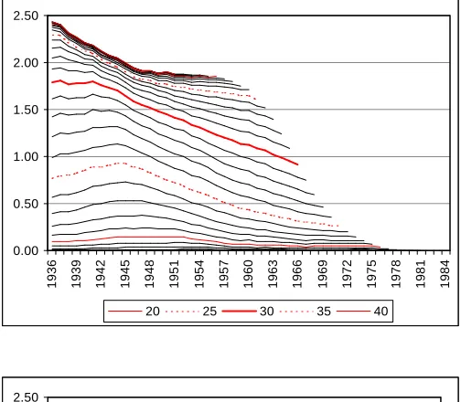
Figure 4a: Average number of children, by age and cohort, Netherlands

Source: Statistics Netherlands.

0.00 0.50 1.00 1.50 2.00 2.50

1936 1939 1942 1945 1948 1951 1954 1957 1960 1963 1966 1969 1972 1975 1978 1981 1984

20 25 30 35 40

0.00 0.50 1.00 1.50 2.00 2.50

15 20 25 30 35 40 45

Figure 4b: Average number of children, by age and cohort, Italy

Source: ISTAT.

0.00 0.50 1.00 1.50 2.00 2.50

1936 1939 1942 1945 1948 1951 1954 1957 1960 1963 1966 1969 1972 1975 1978 1981 1984

20 25 30 35 40

0.00 0.50 1.00 1.50 2.00 2.50

15 20 25 30 35 40 45

First look at the upper graph for the Netherlands. Dutch fertility accelerates between cohorts 1936 and 1945, followed by an abrupt and quite fast postponement for women born after 1945. Only for the most recent cohorts are there some signs that the postponement of births might be coming to an end. At the same time, the CTFR falls steadily from 2.40 for cohort 1936 to about 1.80 for cohort 1950, and remains more or less constant thereafter. If something like a ‘fertility ageing effect’ exists, it certainly does not show up in this graph for the Netherlands. On the contrary: acceleration and

falling completed family size go hand in hand, while postponement seems to have very little, if not zero, effect on ultimate fertility in the Netherlands.

The lower graph shows the same trends in a different manner. This graph starts with cohort 1950, so it only describes the postponement part of the recent fertility history. Subsequent cohorts shift their cumulative childbearing pattern to the right (but note that 1975 is very close to 1970, suggesting that the end of postponement might be near), but they all end up, or appear to be going to end up, at pretty much the same level, around or possibly slightly below 1.80. So although Dutch cohorts drop behind their predecessors at younger ages to quite a large extent, they recuperate almost all of this at higher ages.

In Italy, the acceleration phase ended about five years later than in the Netherlands, until about cohort 1950; the pace of the acceleration is somewhat weaker than in the Netherlands. Then, postponement started, first slowly, but later on more convincingly. By the end of the observation period, i.e. 1996, there are as yet hardly any signs of postponement coming to an end in Italy. Completed fertility fell from 2.20 for cohort 1939 to about 1.80 for cohort 1950. However, contrary to the Netherlands, it is hard to tell whether a fertility ageing effect is occurring in Italy. The curves suggest that recuperation at higher ages is much weaker than in the Netherlands, which implies that the postponement in Italy is going to be associated with smaller completed family size.

The lower graph for Italy tells more or less the same story. Cohort 1960 has dropped so far behind cohort 1955 that it seems unlikely that it will end up at the 1.80 CFS of cohort 1955. In its turn, cohort 1965 seems unlikely to fully overtake cohort 1960. So for the more recent cohorts in Italy, the ultimate value of the CTFR might well be somewhat below 1.80, although the extent to which it will fall short of 1.80 is difficult to tell.

stay there for even more recent cohorts. In Italy, the 60% remained at age 25 until about cohort 1955, after which an even faster decline occurred than in the Netherlands, reaching 25% for cohort 1970 with no signs yet of a stabilization.

Figure 5a: Percentage women with at least one child, by age and cohort, Netherlands

Source: Statistics Netherlands. 0.00 0.10 0.20 0.30 0.40 0.50 0.60 0.70 0.80 0.90 1.00

1936 1939 1942 1945 1948 1951 1954 1957 1960 1963 1966 1969 1972 1975 1978 1981 1984

20 25 30 35 40

0.00 0.10 0.20 0.30 0.40 0.50 0.60 0.70 0.80 0.90 1.00

15 20 25 30 35 40 45

Figure 5b: Percentage women with at least one child, by age and cohort, Italy

Source: ISTAT.

0.00 0.10 0.20 0.30 0.40 0.50 0.60 0.70 0.80 0.90 1.00

1936 1939 1942 1945 1948 1951 1954 1957 1960 1963 1966 1969 1972 1975 1978 1981 1984

20 25 30 35 40

0.00 0.10 0.20 0.30 0.40 0.50 0.60 0.70 0.80 0.90 1.00

15 20 25 30 35 40 45

For the Netherlands, we see CTFR1 falling slightly from 0.90 for older cohorts to 0.80 for cohorts 1960 and younger. From the lower graph, too, the substantial postponement of first births at younger ages is almost fully compensated by recuperation at older ages. In Italy, the decline from the initial 0.90 has started more recently, and it is hard to tell where it will end up. Graphically extrapolating the censored cohorts in the lower graph, an ultimate value of 0.80 or perhaps 0.75 for cohort 1970 seems not unreasonable (the Italian 1970 cohort is more or less on the same track as cohort 1965 in the Netherlands).

For second children (figure 6), there is some evidence in the Netherlands for a ‘fertility ageing effect’: although CTFR2 did not increase during the acceleration phase, it did decrease a little during the first years of the postponement phase, from about 0.75 for cohort 1945 to slightly below 0.70 for cohorts 1955 and later. Here too, the most recent cohorts show signs of stabilizing tempo. The CTFR2 might end up at 0.65 or so. In Italy, the fall in the CTFR2 starting after cohort 1945 has been somewhat stronger, and it might continue some more. Because the postponement process is still very much going on, it is difficult to extrapolate the censored cohorts in the lower graph. 0.60 or 0.55 looks not too bad.

The trend in third children (figure 7) for both countries appears to be unrelated to tempo changes. In the Netherlands, CTFR3 falls from 0.45 for cohort 1936 to between 0.20 and 0.25 for cohorts 1945 and younger. For cohorts born in the late 1950s, third children are slightly more common than for cohorts born around 1950; it is not immediately clear what has caused this slight (temporary) ‘revival’ of larger family sizes, although it could have something to do with family reunification migration in the late 1970s and early 1980s. In Italy, the falling trend in CTFR3 has not yet come to an end: cohort 1960 will have to recuperate quite a lot to finish at 0.20 and for younger cohorts 0.15 seems a more likely ultimate value.

Finally, families with four children or more (figure 8) have become quite rare indeed. As for third children, this falling trend seems to be associated with a ‘real’ desire for smaller families and not with changes in tempo. In the Netherlands, CTFR4 has declines very sharply from 33% for cohort 1936 to around 10% for cohort 1945 and later. Recently (cf. cohort 1965 in the lower graph), fourth births have started to be postponed again, which makes it somewhat unlikely that CTFR4 will remain at 0.10 for the most recent cohorts; 0.05 seems a safe lower limit. In Italy, we see an almost equally strong decline in CTFR4, which shows as yet no sign of levelling off. An ultimate level of 0.05 seems a fair guess.

Figure 6a: Percentage women with at least two children, by age and cohort, Netherlands

Source: Statistics Netherlands. 0.00 0.10 0.20 0.30 0.40 0.50 0.60 0.70 0.80

1936 1939 1942 1945 1948 1951 1954 1957 1960 1963 1966 1969 1972 1975 1978 1981 1984

20 25 30 35 40

0.00 0.10 0.20 0.30 0.40 0.50 0.60 0.70 0.80

15 20 25 30 35 40 45

Figure 6b: Percentage women with at least two children, by age and cohort, Italy

Source: ISTAT.

0.00 0.10 0.20 0.30 0.40 0.50 0.60 0.70 0.80

1936 1939 1942 1945 1948 1951 1954 1957 1960 1963 1966 1969 1972 1975 1978 1981 1984

20 25 30 35 40

0.00 0.10 0.20 0.30 0.40 0.50 0.60 0.70 0.80

15 20 25 30 35 40 45

Figure 7a: Percentage women with at least three children, by age and cohort, Netherlands

Source: Statistics Netherlands. 0.00 0.10 0.20 0.30 0.40 0.50

1936 1939 1942 1945 1948 1951 1954 1957 1960 1963 1966 1969 1972 1975 1978 1981 1984

20 25 30 35 40

0.00 0.10 0.20 0.30 0.40 0.50

15 20 25 30 35 40 45

Figure 7b: Percentage women with at least three children, by age and cohort, Italy

Source: ISTAT.

0.00 0.10 0.20 0.30 0.40 0.50

1936 1939 1942 1945 1948 1951 1954 1957 1960 1963 1966 1969 1972 1975 1978 1981 1984

20 25 30 35 40

0.00 0.10 0.20 0.30 0.40 0.50

15 20 25 30 35 40 45

Figure 8a: Percentage women with four or more children, by age and cohort, Netherlands

Source: Statistics Netherlands. 0.00 0.10 0.20 0.30 0.40

1936 1939 1942 1945 1948 1951 1954 1957 1960 1963 1966 1969 1972 1975 1978 1981 1984

20 25 30 35 40

0.00 0.10 0.20 0.30 0.40

15 20 25 30 35 40 45

Figure 8b: Percentage women with four or more children, by age and cohort, Italy

Source: ISTAT.

0.00 0.10 0.20 0.30 0.40

1936 1939 1942 1945 1948 1951 1954 1957 1960 1963 1966 1969 1972 1975 1978 1981 1984

20 25 30 35 40

0.00 0.10 0.20 0.30 0.40

15 20 25 30 35 40 45

Table 2: Estimated cohort fertility for recent cohorts, Netherlands and Italy

Netherlands Italy

Completed fertility for cohorts born around 1970 and later

Birth order 1 0.80 0.75-0.80

Birth order 2 0.65-0.70 0.55-0.60

Birth order 3 0.20 0.15-0.20

Birth order 4 0.05-0.10 0.05

Total completed family size 1.70-1.80 1.50-1.65

Period TFR 1990s 1.50-1.65 1.20-1.35

B-F adjusted TFR 1990s 1.70-1.95 1.50-1.70

The CTFRs in table 2 are not based on any sophisticated models or theoretical arguments. They are educated guesses, based on the fertility experiences of successive cohorts, and graphically inspired recuperation assumptions. For the Netherlands, I feel more confident about these assumptions than for Italy. The reasons for this relative confidence are twofold: first, they are shared by the demographic analysts at Statistics Netherlands (and indeed, my assumptions are the same as those underlying the 2000 SN population forecast); second, the graphical trends are fairly stable in the Netherlands. In contrast, the Italian cohort experience is more difficult to predict, because Italian women are still very much in the middle of drastically reorganizing their fertility careers. We know for sure that fertility at younger ages is falling in Italy: what we do not know is the answer to the decisive question whether this fall in low-age fertility is merely postponement, or rather a structural shift towards really smaller families. We simply don’t know where Italian fertility is heading to: we just have to wait and see.

What is clear from the table is that period fertility indicators are distorted: with these drastic tempo changes going on, period TFRs are grossly underestimating the reproductive behaviour of real women, i.e. cohorts. The B-F adjusted TFR succeeds at least in providing the “improved reading of period fertility” it was designed for (Bongaarts and Feeney 1998, p. 289). For the period considered, i.e. the 1990s, this improved reading is more successful for Italy than for the Netherlands, because the tempo changes in Italy are more pervasive, in all respects going in the same direction; as a result, the constant shape assumption underlying the B-F procedure is better satisfied in Italy than in the Netherlands.

continues’). On the other hand, based on reference year 1998 K-O obtain ultimate CTFR values of around 1.60 for all three scenarios, which appears to be too low when compared to the trends for real cohorts depicted in figures 4-8.

5. Conclusions

Period and cohort quantum indicators (of fertility or whatever) are two fundamentally different concepts. If we are interested in a period perspective, e.g. to assess the future of our educational system or our pension scheme, we must look at annual births directly (either in absolute or in relative CBR terms). If we are interested in a cohort perspective, e.g. to assess the extent to which generations replace themselves, then we must look at cohort fertility directly.

I have critically reviewed several existing attempts to infer cohort fertility from period fertility measures. Whether such attempts are successful essentially depends on whether the assumptions underlying the method are satisfied: if they are, it is; if they are not, it isn’t. In general, there is no reason why a method’s underlying assumptions should be satisfied. They might be all right, but the only way of finding out is to look at the data directly. And once we do that, we do not need the adjustment method any more, because we are looking at the cohort data we were interested in in the first place.

In the practice of European countries passing through the various stages of the Second Demographic Transition, quantum and tempo effects from a period and cohort perspective are interwoven in a subtle and complex way. As a result, a single measure can never produce the full story. Graphical tools to access large amounts of information, demographic insight and common sense still do a better job than synthetic measures.

6. Acknowledgements

Notes

1. The text that follows criticizes the beharioural interpretation that can be attached to a period TFR. This criticism does not imply that the PTFR is altogether useless, as a synthetic indicator of fertility. In particular, for comparative research (either between regions or countries, or over time), the PTFR has as a major advantage that, unlike the CBR, it is not sensitive to the age composition of the female population of child-bearing age.

2. Apart from mortality, the distortionary effect of which is limited, migration is potentially a more important factor that should be kept in mind when calculating TFRs. The smaller the region to which the TFR applies, the larger the scope for distortionary migration effects. Examples include: couples moving out of inner cities before starting families; women living in regions without a hospital give birth in a neighbouring region; international marriage migration.

References

Bongaarts J., Feeney G. (1998). “On the quantum and tempo of fertility.” Population and Development Review, 24, 2: 271-291.

Keilman N. (1999). Demographic translation: from period to cohort perspective and back. In: Caselli G., Vallin J., Wunsch G., editors. Demographie: analyse et synthèse. Actes du Séminaire de Roma, Napoli, Puzzuoli. Volume 2. Paris: INED, 1-14.

Kohler H.P., Ortega J.A. (2001a). Period parity progression measures with continued fertility postponement: A new look at the implications of delayed childbearing for cohort fertility. Rostock: Max-Planck Institute for Demographic Research. Working Paper 2001-001.

Kohler H.P., Ortega J.A. (2001b). Period parity progression measures with continued fertility postponement: Assessing the implications of delayed childbearing for fertility in Sweden, the Netherlands and Spain. Rostock: Max-Planck Institute for Demographic Research. Manuscript, 16 March 2001.

Kohler H.P., Philipov D. (2001). “Variance effects in the Bongaarts-Feeney formula.”

Demography, 38, 1: 1-16.

Lesthaeghe R. (2001). Postponement and recuperation: Recent fertility trends and forecasts in six Western European countries. IPD-WP 2001-1. Brussel: Vrije Universiteit. Paper presented at the IUSSP Seminar on “International Perspectives on Low Fertility: Trends, Theories and Policies”, Tokyo, 21-23 March 2001.

Lesthaeghe R., Willems P. (1999). “Is low fertility a temporary phenomenon in the European Union?” Population and Development Review, 25, 1: 211-228.

Rallu J.L., Toulemon L. (1994). “Period fertility measures: The construction of different indices and their application to France, 1946-89.” Population: An English Selection, 6: 59-94.

Ryder N.B. (1964). “The process of demographic translation.” Demography, 1, 1: 74-82.

Smallwood S. (2000). A comparison of four tempo adjusted fertility measures applied to England and Wales data, 1940-1997. London: London School of Economics. Unpublished MSc dissertation.

UN (2000), Below replacement fertility. Population Bulletin of the United Nations, Special Issue 40/41 1999. New York: United Nations.

Van Imhoff E. and Keilman N. (1999). On the quantum and tempo of fertility: comment. The Hague: NIDI. Working Paper 1999/2. http://www.nidi.nl/public/nidi_wp_1999_2.pdf

Van Imhoff E., Keilman N. (2000). “On the quantum and tempo of fertility: comment.”

Population and Development Review, 26, 3: 549-553.

Yntema L. (1977). Inleiding tot de demometrie. Deventer: Van Loghum Slaterus.

Appendix

The general translation equation is due to Ryder (1964). Here we present it in the notation of Keilman (1999).

Notation

m(t,x) is the age-specific (fertility) rate (age x, period t)

A(t) is period quantum (PTFR):

=

∑

x

x

t

m

t

A

(

)

(

,

)

B(g)=B(t-x) is cohort quantum (CTFR):

=

∑

+

x

x

x

g

m

t

B

(

)

(

,

)

b(g,x)=m(g+x,x)/B(g) is the age schedule (of fertility) for cohort g.

∑

=

x

k

k

g

x

b

g

x

M

(

)

(

,

)

is the k’th (absolute) moment of the cohort age schedule.

∑

=

x i k i

k

g

x

b

g

x

M

()

(

)

()

(

,

)

is the i’th derivative of the k’th absolute moment, where

derivatives are understood to be with respect to t and g, not x.

We now have (using Taylor series expansion):

=

−

×

−

=

∑

x

x

x

t

b

x

t

B

t

A

(

)

(

)

(

,

)

∑

=     − + − ×     − + − = x x t b x x t xb x t b t B x t xB t B ... ! 2 ) , ( ) , ( ) , ( ... ! 2 ) ( ) ( ) ( ) 2 ( 2 ) 1 ( ) 2 ( 2 ) 1 (

∑

∑

= = − −

















−

−

−

=

0 ) ( ) ( ) (

)!

(

)

(

)

1

(

!

)

(

)

1

(

i j i

i j j i j i i

i

j

t

M

i

t

B

Ryder’s special case for linear tempo shift

Now suppose cohort quantum B is constant; all its derivatives vanish. In addition, suppose the age-specific proportions b(g,x) develop linearly over time g; then the first derivative of all moments is constant, and all second and higher-order derivatives of the moments vanish. The equation then reduces to:

)

1

(

)

(

t

A

B

M

₁(1)

A

=

=

×

−

Now

M

₁ is the cohort’s mean age, and

M

₁(1) is the annual change in this cohort mean age. Thus, the translation equation says: under constant cohort quantum and linear age-specific proportions, period quantum falls short of cohort quantum by a fraction equal to the annual change in the cohort mean age. If we denote this annual change in cohort mean age by r, the original Ryder translation equation is

)

1

(

r

B

A

=

×

−

However, this is not the same as a constant linear shift of the cohort age schedule. If, say, a bell-shaped curve moves linearly to the right, each age-specific proportion will change from year to year according to the form of the bell and the speed of the shift, and this change will certainly not be linear over time.

Also, the conditions spelled out for the above result are not necessarily equivalent to a linear change in the cohort mean age, as Keilman (1999) seems to suggest. Linear age-specific proportions imply linear cohort mean age, but the reverse is not true. For example, a linear shift of the cohort age schedule does imply linear cohort mean age but not linear age-specific proportions.

Direct derivation

So what does the translation equation look like under a linear shift of the cohort age schedule and constant cohort quantum? Suppose the schedule shifts to the right by r

years per calendar year; r is then also the annual change in the cohort mean age. A constant annual shift by r years implies:

Now we have:

r

B

dy

y

t

b

r

B

dx

xr

x

t

b

B

dx

x

x

t

b

B

A

t

A

+

=

+

=

+

=

−

×

=

=

_∫

∞

_∫

∞

_∫

∞

1

)

,

(

1

)

,

(

)

,

(

)

(

0 0 0

So instead of multiplying by (1-r), we should divide by (1+r). This I call the ‘modified’ Ryder translation equation.

The cohort mean age changes linearly over time. It equals:

∫

∞

×

=

0

)

,

(

)

(

g

x

b

g

x

dx

CMAC

for cohort born in year g. For the period mean age,

we have:

r

t

CMAC

r

dy

y

t

b

r

dy

y

t

b

y

dx

xr

x

t

b

dx

xr

x

t

b

x

dx

x

x

t

b

dx

x

x

t

b

x

t

PMAC

+

=

+

+

×

=

+

+

×

=

−

−

×

=

∫

∫

∫

∫

∫

∫

∞ ∞ ∞ ∞ ∞ ∞

1

)

(

)

1

(

)

,

(

)

1

(

)

,

(

)

,

(

)

,

(

)

,

(

)

,

(

)

(

0 2 0 0 0 0 0

So the ratio of period mean age and cohort mean age is constant. In particular, when the cohort mean age changes linearly at r per annum, the period mean age changes linearly at r/(1+r) per annum. These changes are therefore not equal.

We now see also that the ‘modified Ryder’ translation equation A=B/(1+r) is equivalent to B-F’s adjustment B=A/(1-q) where q is the annual change in the period

mean age. Namely: A=B*(1-q)=B*(1-r/(1+r))=B/(1+r).

Derivation of ‘modified Ryder’ via general translation formulas

∑

∞ = +

−

=

0 ) (

)

(

!

)

1

(

)

(

i i i k i

k

W

t

i

t

V

∑

∞ = +

=

0 ) (

)

(

!

1

)

(

i i i k

k

V

t

i

t

W

where Vk(t) is the k’th absolute moment for period t, and Wk(t) is the k’th absolute

moment for the cohort born in t.

Normalize the absolute moments as follows:

)

(

/

)

(

)

(

t

V

t

V

0

t

v

k

=

k

)

(

/

)

(

)

(

t

W

t

W

0

t

w

k

=

k

These are the moments of the normalized age schedule (i.e. the normalized age-specific rates add up to 1, as a proper probability function). V0(t) and W0(t) are TFR and

CCF, respectively.

Apply the translation equation first to the 0’th moment:

∑

∑

∞ = ∞ =

−

=

−

=

0 ) ( 0 0 ) (

0

(

)

!

)

1

(

)

(

)

(

!

)

1

(

)

(

i i i i i i i i

t

w

i

t

W

t

W

i

t

V

A normalized absolute moment is a power series involving deviations from the mean and the mean itself, e.g.:

i k x k i i x

k

x

m

m

i

k

p

m

− =

∑ ∑

_



_



−

=

(

)

(

1

)

0

1

Suppose we have constant cohort quantum, constant cohort shape, and an annual linear shift of the cohort age schedule at rc per annum. Then all deviations from the

c c c c c

r

CCF

r

W

r

r

r

W

TFR

V

+

=

+

=

+

−

+

−

=

=

1

1

...)

1

(

2 3 0

0 0

which is equivalent to ‘modified Ryder’.

Now apply the translation equation to the 1’st moment:

∑

∞ = +

−

=

×

=

0 ) ( 1 0 1 0

1

(

)

!

)

1

(

)

(

)

(

)

(

)

(

i i i i

t

w

i

t

W

t

v

t

V

t

V

Suppose again constant cohort quantum, constant cohort shape, and an annual linear shift of the cohort age schedule at rc per annum. Then we have, using the same

reasoning as above:

w

k_k

(

k

1

)!

w

1

(

t

)

(

r

_c

)

k

) (

1+

=

+

×

. Substitution gives:

...)

4

3

2

1

(

)

(

)

(

_{0 1} 2 3

1

0

×

v

t

=

W

×

w

t

×

−

r

c

+

r

c

−

r

c

+

V

from which

=

+

−

+

−

×

+

×

=

+

−

+

−

×

×

=

(

)

(

1

2

3

4

...)

(

)

(

1

)

(

1

2

3

4

...)

)

(

₁ 2 3 ₁ 2 3

0 0

1

w

t

r

c

r

c

r

c

w

t

r

c

r

c

r

c

r

c

V

W

t

v

c c c c

r

t

w

r

r

r

t

w

+

=

+

−

+

−

×

=

1

)

(

...)

1

(

)

(

2 3 1

1

So the period mean age is a distorted version of the cohort mean age. The cohort mean age develops linearly over time, at rc per annum. Then the period mean age will

also be linear, at rp = rc/(1+ rc) per annum.