www.elsevier.com/locate/ic
Buildingsmall equality graphs for decidingequality
logic with Uninterpreted Functions
Yoav Rodeh
a, Ofer Strichman
b ,∗ aTel-Hai College, Tel-Hai, IsraelbInformation Systems Engineering, Technion, Haifa, Israel
Received 19 September 2004; revised 1 June 2005 Available online 13 September 2005
Abstract
The logic of equalities with Uninterpreted Functions is used in the formal verification community mainly for proofs of equivalence: provingthat two versions of a hardware design are the same, or that input and output of a compiler are semantically equivalent are two prominent examples of such proofs. We introduce a new decision procedure for this logic that generalizes two leading decision procedures that were published in the last few years: the Positive Equality approach suggested by Bryant et al. [Exploitingpositive equality in a logic of equality with uninterpreted functions, in: Proc. 11th Intl. Con-ference on Computer Aided Verification (CAV’99), 1999], and the Range-Allocation algorithm suggested by Pnueli et al. [The small model property: how small can it be? Information and Computation 178 (1) (2002) 279–293]. Both of these methods reduce this logic to pure Equality Logic (without Uninterpreted Functions), and then, due to the small model property that such formulas have, find a small domain to each variable that is sufficiently large to maintain the satisfiability of the formula. The state-space spanned by these domains is then traversed with a BDD-based engine. The Positive Equality approach identifies terms that have a certain characteristic in the original formula (before the reduction to pure Equality Logic), and replaces them with unique constants. The Range-Allocation algorithm analyzes the structure of the formula after the reduction to equality logic with a graph-based procedure to allocate a small set of values to each variable. The former, therefore, has an advantage when a large subset of the terms can be replaced with constants, and disadvantage in the other cases. In this paper we es-sentially merge the two methods, while improving both with a more careful analysis of the formula’s
∗Correspondingauthor.
E-mail addresses:[email protected] (O. Strichman), [email protected] (Y. Rodeh). 0890-5401/$ - see front matter © 2005 Elsevier Inc. All rights reserved.
structure. We show that the new method is provably dominant over both methods, theoretically as well as empirically.1
© 2005 Elsevier Inc. All rights reserved.
1. Introduction
The logic of Equalities with Uninterpreted Functions (EUF) has been used rather extensively in the last decade in the formal verification community, and several sophisticated decision procedures for this logic were suggested [12,3,15,4] (see [20] and Appendix A for a survey). Using Uninterpreted Functions rather than the original functions in the verification condition abstracts away information that is not necessarily needed for the proof, and hence simplifies and generalizes the proof. From a given EUF-formulaϕEUF, it is possible to derive an Equality formula (E-formulafrom now on)ϕEthat
is satisfiable if and only if there exists a satisfyinginterpretation toϕEUF. The reduction to Equality
Logic must preserve thefunctional consistencyproperty which is common to all functions, i.e., that they return the same value if instantiated with the same arguments. When functional consistency is all that is necessary for the proof, it simplifies greatly the task of performing it mechanically. It is only left, then, in these cases, to decide a pure E-formula.
Several examples of usage of this logic in the verification community are: proving equivalence between two versions of hardware designs [9,4]; Translation Validation [16], a process in which the correctness of a compiler’s translation is proven by checkingthe equivalence of the source and target codes; and checkinga control property of a microprocessor, where it is sufficient to specify that the operations which the ALU perform are functions, rather than specifyingwhat these operations are (thus avoidingthe complexity of the ALU). This is the approach taken, for example, in [9], where a formula with Uninterpreted Functions is generated, such that its validity implies the equivalence between the two versions of the CPU, with and without a pipeline.
By now there are quite a few decision procedures for equality logic, most of which we cover in Appendix A. Here, we briefly mention two prior works that are directly related to what we suggest:
thePositive Equalityapproach suggested by Bryant et al. [3] which was later extended toRobust
Positive Equalityby Lahiri et al. [13], and theRange-Allocationapproach suggested by Pnueli, Rodeh,
Strichman and Siegel in [15]. Both of these methods are instantiations of the following scheme: (1) ReduceϕEUF to an E-formulaϕEsuch thatϕE is satisfiable if and only if there exists an
inter-pretation which satisfiesϕEUF.
(2) Analyze the formula’s predicates (by examininga graph representation of the formula, as we will later explain) to calculate anadequate domainRfor each variable inϕE, that is, a domain
large enough so that if there exists a satisfying assignment for ϕE, then there exists such an
assignment within this domain.
(3) Check (symbolically) if any of the assignments inRsatisfyϕE.
1An early version of this article appeared in [Y. Rodeh, O. Shtrichman, Finite instantiations in equivalence logic
with uninterpreted functions, in: G. Berry, H. Comon, A. Finkel (Eds.), Proc.13th Intl. Conference on Computer Aided Verification (CAV’01), Lecture Notes in Computer Science, Springer-Verlag, Berlin, 2001.]
In Section 4, we will redefine this scheme more accurately after giving the necessary formal definitions. Our suggested procedure replaces Steps 1 and 2 with one improved step. The main idea is to exploit information which is only visible in the original formulaϕEUFbefore its reduction toϕE.
The Positive Equality approach identifies terms that have a certain syntactical characteristic in the original formula, and replaces them with unique constants. Briefly, these terms need to be compared to one another only under negative polarity and not be used as guards in ITE expressions (see Section 5), in order to be substituted with constants.
The Range-Allocation algorithm, on the other hand, does not make this distinction. It analyzes the structure of the formula after the reduction to Equality Logic with a graph-based procedure to allocate a small set of values to each variable. The equalities in the formula are represented as a graph called the E-graph, where the nodes are the variables and the edges are the equalities and disequalities
(disequalitystandingfor=/) inϕE. This graph represents an abstraction of the E-formula because
it disregards its Boolean structure. Given this graph, the Range Allocation heuristic computes, in polynomial time, a small set of values for each variable that is sufficient to preserve the satisfiability of all satisfiable equality formulas with the same underlyingE-graph. Positive Equality, therefore, has an advantage when a large part of the formula can be replaced with constants, and a disadvantage in the other cases. As for empirical evidence, apparently different sets of experiments result in different conclusions: in [15] we witnessed the superiority of the Range-Allocation algorithm over Positive Equality based on a set of benchmarks taken from the Translation Validation problem [17]. In [22], on the other hand, Velev and Bryant witnessed the opposite based on hardware examples, although it was based on a naive implementation of Range-Allocation [23]. They also witnessed the superiority of Positive Equality over the method of [12]. Appendix A contains more information on these earlier works.
In this paper, however, we hope to make these conflictingconclusions obsolete, as we essen-tially suggest an algorithm that enjoys both worlds: it allocates a single constant to any Positive Equality term, and a small range to the others. Further, it applies a more careful analysis of the for-mula’s structure, which results in guaranteed smaller E-graphs and hence smaller allocated ranges compared to [15]. We can therefore claim that our new algorithm is provably dominant over both methods, theoretically as well as empirically.
2. A motivating example and a road-map
The explanation of our method and the comparison to previous methods is rather lengthy and complicated. We therefore start with an example that uses some of the basic notions that we later formally define.
Consider the followingsimple satisfiable Equality formula with Uninterpreted Functions:
f(x1) /=f(x2)∧f(x1)=f(x3)∧((x1=/ x2)∨(x1=/ x3)).
To reduce this formula to Equality Logic we use Bryant et al.’s reduction [3]:
f1=/ ITE(x1=x2,f1,f2)∧f1=ITE(x1=x3,f1,ITE(x2 =x3,f2,f3))∧
Note how each Uninterpreted Function instance is replaced with anIf-Then-Else (ITE)expression that refers to new term variablesf1,f2, andf3. Generally, the function instances of each function
are ordered arbitrarily (in this case the order isf(x1),f(x2),f(x3)), except when there are nested
functions: in the latter case the order should respect the natural order defined by the subexpression relation: if an instancea is an argument of instance b, then the index associated with instancea
should be smaller than the index associated with instanceb. Given this order, the first instance is replaced with a new variable (f1 in this case), and each consecutive instance is replaced with an
ITE expression that maintains its functional consistency with the previous instances. In case of nested functions, only the most external function instance remains. In Section 5, we will describe this process in more detail.
For the sake of clarity, rather than usingnested ITE expressions, as in (1), we will use ‘place-holders’F1夝. . . F3夝for each Uninterpreted Function:
F1夝=/ F2夝∧F1夝=F3夝∧((x1=/ x2)∨(x1=/ x3)), (2) where F夝 1 :=f1; F2夝:= f1 x1=x2; f2 true; F3夝:= f 1 x1=x3; f2 x2=x3; f3 true.
As a second step we build the E-graph corresponding to this formula. An E-graph has a node for each variable in the formula, a dashed edge for each equality, and a solid edge for each disequality. We consider the polarity of each edge after all negations are pushed to the atoms and ITE expressions are ‘flattened.’ For example, the left conjunct in our formula is replaced with
(x1=x2∧f1=/ f1)∨(x1=/ x2∧f1=/ f2). (3)
This gives us the following graph:
Note howx1,x2, andx3 are connected to each other with both type of edges. This is because of
the predicates comparingthem in the ITE expressions. Indeed, as can be seen in the example above (3), the conditions in the ITE expression are evaluated under both polarities (x1=x2 andx1=/ x2).
Next, we analyze this graph and find an adequate range of values to each variable. Byadequatewe mean that every satisfiable subset of edges (equality predicates) can be satisfied from these ranges (we define this concept formally in Section 3). Without going into the details of how we perform this
analysis (see [18,15] for more details, and also in later sections), the followingallocation of values is adequate for this graph:
f1→ {0}, f2 → {1}, f3→ {0}, x1→ {0}, x2→ {0, 1}, x3 → {0, 1, 2}.
For example, the subset of predicates
{(f1=/ f2),(x1=x2),(x2 =/ x3),(x3=/ x1)}
can be satisfied from the above ranges with the assignment
(f1,f2,x1,x2,x3)←(0, 1, 0, 0, 1).
As a third step, we use either SAT or BDDs to traverse the allocated finite range to find a satisfying assignment, if one exists.
We go in this article one step further and generate a smaller E-graph that results in drastically smaller ranges. For the example above we build the following graph:
In contrast to the previous graph, here we do not automatically add edges that correspond to the conditions in the ITE expressions. Instead, we analyze the comparisons between the function instances. Since there is a disequality edge betweenf1andf2, then we need to allow their respective
arguments to be different: this is why we need a disequality edge betweenx1andx2. Similarly, since
there is an equality edge betweenf1andf3, we need to allow their respective arguments to be equal
to one another. This is why we add an equality edge betweenx1andx3. The generalization of this
mechanism begins in Section 6. An adequate range for the smaller E-graph is
f1→ {0}, f2 → {1}, f3→ {0}, x1→ {0}, x2→ {1}, x3 → {0, 1}
which represents a state-space of 2 (the size of the product domain). The previous construction resulted in a state-space of 6.
Empirically, most of the edges in E-graphs originate from these conditions. In particular, there is a clique between all the arguments corresponding to instantiations of the same function (in our example these arex1,x2, andx3). Our experimental results show a reduction of tens of orders of
magnitudes in state-spaces (e.g., from 1020to 10) and a reduction of solvingtime that made it possible
to solve instances that could not be solved with the original E-graph construction. Such a drastic reduction occurs even with relatively small graphs that have several dozen nodes: while previously
each node was allocated several dozen values, most of them are allocated a unique constant with our method.
Since our method generalizes the Positive-Equality method, let us just mention that the latter allocates, in the above example, a constant tof2, say{0}, and five values, e.g.{1, 2, 3, 4, 5}, to all other
variables. This allocation results in a state-space of 55=3125. 3. Preliminaries and definitions
We define the logic of Equality with Uninterpreted Functions formally. The syntax of this logic is defined as follows:
Formula ←− Boolean-Variable
| Predicate-Symbol(Term,. . .,Term)
| Term = Term | ¬Formula
| Formula ∨ Formula
|ITE(Formula,Formula,Formula)
Term ←− Term-Variable
| Function-Symbol(Term,. . .,Term)
|ITE(Formula,Term,Term)
We will assume that term-sharingis allowed.
We refer to formulas in this logic as EUF-formulas. We say that an EUF-formulaϕEUFis valid if
and only if for every interpretationMof the variables, functions and predicates ofϕEUF,M|=ϕEUF.
An equivalence logic formula, denoted byE-formula, is an EUF-formula that does not contain any function and predicate symbols. Throughout the paper we use ϕEUF and ϕE to denote
EUF-formulas and E-EUF-formulas, respectively.
We will start by consideringthe problem of decidingthe satisfiability of E-formulas that do not contain ITE terms, Boolean variables, and predicates. As our presentation proceeds, we will consider the more general problem.
4. Deciding satisfiability of simple E-formulas
We wish to check the satisfiability of an E-formulaϕEwith term-variable set V. In theory this
implies that we need to check whether there exists some assignment to the term-variables of
V that satisfiesϕE (marked|=ϕE). It is clear that it is enough to check assignments that assign
only natural numbers, i.e.,:V →⺞, but this still implies checkingan infinite set of assignments. However, sinceϕEonly queries equalities on the term-variables, it enjoys thesmall model property,
which means that it is satisfiable if and only if it is satisfiable under a finite and bounded domain. In the case of Equality Logic, the range{1. . .|V|}for each variable is sufficient. A better range (and also the lower bound in the worst case) is 1. . . ito theith variable, accordingto some arbitrary orderingof the variables [15].
The fact that a satisfying assignment exists from a range polynomial in the number of variables if the formula is satisfiable shows that decidingsatisfiability of E-formulas is in NP, and therefore is clearly NP-complete (via a trivial reduction from decidingsatisfiability of Boolean formulas). However, this approach is not very practical, as it implies going over|V|!assignments. Note, how-ever, that this is already better, at least theoretically, than addingexplicit transitivity constraints as in [5] that results in a state-space of O(2|V|2
)and a larger formula.
In [15] we suggested a more refined analysis, where rather than considering only the number of variables |V|, we examine the actual structure ofϕE, or more specifically, the equality predicates
inϕE. This analysis enables the derivation of a state-space which is empirically much smaller than
|V|!. In this section we repeat the essential definitions from [15], except for several changes which are necessary for the new techniques.
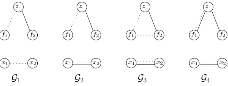
Definition 1[E-graphs].An E-graphGis a tripletG= V,E=,E=/, whereV is the set of vertices, and
E=(Equality edges) andE=/ (Disequality edges) are sets of unordered pairs of vertices.
From a given E-formulaϕEin Negation Normal Form (all negations are pushed to the atoms), we
construct theE-graphG(ϕE):G(ϕE)contains a vertex for each term-variable ofϕE, and an edge for
each equality or disequality ofϕE.
Given an E-graphG= V,E=,E=/, we denoteV(G)=V,E=/(G)=E=/ andE=(G)=E=. We use to denote the subgraph relation:HGif and only ifE=(H)⊆E=(G)andE=/(H)⊆E=/(G).
We say that an assignmentsatisfies an edgee=(a,b)(marked|=e) ife is an equality edge (e∈E=(G)) and(a)=(b), or ifeis a disequality edge (e∈E=/(G)) and(a) /=(b). We denote
|=Gifsatisfies all edges ofG.Gis said to be satisfiable if there exists somesuch that|=G. Example 1. The E-formula ϕE
1:(a=b)∧((c /=b)∨(a=c)) results in the E-graph depicted in
Fig. 1.
One may viewG(ϕE)as a conservative abstraction ofϕE, as it contains all the atomic equalities
appearingin ϕE and their polarities, yet has no representation for the Boolean relation between
them.
The property ofG(ϕE)that interests us the most is the fact that satisfaction ofϕE depends only
on the satisfaction of the sub-formulas represented by the edges ofG(ϕE). More formally,
Proposition 1. Given assignmentsandoverV(G(ϕE)),if for every edgeeofG(ϕE),|=e↔ |=e,
then|=ϕE↔|=ϕE.
This implies that if we want to check whetherϕEis satisfiable, it is sufficient to check one satisfying
assignment per satisfiable subgraph ofG(ϕE). More generally,
Definition 2[adequacy of assignment sets to E-graphs].Given an E-graphG, andR, a set of assign-ments toV(G), we say thatRis adequate forGif for every satisfiableHG, there is∈Rsuch that
|=H.
Example 2. The following set is adequate for the E-graph of Fig. 1:
R:= {(a←0,b←0,c←0),(a←0,b←0,c←1),(a←0,b←1,c←0)}.
In [18,15] we presented, together with Pnueli and Siegel, theRange-Allocationalgorithm that analyzes the E-graph in polynomial time and findsadequate domains, i.e., a set of values to each variable, from which it is possible to derive an adequate assignment set. Enumerating the possible assignments symbolically is left for the BDD package in the last stage. For example, adequate domains for Example 2 are
a→ {0},b→ {0, 1},c→ {0, 1}.
Note how the assignment sets of Example 2 can be derived from these domains. We will not re-peat the details of the Range-Allocation algorithm here. However, we should mention that the size of the allocated domains, which reflect the overall search-space in the last stage, grows mono-tonically with the E-graph that it reads as input. That is, given the E-graphsHand G such that HG, the Range-Allocation algorithm guarantees that the domain allocated for H is smaller or equal to the domain allocated for G. This clearly justifies the motivation behind the current work: we will build far smaller graphs that consequently result in drastically smaller search-spaces.
The property ofG(ϕE)stated in Proposition 1 is what makes this technique correct. However, we
can use a weaker property of E-graphs.
Definition 3[an E-graph satisfies an E-formula].For a satisfiable E-graphG, we say thatG|=ϕEifG
has the same edges (equality predicates) asϕE, and for every assignmentsuch that|=G,|=ϕE.
Less formally, this definition relates an Equality subgraph to the set of predicates that it represents: if the satisfaction of this set guarantees the satisfaction ofϕE, then we say that this subgraph satisfies ϕE.
Definition 4[adequacy of E-graphs to E-formulas].An E-graphG is adequate for E-formulaϕE, if
eitherϕEis not satisfiable, or there exists a satisfiableHGsuch thatH|=ϕE.
Clearly,G(ϕE)is adequate forϕE.
Example 3.If we remove the edge betweencandbin the E-graph of Fig. 1, the remaining E-graph is still adequate forϕE
1.
We claim:
Proposition 2.If E-graph G is adequate for ϕE,and assignment setR is adequate for G, then ϕE is
satisfiable iff there is∈Rsuch that|=ϕE.
Let us now rephrase the decision procedure for the satisfiability of an input EUF-formulasϕEUFas
(1) ReduceϕEUFto an E-formulaϕE such thatϕEis satisfiable if and only if there exists an
inter-pretation which satisfiesϕEUF.
(2) Construct the E-graphG(ϕE).
(3) Calculate an adequate domainRforG(ϕE).
(4) Check (symbolically) if any of the assignments inRsatisfyϕE.
Our suggested procedure replaces Steps 1 and 2 with a single step. The main idea is to exploit information which is only visible in the original formulaϕEUFbefore its reduction toϕE.
5. Reducing Uninterpreted Functions to Equality Logic
Given an EUF-formulaϕEUF, we wish to generate an E-formulaϕEsuch thatϕEUFis satisfiable iff ϕEis satisfiable.
We will use the followingEUF-formula throughout this section to illustrate the reduction:
ϕEUF
1 :=F(F(F(x1))) /=F(F(x1))∧ F(F(x1)) /=F(x2)∧ x2 =F(x1).
(4) For each function symbol (onlyF in this case) we number the function instances from the inside-out, and give equal indices to instances with syntactically equivalent arguments. Thus, the number-ingrespects the sub-term orderingofϕEUF. In other words, for every two function instancesF
i and
Fj, ifFiappears as a sub-term of the termFj(. . .)inϕEUF, then we must havei < j. This results in
ϕEUF
1 :=F4(F3(F1(x1))) /=F3(F1(x1))∧ F3(F1(x1)) /=F2(x2)∧
x2 =F1(x1).
(5) For function instance Fi ofϕEUF, define arg l(Fi)to be the term ofϕEUF correspondingto thel-th
argument ofFi.
Example 4.
arg1(F1)=x1 (6)
arg1(F4)=F3(F1(x1)). (7)
The followingtranslation is due to Bryant et al. [6,3]. We denote the resultingformula from this translation withT(ϕEUF).T(ϕEUF)is given by replacing the function instanceF
iinϕEUFwith the term
F夝 i for alli, F夝 i = f1 lT(argl(Fi))=T(argl(F1)), f2 lT(argl(Fi))=T(argl(F2)), ... ... fi−1 lT(argl(Fi))=T(argl(Fi−1)), fi true.
Note that since the numberingof the function instances respects the sub-term orderingofϕEUF, it
is guaranteed that no cyclic definition is possible. TheF夝symbols should be thought of as ‘place
holders’ only necessary for convenient notation. Practically only the expressions that they represent are present in the translated formula, in the form of ITE expressions as was shown before.
Example 5.GivenϕEUF
1 from Eq. 5,T(ϕEUF1 )is given by: T(ϕEUF 1 ):=(F4夝=/ F3夝)∧(F3夝=/ F2夝)∧(x2=F1夝), where F夝 1 :=f1; F2夝:= f1 x1=x2; f2 true; F3夝:= f1 F1夝=x1; f2 F1夝=x2; f3 true; F4夝:= f1 F3夝=x1; f2 F3夝=x2; f3 F3夝=F1夝; f4 true.
6. E-graph construction: an informal discussion
Given an EUF-formulaϕEUF, we wish to construct a minimal adequate E-graph forT(ϕEUF). In
this section we try to explain the intuition behind our suggested construction of E-graphs, which we termMinimal-E. In this section we will ignore ITE expressions, predicates, and Boolean variables
for simplicity. These will be handled in later sections.
For aϕEUF, a sub-formula or sub-term ofϕEUF, we definesimp(ϕEUF)to be the result of replacing
inϕEUFevery function instanceF
iby a new term-variablefi. For example:
Example 6.
simp(F4(F3(F1(y))))=f4, (8)
simp(arg1(F3))=f1, (9)
simp(ϕEUF
1 )=((f4=/ f3)∧(f3 =/ f2)∧(x=f1)). (10)
We will explain the intuition behind the construction with a series of attempts, each one improving upon the previous attempt. We begin with a naive approach in which we build a graph only according tosimp(ϕEUF). ConsiderϕEUF
5 : ϕEUF 5 :=F1(x1) /=F2(x2)∧((x1=x2)∨true) (11) for which simp(ϕEUF 5 ):=f1=/ f2∧((x1=x2)∨true) (12)
Fig. 2. An E-graph based onsimp(ϕEUF 5 ). and T(ϕEUF 5 ):=F1夝=/ F2夝∧((x1=x2)∨true) (13) together with: F1夝:=f1; F夝 2 := f1 x1=x2; f2 true.
Obviously any decent procedure will remove the right clause inT(ϕEUF
5 ), but thistruecan be hidden
as a more complex valid formula. Suppose that we build a graph only according to the top-level formula,simp(ϕEUF
5 ). The corresponding E-graph contains one disequality edge betweenf1andf2,
and one equality edge betweenx1andx2, as appears in Fig. 2.
A possible assignment set for this graph can contain the single assignment:
(x1,x2,f1,f2)←(0, 0, 2, 3) (14)
which does not satisfy T(ϕEUF
5 ). This is because the graph fails to represent the fact thatf1=/ f2
impliesx1=/ x2. Addinga disequality edge betweenx1andx2can solve this problem, since it forces
the allocated domain to include at least one assignment such as
(x1,x2,f1,f2)←(0, 1, 2, 3)
which satisfiesT(ϕEUF
5 )(an adequate domain can beR:x1→ {0},x2→ {0, 1},f1→ {2},f2→ {3}).
But how do we generalize this case? Suppose we say that we need to add a disequality edge between the argumentsxi,xj offi andfj if(fi,fj)∈E=/ and(xi,xj)∈E=. This indeed solves the
case ofϕEUF
5 , but consider nowϕEUF6 : ϕEUF
6 :=(F1(x1)=z)∧(F2(x2) /=z)∧((x1=x2)∨true), (15)
simp(ϕEUF
6 ):=f1=z∧(f2=/ z)∧((x1=x2)∨true). (16)
The E-graph forϕEUF
6 appears asG1in Fig. 3. As before dashed lines represent equality edges and
solid lines represent disequality edges. In the case ofϕEUF
Fig. 3. The iterative E-graph construction process.
we are left with the same problem, since a possible adequate domain for this E-graph can contain the single assignment:
(x1,x2,z,f1,f2)←(0, 0, 1, 1, 2)
which does not satisfyT(ϕEUF 6 ).
This is because there is no disequality edge betweenf1and f2, but nevertheless the disequality
between them isimpliedby the path throughz. So we need to generalize our rule in a way that it refers to disequalitypathsinstead of disequalityedges, and equalitypathsinstead of equalityedges. This will enable us to identifyimpliedequality and disequality requirements.
Definition 5[Equality Path].There is anEquality PathbetweenuandvinG, denotedu=∗
G v, if there
is a simple path inGbetweenuandvinE=.
Definition 6[Disequality Path].There is aDisequality PathbetweenuandvinG, denotedu /=∗ G v, if
there is a simple path inGbetweenuandvsuch that one edge in the path is fromE=/ and all other
edges are fromE=.
We can now define our first rule:
Rule 1.For fi and fj with arguments xi andxj, respectively, iffi =/∗Gfj andxi =∗Gxj, then add a
disequality edge betweenxi andxj.
Applyingthis rule toϕEUF
6 , we g etG2of Fig. 3, which solves this case. We proceed by considering a
similar EUF-formula,
ϕEUF
7 =(true∨(F1(x1)=z))∧(F2(x2) /=z)∧(x1=x2) (17)
G(simp(ϕEUF
7 ))is exactly the same as before (G1in Fig. 3, and Rule 1 adds the disequality edge(x1,x2)
to giveG2in Fig. 3. The problem here is that a satisfying assignmentmust satisfy(x1)=(x2), and
therefore(F夝
2 )=(F1夝). Since we also must have(F2夝) /=(z)to satisfy the formula, it implies (F夝
1 ) /=(z). This may not necessarily happen in any assignment in an adequate assignment set
for our E-graph. This is because in our E-graph there is no representation for the fact thatf1may
“override”f2, i.e., ifx1=x2 thenF2夝is evaluated tof1. If we add an equality edge betweenf1and f2it will solve the problem.G3of Fig. 3 is the result of adding this edge.
(Suggested) Rule 2.For fi and fj, withxi andxj their correspondingarguments, ifxi =∗G xj then
add the equality edge(fi,fj).
This indeed solves our problem, but is not the best that we can do. We added an equality edge between f1 and f2 in our example, but it is not really necessary. Instead, we can copy all edges
involvingf2 tof1. This is because there is no need forf1to be equal tof2 if their arguments are
equal to satisfyϕE, when usingBryant et al.’s reduction (because in this case bothF夝
1 andF2夝are
assigned the value off1). But ifF2夝 is assigned the value off1, then we need to make sure thatf1
can satisfy all the constraints overF夝
2 . Allowingf1to be equal tof2in the E-graph is only one way
to do this (the Range Allocation algorithm guarantees that every two variables with an Equality Path between them can satisfy the same constraints), but there is another way as well: simply copy all constraints overf2 tof1. Notice that this case is asymmetric: sincef1may overridef2, onlyf1
is required to respectf2’s requirements. The additional option can help us add less equality edges,
which in general impose larger allocated domains.
We therefore change the suggested rule above to the following rule:
Rule 2.Forfiandfj, wherei < j, withxi andxjtheir correspondingarguments, ifxi =∗G xjthen do
one of the following:
(1) add equality edge(fi,fj), or
(2) (a) for every equality edge(fj,w)add an equality edge(fi,w), and
(b) for every disequality edge(fj,w)add a disequality edge(fi,w).
And so, in our example, instead of addingan equality edge(f1,f2), we can add a disequality edge (f1,z), which results inG4of Fig. 3. The formalization of applying Rule 2 requires a special graph
calledassignment graphthat we will show in the next section.
Note that the asymmetry betweenf1andf2suggests that there is another optimization problem
here: the function elimination order (the indices that we give to function instances) is not unique, as there are many orders that respect the sub-term orderingbetween function applications. We can do better than just selectingbetween them arbitrarily if we select an order that minimizes the resultingallocated domain (minimizingthe number of added dashed edges by Rule 2 is a good strategy to achieve this goal). This type of optimal ordering is the main idea behind the Robust Positive Equality method of [13], although there the goal was somewhat different. We adopt their strategy forMinimal-Enevertheless to generalize their result. More details about this optimization
problem appear in Appendix C. Finally, consider the simple formula:
ϕEUF
8 =F1(x1) /=F2(x2). (18)
The E-graph now only containsx1,x2,f1, andf2as variables and only one disequality edge between f1andf2. Rule 1 does not apply here because there is no equality path betweenx1andx2. We need
to check whether an adequate range for this graph satisfiesT(ϕEUF 8 ): T(ϕEUF
and
F1夝:=f1 F2夝:=
f1 x1=x2; f2 true.
A possible adequate domain for the corresponding graph contains just one assignment, for example:
(x1,x2,f1,f2)←(0, 0, 0, 1). (20)
This assignment does not satisfy T(ϕEUF
8 ), and so our attempt fails. What we need to do is to
ensure that the allocated domain guarantees a certain diversity property, i.e., that unless the graph requires otherwise, it gives different values to different variables. The good news about this requirement is that it does not increase the size of the necessary domain. Let us denote this rule as Rule 3:
Rule 3.Ifu=∗Gvdoes not hold then add a disequality edge betweenuandv. This rule should be applied last, after we know all the requirements over the edges.
Now, applyingRule 3 results in an E-graph which is a solid clique between the nodes{x1,x2,f1,f2}.
A possible adequate assignment set for this E-graph contains one assignment,
(x1,x2,f1,f2)←(1, 2, 3, 4)
which satisfiesT(ϕEUF 8 ).
Summary.Minimal-Econstructs an E-graph from an EUF-formulaϕEUFas appears in Algorithm 1.
Notice that this construction somewhat reminds acone-of-influencereduction, since insimp(ϕEUF)
the arguments of Uninterpreted Functions disappear, and then only edges emanating from edges already in the E-graph are added.
Algorithm 1TheMinimal-Ealgorithm for an EUF-formulaϕEUFwithout ITE expressions,
predi-cates, and Boolean variables. (1) ConstructG(simp(ϕEUF)).
(2) Apply Rules 1 and 2 until no new edges are added. (3) Apply Rule 3.
The construction so far did not consider the case in which we haveITEexpressions in theoriginal
formula(not those that result from the reduction of Uninterpreted Functions), which complicates
things. We delay the treatment of these expressions to Section 8. In that section we will also give the full construction and proof, which involves new kind of graphs calledAssignment Graphs. This is the topic of the next section.
7. Assignment Graphs
We now return to work our way towards our main result, a graph construction for general EUF-formulas that will generalize the results of [3]. We will also need a new kind of graph, called an Assignment Graph, or A-graph for short.
Definition 7 [A-graph]. An A-graph is a quadruple G↑ = V,E=,E=/,E↑, where V is the set of
vertices,E= andE=/ are sets of unordered pairs of vertices andE↑(Assignment edges) is a set of
ordered pairs of vertices.
Given an A-graphG↑ = V,E=,E=/,E↑, we denoteV(G↑)=V,E=/(G↑)=E=/,E=(G↑)=E=
andE↑(G↑)=E↑. We denotea→聻
G↑b, if there is a directed path (possibly of length 0) of assignment
edges fromatobinG↑.
Assignment edges (edges inE↑) serve as a weak form of equality. Intuitively, the meaningof an assignment edge fromatobis that the value ofbis ‘overridden’ bya’s value, i.e., all edges adjacent tobare checked againsta’s value in addition to beingchecked againstb’s value. The relevance of this term to Rule 2 is clear.
Formally, for an assignmentand an A-graphG↑, we denote|=G↑if for everya→聻
G↑band c→聻
G↑d:
(1) If(b,d)∈E=(G↑),(a)=(c).
(2) If(b,d)∈E=/(G↑),(a) /=(c).
Note that|=G↑implies thatsatisfies all equality and disequality edges ofG↑(by settingthe paths to be of length 0). For A-graphG↑denoted byflatEq (G↑) the E-graph was obtained by replacing all assignment edges ofG↑by equality edges. We say that an A-graphG↑is satisfiable
if flatEq (G↑) is satisfiable. This is not the most natural definition, but we will need it for our
translation from A-graphs to E-graphs (Section 9). Note that if |=flatEq (G↑) then |=G↑. However, the fact that|=G↑does not necessarily imply that|=flatEq (G↑). For example, the assignment (x,y,z)←(1, 2, 3) satisfies the A-graph G↑that has one disequality edge between y
and z and one assignment edge fromx toy. On the other hand, this assignment does not satisfy
flatEq (G↑).
For an E-formulaϕEand a satisfiable A-graphG↑, we denoteG↑ |=ϕEif for every assignment
such that|=G↑we have|=ϕE. The followingdefinitions are the exact analogof the definitions
associated with E-graphs:
Definition 8[adequacy of A-graphs to E-formulas].An A-graphG↑is adequate for E-formulaϕE, if
eitherϕEis not satisfiable, or there exists a satisfiableH↑G↑such thatH↑ |=ϕE.
Definition 9[adequacy of assignment sets to A-graphs].Given an A-graphG↑, andR, a set of assign-ments toV(G↑), we say thatRis adequate forG↑if for every satisfiableH↑G↑there is∈R
such that|=H↑.
The analogous proposition follows:
Proposition 3.If A-graphG↑is adequate forϕE,and assignment setRis adequate forG↑,thenϕEis
In the followingsection, given an EUF-formulaϕEUF, we will construct an A-graphG↑such that
G↑is adequate forT(ϕEUF). In Section 9 we will show how to create an E-graphGfromG↑, such that
ifRis adequate forGit is also adequate forG↑. These two procedures combined with a procedure for finding an adequate assignment set for an E-graph give us a more efficient decision procedure for the satisfiability of EUF-formulas.
8. The minimal A-graph construction
In this section, we describe and prove the A-graph construction for general EUF-formulas (in-cludingITE expressions). Note that we still do not handle predicates and Boolean variables. They will be discussed in Section 11.
Example 7.In the followingexample we writeFi(·)wheneverFi’s arguments were already specified
for better readability:
ϕEUF
9 :=F2(ITE(F1(b)=u, a, b))=u∧
F3(F2(·)) /=F4(ITE(a=b, u, a)). (21)
The resultingE-formula is:
T(ϕEUF 9 ):=(F2夝=u)∧(F3夝=/ F4夝) (22) A1 :=b F1夝:=f1; A2:=ITE(F夝1 (b)=u, a, b) F2夝:= f1 A2 =A1; f2 true; A3:=F2夝 F3夝:= f 1 A3 =A1; f2 A3 =A2; f3 true; A4:=ITE(a=b, u, a) F4夝:= f1 A4 =A1; f2 A4 =A2; f3 A4 =A3; f4 true;
whereAi is the term correspondingtoARG1(Fi)in the translated formula.
In the followingdiscussion the distinction betweenFi,fi, andFi夝is crucial.Fi is theith function
instance of an EUF-formulaϕEUF (accordingto our predetermined numberingof the function
in-stances ofϕEUF).f
i is the term-variable ofT(ϕEUF)that was introduced by the reduction, andFi夝is
the term ofT(ϕEUF)which replacesF
i inϕEUF.
8.1. Definitions
We start with some notations for an EUF-formulaϕEUF, assignmentto the variables ofT(ϕEUF),
and an A-graphG↑. For this purpose, we will use the followingexample assignment toT(ϕEUF 9 )’s
variables:
(a)=0, (b)=0, (u)=1,
(1) For a termtofT(ϕEUF), define(t)to be the evaluation oftunder. Example 8.InϕEUF 9 , (A1) = (b) =0, (A2)= (a) =0, (A3)= (F2夝)=1, (A4)= (u) =1, (F夝 1 )= (f1) =1, (F2夝)= (f1) =1, (F夝 3 )= (f3)=3, (F4夝)= (f3)=3.
(2) For a term-variablevofT(ϕEUF), definesource
(v):
•Ifvis an original term-variable ofϕEUFthensource
(v)=v.
•Ifv≡fj, then take the minimalisuch that for alll,(T(argl(Fi)))=(T(argl(Fj))), and set
source(v)=fi.
Example 9.InϕEUF 9 :
source (a)=a source (b)=b source (u)=u
source (f1)=f1source (f2)=f1source (f3)=f3source (f4)=f3
(3) Define the assignmentˆ to be:
•Forv, a term-variable ofϕEUF, set(v)ˆ =(v).
•Forv≡fi,(fˆ i)=(Fi夝).
Notice that (v)ˆ =(source(v)). ˆ can be seen as the real assignment induced by , and
forϕEUFa sub-term or sub-formula ofϕEUFwe have(T(ϕEUF))= ˆ(simp(ϕEUF)). In particular |=T(ϕEUF)iffˆ |=simp(ϕEUF).
Example 10.
ˆ
(a)=0, (b)ˆ =0, (u)ˆ =1,
ˆ
(f1)=1, (fˆ 2)=1, (fˆ 3)=3, (fˆ 4)=3.
(4) For a termtofϕEUF, definevals(t)to be:
•Iftis a term-variable thenvals(t)= {t}.
•Ift=Fi(. . .)thenvals(t)= {fi}.
•Ift=ITE(cond, t1, t2)thenvals(t)=vals(t1)∪vals(t2).
Notice that(T(t))= ˆ(v)for somev∈vals(t), dependingon the evaluation of the Boolean conditions in the relevant ITE terms.
Example 11.In our exampleϕEUF 9 :
•vals(F3 (. . .))= {f3}
•vals(ITE(a=b, u, a))= {u,a} •vals(arg1 (F2 ))= {a,b}.
(5) Foru,v∈V(G↑), we marku=∗G↑viffu=∗flatEq (G↑)v, andu /=∗G↑viffu /=∗flatEq (G↑)v. Recall that for an A-graphG↑,flatEq (G↑) isG↑where all assignment edges are replaced by equality edges.
We extend this definition to sets of verticesU1andU2, and markU1=∗G↑U2if there exists some u1∈U1andu2∈U2such thatu1=∗G↑u2.
8.2. A-graph construction
Given an EUF-formulaϕEUFwe construct an A-graphG↑as described by Algorithm 2.
Algorithm 2The A-graph construction algorithm, which is the first stage ofMinimal-E.
(1) Let the vertices be the set of term-variables ofT(ϕEUF).
(2) Add as minimum all edges ofG(simp(ϕEUF))toG↑2.
(3) For everyFiandFjsuch thati < j, if for alllvals(argl(Fi))=∗G↑vals(argl(Fj)), then add the
followingedges:
•Add(fi,fj)toE↑(G↑).
•Iffi =/∗G↑fjthen for alll, for allvi ∈vals(argl(Fi))andvj ∈vals(argl(Fj))add edge(vi,vj)
toE=/(G↑). Also markFi andFjascritical.
(4) For every critical Fi, if for somelthe termt=ITE(cond, t1, t2)appears in simp(arg l(Fi)),
then add all edges ofG(cond)andG(¬cond)toG↑. Also addcondto setC (which is initially empty).
(5) Repeat Steps 3 and 4 until convergence. (6) For everyu,v, such that¬(u=∗
G↑v), add edge(u,v)toE=/(G↑). Denote all these edgesfree(in
Section 10 we prove that they do not increase the state-space).
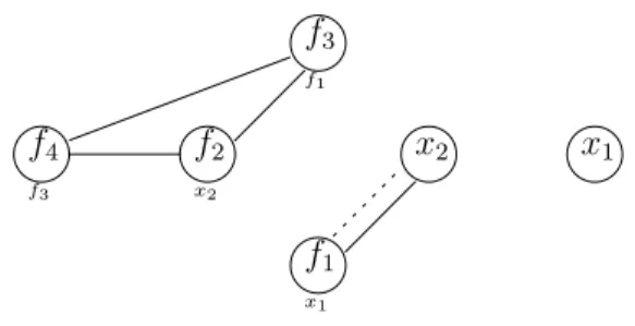
Example 12.For ϕEUF
9 , the edges are added as follows:
(1) In Step 2, we add(f3,f4)toE=/(G↑)and(u,f2) toE=(G↑). The state ofG↑at this point is
described in Fig. 4A. In this figure, under a vertex corresponding to function variablefi, we
have added the list of vertices invals(arg1(Fi)). (2) In Step 3, we add the followingedges:
•(f1,f2)toE↑(G↑)sinceb∈vals(arg1(f1))andb∈vals(arg1(f2)).
•(f2,f4)toE↑(G↑)sincea∈vals(arg1(f2))anda∈vals(arg1(f4)).
•(f3,f4)is added toE↑(G↑)sincef2 =G∗↑u. Also, sincef3 =/∗G↑f4,F3andF4are marked as
critical, and(f2,u)and(f2,a)are added toE=/(G↑)
(3) SinceF4was marked as critical,(a=b)∈C. Therefore, in Step 4, we add(a,b)to bothE=(G↑)
andE=/(G↑).
(4) Now (this was not the case before), sincea=∗G↑b, we add(f1,f4)toE↑(G↑). See part B of
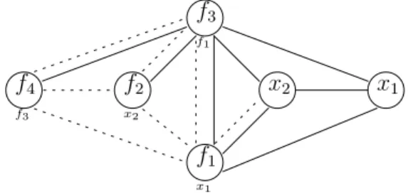
Fig. 4.
(5) We now add all Free-Edges. For every x∈ {a,b} and y ∈ {f1,f2,f3,f4,u} we add (x,y) to E=/(G↑).
Fig. 4. (A)ϕEUF
9 ’s A-graph after Step 2. (B)ϕEUF9 ’s A-graph after convergence (before Free-Edges are added).
Notice that throughout the construction we did not examine the condition of the ITE term appearing in the argument ofF2, sinceF2was not marked as critical. This is an example of the “cone of influence”
effect we were aimingfor.
Soundness: The followingtheorem states that the construction is sound.
Theorem 1. The A-graphG↑constructed for the EUF-formulaϕEUF is adequate forT(ϕEUF).
The proof of this theorem appears in Appendix D. 9. Transforming A-graphs to E-graphs
In the previous section we showed how to construct an adequate A-graphG↑forT(ϕEUF). Next,
we would like to generate an adequate set of assignments forG↑. Since the methods proposed in [15,19] calculate an adequate set of assignments only for an E-graph, we proceed in the following manner: given an A-graphG↑, we construct an E-graphGsuch that if assignment setRis adequate forGit will also be adequate forG↑. In principle, we could have usedflatEq (G↑)as the E-graph correspondingto the A-graphG↑. However, we can do somewhat better.
For two verticesuandv, we denotev⊆Gu, if
•for every(v,w)∈E=(G),(u,w)∈E=(G),
•for every(v,w)∈E=/(G),(u,w)∈E=/(G).
That is,uinherits any (E=∪E=/)-edge that departs fromv. Algorithm 3 transforms A-graphs to
E-graphs.
Algorithm 3Transforming A-graphs to E-graphs (1) Initially,G= V(G↑),E=(G↑),E=/(G↑).
(2) While there are verticesu,v, such that(u,v)∈E↑(G↑)and neither(u,v)∈E=(G)norv⊆Gu,
choose one of the followingoptions: (a) add edge(u,v)toE=(G),
(b)•for every(v,w)∈E=(G)add(u,w)toE=(G),
Theorem 2.IfRis adequate forGthen it is also adequate forG↑.
Proof.Take some satisfiableH↑G↑. We construct a satisfiableHGsuch that if|=Hthen
|=H↑.
SinceH↑is satisfiable, there is somethat satisfiesH↑where all ofH↑’s assignment edges are replaced by equality edges (recall the definition of the satisfiability of an A-graph). We construct a subgraphHGand show that|=H.
Start with E=(H)=E=(H↑), and E=/(H)=E=/(H↑). Clearly, at this stage |=H. For every
edge(u,v)∈E↑(H↑)(notice that(u)=(v)):
•If(u,v)∈E=(G)add(u,v)toE=(H). Obviously|=Hafter this addition.
•Otherwise, we have thatv⊆Gu. Add the followingedges toH:
(1) for every(v,w)∈E=(H)add(u,w)toE=(H),
(2) for every(v,w)∈E=/(H)add(u,w)toE=/(H).
Since |=H before this step, and (v)=(u), it is easy to see that also after this step
|=H.
We now prove that if |=Hthen|=H↑. Take somea→聻
H↑bandc→聻H↑d. We need to prove
that:
•If(b,d)∈E=(H↑)then(a)=(c).
•If(b,d)∈E=/(H↑)then(a) /=(c).
To simplify the proof we weaken the definition of =∗ and =/∗, so that the paths need not be
simple. Notice that under this definition we still have:
•Ifx=∗
Hythen(x)=(y).
•Ifx /=∗Hythen(x) /=(y).
We will therefore prove:
•If(b,d)∈E=(H↑)thena=∗Hc.
•If(b,d)∈E=/(H↑)thena /=∗Hc.
We will prove this by induction on the sum of the lengths of the assignment edge paths froma
toband fromc tod. If this sum is 0, thena=b andc=d, and since we copied all equality and disequality edges ofH↑toH, the claim follows.
If this sum is greater than 0, then one of these paths is of length greater than 0. Without loss of generality, assume this is the path betweenaandb. Mark byathe next vertex afterain the path to
b(this may bebitself). Accordingto our induction hypothesis:
•If(b,d)∈E=(H↑)thena=∗Hc.
Fig. 5. The A-graph ofϕEUF 1 .
Since(a,a)∈E↑(H↑), we have one of the two cases:
(1) (a,a)∈E=(H). But then clearly a satisfies the two claims, since we simply prolong
the patha =∗
H c(in the first case) ora=/H∗ c(in the second) by the equality edge(a,a).
(2) Otherwise, we know thata ⊆
Ha. This time instead of prolonging these paths, we replace their
first edge. For example, if(b,d)∈E=/(H), thena =/∗Hc. This means there is a path froma to
cinHconsisting of equality edges except one edge which is a disequality edge. Take the first edge in this path(a,x)and replace it by the same type (equality or disequality) of edge(a,x).
We know this edge is inH, sincea⊆Ha.
We showed a general method for translating A-graphs to E-graphs. When using this method one has to choose between the two options for every assignment edge: either replace it by an equality edge, or copy all edges of the end vertex to the start vertex.
Note that if the original EUF-formulaϕEUFis in Positive Equality then the A-graph constructed
in Section 8.2 contains no equality edges, and therefore we can translate it to an E-graph with no equality edges. An adequate set of assignments for such an E-graph contains just one assignment in which every variable is assigned a distinct constant. This is exactly the result of [3].
In our implementation, we use a greedy approach for choosing between the options, where we try to minimize the number of equality edges of the resulting E-graph. In the case of Positive Equality formulas, we therefore get the optimal result of [3].
Example 13. We demonstrate the transformation with the help ofϕEUF
1 , the EUF-formula that was
first presented in Section 5. The resultingA-graph ofϕEUF
1 from the construction appears in Fig. 5,
and the result of transforming it to an E-graph (using the greedy approach) is presented in Fig. 6. This graph has an adequate set of assignments that consists of two assignments.
10. Free-Edges do not increase the state-space
Recall the last step of our graph construction: If ¬(u=∗G↑v) then the disequality edge(u,v)is added toG↑. We call these edges free because they do not impose any increase in the size of the assignment setRthat is adequate forG↑.
Given an E-graphG(we will handle A-graphs later) and a setRthat is adequate forG, we construct an assignment setRthat is adequate forG, whereGis equal toGplus all Free-Edges. We will show
Fig. 6. An E-graph obtained from the A-graph ofϕEUF 1 .
DefineC(G)= {C1,C2,. . .} to be the set of connected components of the graphV(G),E=(G).
Notice thatu=∗
G viff there is someisuch thatu,v∈Ci. Take some numberN such that for every ∈Rand everyv∈V(G),N >2·(v). For∈Rwe defineto be the assignment that satisfies:
∀i∀v∈Ci, (v)=(v)+i·N.
DefineR = {|∈R}.
Claim 1.Ris adequate forG.
Proof.TakeH G.His composed of anHGplus some Free-Edges ofG. SinceRis adequate for
H, there exists∈Rsuch that|=H. We claim that|=H. Take some edge(u,v)ofH. There are Ci,Cj ∈C(G)such thatu∈Ciandv∈Cj. We have that(u)=i·N +(u)and(v)=j·N +(v).
Subtractingone from another we get:
(v)−(u)=(i−j)·N +(v)−(u).
•Ifi /=j then(u,v)must be a disequality edge (either free or originally inG). SinceN >|(u)−
(v)|we get that|(u)−(v)|>|(i−j)| ·N −N. Sincei /=jwe have that|(u)−(v)|>0,
implying(u) /=(v).
•Ifi=j, thensatisfies edge(u,v)(equality or disequality). Also(u)−(v)=(u)−(v), and
therefore also satisfies this edge.
Thus, adding Free-Edges to E-graphs does not increase the size of the assignment set. In the case of A-graphs, if we examine the transformation to E-graphs that we presented in Section 9, we see that if¬(u=∗G↑v)in the original A-graph, then also¬(u=∗G v)in the resultingE-graph. Therefore, the Free-Edges that we add to the original A-graph appear as Free-Edges in the resulting E-graph, and as we have just shown, it will not increase the size of the resultingassignment set.
11. Uninterpreted Predicates
Up to now we assumed that there are no predicate symbols or Boolean variables in the formula. We will justify this by showinghow we simulate predicates usingUninterpreted Functions (Boolean
Table 1
New vs. old E-graph construction
Example ME-finished [15]-finished ME-space [15]-space Num. vars
15 121 121 13 22 × 2 9.8×1046 114 25 × 1 5.9×1047 114 27 2 11,520 26 43 × 4 3.4×10108 160 44 4 2.5×10¹¹ 46 46 2 1.6×10²² 67 47 1 4.9×10⁹ 52
variables are merely predicates with 0 arguments). GivenϕEUF, an EUF-formula with uninterpreted
predicates, we transformϕEUFtoϕEUFwithout uninterpreted predicates.
For every predicate symbolP inϕEUF, take a new function symbolFP and a new term-variable trueP. Now replace inϕEUFevery occurrence ofP(. . .), by(FP(. . .)=trueP)to getϕEUF. It is not hard
to see thatϕEUF is satisfiable if and only ifϕEUFis.
The problem we are facingis that instead of addinga Boolean variable for each predicate instance (as suggested in [3]), we added a term-variable and possibly increased the state-space for checking
ϕEUF. But a more careful examination proves that this is not the case.
Note that in the A-graph ofϕEUF, all the new variables introduced for predicate P are isolated
(there are no edges between them and any of the other variables). Therefore we can find an adequate assignment set for each such predicate separately from each other and from the assignment set for the original graph (which is unaffected by this addition). We first transform the component’s A-graph to an E-graph by replacing all assignment edges by equality edges (this is a valid transformation accordingto Section 9). In our case the graph of the component of some predicateP cannot contain disequality edges other than(fP
i ,trueP). An adequate set of assignments for this kind of E-graph is
given by letting each variable range over{0, 1}, and settingtrueP to be the constant 1.
The state-space is therefore not increased. In fact this method gives us the ability to treat predicates with the new method we used for functions, achievinga similar cone-of-influence effect.
12. Experimental results and conclusions
As was mentioned earlier, the graphs that are generated byMinimal-Eare always contained or
equal to the graphs that were generated in [15], and therefore result in a smaller state-space. Since both algorithms are polynomial, we can considerMinimal-Eas dominant over [15].
Minimal-Eis also dominant over Positive Equality and Robust Positive Equality [3,13], since
it always assigns a single constant to the same terms that are assigned single constant by their analysis, but much smaller ranges to other terms. Given the variables{v0,. . .,vn}belonging to the
non-positive part, the Positive-Equality algorithm in [3,13] assign variable vi the range {1,. . .,i},
resultingin a state-space ofn!, while we use the Range-Allocation algorithm, which searches this state-space only in the worst case.
Table 2
Results with six competingdecision procedures
Example ICS UCLID CVC CVC-Lite SVC SIMPLIFY
15 1.1 1.8 1.0 4.1 1.9 112.1 22 1.74 33.92 3 549.15 16.25 × 25 1.04 10.54 1.4 × 23.53 × 27 0.22 1.11 0.61 0.1 0.05 6.52 43 128.79 90.87 437.13 × 56.83 × 44 0.33 2.64 0.85 0.21 0.09 5.99 46 0.41 4.02 0.7 0.18 0.2 10.61 47 0.18 8.14 2.16 0.20 1.91 2.03
×indicates run time of over an hour.
We implementedMinimal-Eand combined it with the Range-Allocation algorithm of [15] to
con-struct a new procedure for checkingsatisfiability of EUF-formulas in thecvttool, which performs
Translation Validation of both DC+ to C and Sildex to C optimizingcompilers.3 We compared our decision procedure with that of [15] on dozens of industrial examples generated as part of the Euro-pean SACRES and SafeAir projects (cvtis part of the tool-set that was developed in these projects).
The results appear in Table 1, where the prefix ME denotes the results obtained byMinimal-E, and
[15] the results of Range-Allocation as in [15]. Space denotes the resulting assignment set size. Since in all cases the verification procedure either proves that the formula is valid in less than 1 s, or runs out of memory, we do not write the exact runningtime. Instead we writeif the run completed, and×if it did not. Num. vars denotes the number of variables in the example. There are also many examples for which both methods generate very small domains that take almost no time to explore, which we omit from the table. As can be seen from the table,Minimal-Ehas a significant effect on
the state-space size. Indeed, by usingthis method we were able to verify formulas which we could not with the previous method. In fact, these examples were generated by decomposing large Trans-lation Validation verification tasks. NowMinimal-Everifies these tasks without decomposition at
all in a few seconds.
We also ran these benchmarks with six of the leadingdecision procedures to date: ICS [11], Uclid[7,14],CVC[21], andSIMP.4 None of these tools performed as well asMinimal-Eon these
benchmarks (Table 2).
All of these tools solve richer logics than just Equality Logic, and therefore the comparison cannot be considered as entirely fair: combiningtheories imposes an overhead which our tool does not have. Another difference is that our tool is the only one from this set, as far as know, that is based on (multi-typed) BDDs rather than on SAT.
12.1. Conclusions
We presentedMinimal-E, an algorithm for deciding EUF formulas, which generalizes and
im-proves the Positive Equality method of Bryant et al. [3] and the Range Allocation method of Pnueli
3DC+ and Sildex are popular synchronous languages in the European avionics industry.