University of Richmond University of Richmond
UR Scholarship Repository
UR Scholarship Repository
Honors Theses Student Research
2020
Computer-Assisted Coloring-Graph Generation and Structural
Computer-Assisted Coloring-Graph Generation and Structural
Analysis
Analysis
Wesley SuFollow this and additional works at: https://scholarship.richmond.edu/honors-theses
Part of the Computer Sciences Commons, and the Mathematics Commons
Recommended Citation Recommended Citation
Su, Wesley, "Computer-Assisted Coloring-Graph Generation and Structural Analysis" (2020). Honors Theses. 1510.
https://scholarship.richmond.edu/honors-theses/1510
This Thesis is brought to you for free and open access by the Student Research at UR Scholarship Repository. It has been accepted for inclusion in Honors Theses by an authorized administrator of UR Scholarship Repository. For more information, please contact [email protected].
Computer-Assisted Coloring-Graph
Generation and Structural Analysis
Wesley Su
Computer Science Honors Paper1
Department of Mathematics and Computer Science Universty of Richmond
May 2020
This paper is part of the requirements for the honors program in computer science. The signatures below, by the advisor, a departmental reader, and the departmental honors representative, demonstrate that Wesley Su has met all the requirements needed to receive honors in computer science.
Advisor – Prateek Bhakta
Reader – Jory Denny
ABSTRACT
Graphs are a well studied construction in discrete math, with one of the most common areas of study being graph coloring. The graph coloring problem asks for a color to be assigned to each vertex in a graph such that no two adjacent vertices share a color. An assignment of k colors that meets these criteria is called a k-coloring. The coloring graph Ck(G) is defined as the graph where every vertex represents a
valid k-coloring of graph G and edges exist between colorings that di↵er by one vertex. We call graph G the base graph of the k-coloring graph Ck(G). A primary
point of interest in coloring graph research is that of connectivity, and specifically, biconnectivity. To assist this research, we wrote software to compute and display coloring graphs. The software package allows the user to construct base graphs in a GUI. After construction, a fast backtracking algorithm with bit-arithmetic is used to compute all possible colorings of the base graph. To aid understanding of biconnectivity, we use an enhanced version of Robert Tarjan’s cut-vertex algorithm to identify biconnected components in the coloring graph and build a block-cut tree, or metagraph. The software has been useful in coloring graph research, especially for finding counter examples to hypotheses since base graphs can be randomly generated in mass numbers.
DEDICATION
This thesis is dedicated to my grandfather Aaron Su, who has inspired me like no one else to be the best possible version of myself.
ACKNOWLEDGEMENTS
I would never have even started writing this thesis without the encouragement of my advisor Prateek Bhakta, who originally encouraged me to join the honors program at UR and assist with this project. He has aided me in numerous ways, including teaching me how to program as a freshman, teaching me algorithms as a junior, and helping me design and implement this software last summer.
I would also like to thank my classmates Maxine Xin and Aalok Sathe. Maxine wrote an alpha version of this software two summers ago from which I learned many key concepts. She has also been active in formally documenting structural research of coloring graphs, making me feel less guilty about only caring about the CS. Aalok took on all the tedious programming that I didn’t want to do. He wrapped the C++ code in SWIG so that the program could be run in Python and easily distributed. He also learned the Javascript necessary for the program to run in a web browser with a real UI.
Professors Heather Russell and Sara Krehbiel have both helped organize team meetings and given me tasks to keep me focused, especially this past semester when Dr. Bhakta was on sabbatical. Jory Denny advised Aalok and me on how to structure our C++ code, and without his advice, we may never have gotten it working.
TABLE OF CONTENTS Page ABSTRACT TITLE . . . ii DEDICATION . . . iii ACKNOWLEDGEMENTS . . . iv TABLE OF CONTENTS . . . v LIST OF FIGURES . . . vi 1. INTRODUCTION . . . 1 1.1 Research Contribution . . . 3 1.2 Outline . . . 3
2. PRELIMINARIES AND RELATED WORK . . . 4
2.1 Preliminaries . . . 4
2.2 Related Work . . . 8
2.2.1 Dancing Links . . . 9
2.2.2 Tarjan’s Algorithm for Finding Articulation Points . . . 10
3. COLORING GRAPH GENERATION . . . 15
3.1 Computing Coloring Graph Vertices . . . 15
3.2 Computing Coloring Graph Edges . . . 21
4. METAGRAPH GENERATION . . . 25
4.1 Modifying Tarjan’s Algorithm . . . 25
4.2 The UI . . . 26
5. FUTURE DIRECTION . . . 29
5.1 Design Improvements . . . 29
5.2 Implementation Improvements . . . 30
LIST OF FIGURES
FIGURE Page
1.1 On top, a graph G, on the left, aninvalid 2-coloring ofG, and on the right, a valid 2-coloring of G. . . 2 1.2 A coloring graph with k = 3 . . . 2 2.1 A graph with 6 vertices and 9 edges. . . 4 2.2 A graph divided into two biconnected components by a central cut
vertex. Removing the cut vertex would disconnect the graph. . . 6 2.3 The metagraph of the graph in Figure 2.2. Note thatCUThas its own
vertex but is also included in both biconnected components, as cut vertices are part of both biconnected components that they divide. . . 6 2.4 An isomorphism between two graphs, where f(A) = 1, f(B) = 2, etc. 8 2.5 Tarjan’s algorithm partway through execution. The DFS traverses in
alphabetical order. Edges already traversed are marked in red. Known cut vertices are marked in green. Ordered pairs show (depth, lowpoint). 11 2.6 Tarjan’s algorithm partway through execution. At the current point in
time, the algorithm is returning from a child toNow, with the lowpoint of the child being greater than or equal to the depth of Now. Therefore
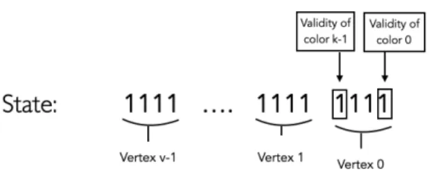
Nowwill be marked as a cut vertex. By the rules of DFS, the red edges are all impossible. . . 13 3.1 A visual representation of how the state bitstring is indexed for a
graph with size V and k = 4. This same indexing is used for the
assignment bitstring. . . 16 4.1 An example of coloring graph generation and analysis in the software.
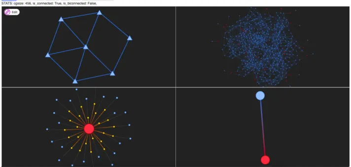
In the top-left, the user may construct a base graph. The top-right shows the coloring-graph. The bottom-left shows the metagraph. The bottom-right shows isomorphism classes of o↵shoots from the central component. . . 28
1. INTRODUCTION
Graph coloring is a well studied problem with applications in scheduling , elec-trical engineering, compiler optimization, and many other areas [14, 7]. The graph coloring problem asks, ”Given a graphGand a number of colorsk, how can we assign a color to each vertex such that no adjacent vertices share a color?” Any assignment of k colors that meets these criteria is called a valid k-coloring. Figure 1.1 shows both an invalid and valid k-coloring of a small graph with k = 2.
We are interested in a graph-coloring reconfiguration problem. Reconfiguration problems seek to switch between two allowable solutions to a problem in a series of steps, where each intermediate configuration is also a valid solution to the problem. Many examples of reconfiguration problems can be found in [11]. In the context of graph coloring, we try to reconfigure one valid coloring into another. Each step in the reconfiguration process changes the color of one vertex. The reconfigurations of graph-coloring can be represented using a a structure called a coloring graph. The k-coloring graph Ck(G) is the graph where each vertex in Ck(G) represents a valid
coloring of G. Edges exist between vertices in Ck(G) if the colorings represented by
those vertices di↵er by the color of exactly one vertex of G. We call graph G the
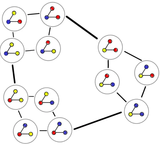
base graph of the k-coloring graph Ck(G). Figure 1.2 shows the 3-coloring graph of
the graph in Figure 1.1.
We want to know how easily any solution to the graph coloring problem can be reconfigured into any other solution. In other words, we want to know about the connectivity of coloring graphs. It is helpful to visualize graphs in order to understand their high level connectivity. In the context of coloring graphs, the desire for visualization presents a problem. Most of the interesting concepts in coloring
Figure 1.1: On top, a graph G, on the left, an invalid 2-coloring of G, and on the right, a valid 2-coloring of G.
graph connectivity only arise when the coloring graphs are too big to compute by hand. Finding even one valid coloring of a graph is an NP-hard problem [12], and the number of valid colorings can grow exponentially with the size of the graph and the number of colors. Therefore, understanding the structure of coloring graphs is a computationally intensive process.
1.1 Research Contribution
To aid the study of coloring graphs, we wrote a software package to compute, visualize, and analyze the structure of coloring graphs. The software package allows the user to construct base graphs in a GUI. After construction, a fast backtracking algorithm with bit-arithmetic is used to compute all possible colorings of the base graph. To aid with connectivity visualization, we use an enhanced version of Robert Tarjan’s cut vertex algorithm to construct a block-cut tree, or metagraph, of the coloring graph [10].
1.2 Outline
Chapter 2 of this thesis explains the necessary definitions and properties of col-oring graphs to understand the goals of our software. It also explains previous algorithms used in connectivity and coloring research. Chapter 3 explains how we construct coloring graphs quickly and store them using minimal space. Chapter 4 shows how we modify Tarjan’s cut vertex algorithm to compute a metagraph. Chap-ter 5 explains how the software may continue to be improved in the future.
2. PRELIMINARIES AND RELATED WORK
Some knowledge of graph theory is necessary to understand this paper. Here we formally introduce some concepts in graph connectivity and graph coloring. We also discuss some previous work related to graph coloring as context for our software.
2.1 Preliminaries
We begin by formally defining a graph.
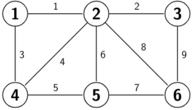
Definition 2.1.1. AgraphG= (V, E), whereV andE are sets. The setV contains elements called vertices. The elements in set E are pairings of two vertices in V. The elements in E are called edges (See Figure 2.1).
A useful definition before defining connected and biconnected graphs is the defi-nition of a path in a graph.
Definition 2.1.2. Given a graph G = (V, E), a path is a sequence of distinct vertices (v1, v2...vn) and a sequence of distinct edges (e1, e2...en 1) such that each
edge ei ={vi, vi+1}, and ei 2E.
Connected and biconnected graphs can now be defined in terms of paths.
Definition 2.1.3. A graph G is said to be connected if, for every pair of vertices (x, y)2G, there exists a path with vertex sequence (v1, v2, ...vk), where v1 =x, and
vk=y.
Informally, a graph is connected if there is a path from every vertex to every other vertex. A graph is biconnected if there are two paths from every vertex to every other vertex (or they are neighbors). Definition 2.1.4 gives a more formal definition of biconnectivity.
Definition 2.1.4. A graphGis said to bebiconnectedif, for every pair of vertices (x, y)2 G, there exist two vertex-disjoint paths (v1...vk), where the only vertices in
both paths are v1 =x and vk =y.
Even if a graph is not biconnected, it may contain biconnected components. In a graph that is connected but not biconnected, the biconnected components are separated by cut vertices (See figure 2.2).
Definition 2.1.5. A cut vertex, or articulation point is a vertex whose removal increases the number of connected components.
Figure 2.2 shows how a cut vertex divides a graph into two biconnected compo-nents. The biconnected components of a graph can be visualized with a block-cut tree.
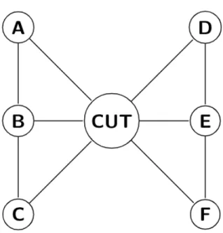
Definition 2.1.6. The block-cut tree, or metagraph of a graph G is the graph whose vertex set contains a vertex for each biconnected component ofGand for each cut vertex in G. The edge set of the block-cut tree contains an edge between each biconnected component and cut vertex belonging to that component (See Figure 2.3).
Figure 2.2: A graph divided into two biconnected components by a central cut vertex. Removing the cut vertex would disconnect the graph.
Figure 2.3: The metagraph of the graph in Figure 2.2. Note that CUT has its own vertex but is also included in both biconnected components, as cut vertices are part of both biconnected components that they divide.
Definition 2.1.7. A validcoloringof a graphG= (V, E) is an assignment of colors to each vertex in V such that no vertices v1, v2 share a color if {v1, v2}2E.A valid k-coloring of a graph G = (V, E) is a coloring of G that uses at most k di↵erent colors (See figure 1.1 on Page 2).
This thesis is concerned with a type of graph called coloring graphs. For every graph G and number of colors k, there is a coloring graph Ck(G) that encodes all
valid k-colorings of G. This notation is consistent with that used by other literature [3, 5, 6]. Ck(G) is defined as follows:
Definition 2.1.8. The k-coloring graph Ck(G) is the graph whose vertex set
contains all valid k-colorings of base graph G, with edges existing between two vertices if and only if the colorings represented by those vertices di↵er by the color of exactly one vertex in G(See Figure 1.2).
One property of coloring graphs that motivates some of our research questions is their high degree of symmetry. In order to understand what we mean by symmetry, we must define graph isomorphism and graph automorphism.
Definition 2.1.9. Graphs G and H are isomorphic if there exists a bijection be-tween their vertex sets f :V(G)!V(H) such that any edge {v1, v2}2E(G) exists
if and only if {f(v1), f(v2)}2E(H) (See Figure 2.4).
Informally, an automorphism of a graph is an isomorphism between that graph and itself. Definition 2.1.10 gives a more formal definition of automorphism.
Definition 2.1.10. Anautomorphism of a graphG is a permutation of its vertex set f : V(G) ! V(G) such that any edge {v1, v2} 2 E(G) exists if and only if {f(v1), f(v2)}2E(G).
Figure 2.4: An isomorphism between two graphs, where f(A) = 1, f(B) = 2, etc.
We observe that all coloring graphs have k! automorphisms. Say a graph is 3-colored using red, blue, and yellow. If the coloring is valid, all the red vertices may be swapped to blue, and all the blue vertices may be swapped to red. The result will still be a valid coloring. More generally, in a valid k-coloring, all vertices of color 0 may be swapped to a di↵erent color, then all vertices of color 1 may be swapped to any of the remaining colors, etc. Consequently, there exist k! versions of each valid coloring. Therefore, for any coloring graph Ck(G), there exist k! versions of each
vertex.
2.2 Related Work
Graph coloring is a commonly studied problem in theoretical computer science. Computers have assisted graph coloring research as far back as 1977 when Appel and Haken used computer software to prove the four-color theorem of planar graphs [2]. Previous research has been done seeking relationships between properties of a base graph and the connectivity of its coloring graph [3, 5, 6, 8]. One property that arises frequently is the chromatic number col of the base graph, defined as the minimum k needed for a valid k-coloring to exist. Cereceda et al showed in 2007
that ifk col(G) + 2, Ck(G) is connected [5]. Furthermore, Choo and MacGillivray
showed in 2010 that for k col(G) + 3, Ck(G) is Hamiltonian (a stronger case of
biconnectivity) [8].
We now show known algorithms that have been used previously in coloring and connectivity research. We begin by showing an existing algorithm to compute all possible colorings of a graph.
2.2.1 Dancing Links
In recent years, the standard method for many backtracking algorithms has been the ”Dancing Links” technique used by Donald Knuth in his famous Algorithm X [13]. The idea behind Dancing Links is to restore removed nodes from a doubly linked list in an efficient manner. This pseudocode:
node.left.right node.right node.right.left node.left
will remove a node from the list, while this pseudocode:
node.right.left node
node.left.right node
will insert the node back into the list in its original position. The use of Algorithm X proposed by Knuth was to solve exact-cover problems [13]. His algorithm encodes an exact-cover problem in a bit matrix where removing rows and columns represents covering elements. Algorithm X uses backtracking, and Knuth therefore used the Dancing Links technique to reinsert removed rows and columns back into the matrix. Both exact-cover and graph coloring are NP-complete problems [12], so Knuth’s algorithm can also be used to solve graph coloring. TheSage documentation website shows a method for reducing a graph coloring problem into an exact cover problem and setting up a matrix for Algorithm X [4].
In Section 3.1, we show a backtracking algorithm inspired by dancing links that stores the state of the algorithm in a single bitstring and performs all updates with only bit arithmetic.
2.2.2 Tarjan’s Algorithm for Finding Articulation Points
The current point of interest for coloring graph research at University of Rich-mond is biconnectivity. Our software was motivated by the desire to compute and visualize the metagraph of any coloring graph. To construct a metagraph we need to compute the coloring graph’s biconnected components and the cut vertices between them. There is a known algorithm by Robert Tarjan that identifies the cut vertices in a graph [10]. This section explains that algorithm. Section 4.1 details how we enhanced Tarjan’s algorithm also to compute biconnected components.
Tarjan’s algorithm is used to find cut vertices in a connected graph. For a disconnected graph, the algorithm can be run individually on every connected com-ponent. The algorithm uses depth first search to traverse a graph, tracking two pieces of information about each vertex:
• The depth of the vertex, or its distance from the root in the DFS tree.
• Thelowpoint of the vertex, defined as the minimum depth among the descendants of the vertex in the DFS tree and the neighbors of those descendants in G (with a vertex counting as one of its own descendants).
A vertex v is a cut vertex if it has a child with lowpoint greater than or equal to the depth of v. The root is a special case; it is a cut vertex if it has more than one child. Figure 2.5 shows Tarjan’s algorithm partway through execution on an example graph.
Pseudocode for the key recursive portion of Tarjan’s algorithm is shown in Algo-rithm 1. Tarjan’s algoAlgo-rithm is run on a graph with the visitedfield of every vertex
Figure 2.5: Tarjan’s algorithm partway through execution. The DFS traverses in alphabetical order. Edges already traversed are marked in red. Known cut vertices are marked in green. Ordered pairs show (depth, lowpoint).
set to false, the depthand lowpointfor every vertex set to null, and theparent for every vertex set to null. The algorithm iterates through a vertex’s neighbor list. If a neighbor has not been visited, we recursively call Tarjan’s on the neighbor. If the neighbor has already been visited, we use its depth to update our lowpoint. Note that this implementation does not create or output biconnected components. It only marks the cut vertices. We modify this algorithm in section 4.1 to take in a graph and output its metagraph.
Algorithm 1 Tarjans
Input: vertex v, depthd
1: visited[v] true
2: depth[v] d 3: lowpoint[v] d
4: childCount 0
5: isCutVertex false
6: for all neighbors n of v do 7: if not visited[n]then 8: parent[n] v 9: Tarjans(n,d+ 1)
10: childCount childCount + 1
11: if lowpoint[n] depth[v] then 12: isCutVertex true
13: end if
14: lowpoint[v] min (lowpoint[v], lowpoint[n]) 15: else if n6=parent[v] then
16: lowpoint[v] min (lowpoint[v], depth[n])
17: end if 18: end for
19: if (parent[v]6= null AND isCutVertex) or (parent[v] = null and childCount>1)
then
20: Output v as a cut vertex
21: end if
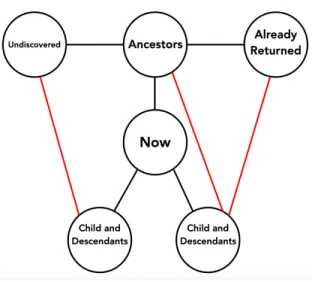
Figure 2.6: Tarjan’s algorithm partway through execution. At the current point in time, the algorithm is returning from a child to Now, with the lowpoint of the child being greater than or equal to the depth of Now. ThereforeNow will be marked as a cut vertex. By the rules of DFS, the red edges are all impossible.
Proof. Figure 2.6 shows Tarjan’s algorithm running on a graph. At the current point in time, the algorithm is returning from a child of the vertex Now. Say the lowpoint of the child is greater than or equal to the depth of Now. Tarjan’s algorithm will therefore mark Now as a cut vertex. If Now truly is a cut vertex, then none of the edges shown in red can exist, as each would form a cycle that would biconnect the vertices on both sides of Now. We now show that each of these red edges in figure 2.6 is impossible, proving that Now must be a cut vertex.
Case 1: Assume an edge exists from a descendant of Nowto an undiscovered vertex. If such an edge did exist, then the DFS would have traversed that edge before returning to Now. Therefore those vertices cannot be undiscovered, and we have reached a contradiction.
Case 2: Assume an edge exists from a descendant of Now to an ancestor of Now. If this edge exists, then a descandant of Now has a neighbor that is an ancestor of
Now. Therefore, the lowpoint of this descendant is at least as low as the depth of an ancestor of Now. The depth of an ancestor of Now is lower than the depth of Now. Therefore the lowpoint of the descendant is lower than the depth of now. We have reached a contradiction.
Case 3: Assume an edge exists from a descendant of Now to a vertex that has already returned. If such an edge exists, then DFS would already have processed the descendants of Now. If the descendants of now had already been processed, then they could not be descendants of Now. We have reached a contradiction.
At this point, we have established that any vertex marked as a cut vertex by Tarjan’s must be a cut vertex. Next, we must prove that no cut vertex in the graph will be missed. We prove this fact with the same construction. If Nowis a cut vertex, then none of the three red edges may exist. If none of the three red edges exist, then descendants of Now only have neighbors with depth greater than the depth of Now. Therefore the lowpoint of descendants of Now will have a lowpoint at least as great as the depth of Now. Therefore, Tarjan’s algorithm will mark Nowas a cut vertex.
3. COLORING GRAPH GENERATION
3.1 Computing Coloring Graph Vertices
The first step in generating a coloring graph is computing every possible coloring of the base graph. Our algorithm uses backtracking as the logical core with bit arithmetic as a mechanism. The goal of color generation is to output a list of integers where each integer is both the name and encoding of a valid coloring. Each encoding can be thought of as an integer in base-k where the ith digit of the integer tells the color of vertex vi. Because the encoding of a coloring is also the name of the
corresponding vertex in the coloring graph, the algorithms in this section frequently use the name of a vertex in the coloring graph as a number.
At a high level, our coloring algorithm iterates through the vertex list assigning colors until either all vertices are colored or a vertex is reached that has no legal col-ors. Beginning at depth 0, vertex 0 is assigned a color, then the depth is increased. At each depth, one vertex is assigned a color. If the vertex cannot be colored, the algorithm backtracks to the previous depth. For proper backtracking, the algorithm must track several things at each depth:
• Which colors can legally be assigned to a vertex at the current depth. This infor-mation is called the state of the algorithm.
• The current assignment of colors.
• The vertex that is trying to be colored at the current depth.
• The color most recently tested for legality at the current depth.
Each time the algorithm colors a vertex, it updates the state and assignment ac-cordingly. It then picks a new vertex to color. If the vertex cannot be colored, the algorithm will backtrack by reverting to the previous state and assignment. All of
Figure 3.1: A visual representation of how thestatebitstring is indexed for a graph with size V and k= 4. This same indexing is used for the assignment bitstring.
these processes are done with bit arithmetic.
The state is stored as a bitstring of length kv, where each bit corresponds to one potential vertex-color assignment (See Figure 3.1). The first bit represents the legality of vertex 0 being assigned color 0; the second bit represents the legality of vertex 0 being assigned color 1; etc until the last bit, which represents vertex v 1 being assigned colork 1. If we want to check whether vertexvimay be assigned color
kj, we use a command similar to state.test(vi * k + kj). This same indexing is
used for the assignment bitstring. Each bit in the assignment encodes whether that vertex-color combination has been chosen.
Pseudocode for finding all colorings is shown in Algorithm 2. At each depth, the algorithm tries to color a vertex, beginning with color 0. If color 0 is not allowed, it will try color 1, then 2, until k 1. If no color can be assigned, the algorithm will backtrack to the previous depth. Once the depth reaches |V|, the complete assignment is encoded as an integer and turned into a vertex in the coloring graph. This process continues until all possible colorings have been found. A few comments:
1. The method in line 1 computes a set of bitstrings that are used to update the state during the algorithm. These bitstrings are stored in the array referenced in line 16. This method is discussed later in this section.
2. The bit operations in line 2 produce a bitstring of entirely 1’s. The state at depth 0 must show that all vertices may be assigned any color.
3. The encode method in line 10 converts the assignment to an integer that can be interpreted in base-k. This integer is used as the ID for the vertex created in the coloring graph.
4. Because the state and assignment need to be stored at every depth, we use ar-rays that can be accessed using state[depth] orassignment[depth]. These arrays make progression and backtracking easy, since depth is stored as a vari-able that can be incremented to access the appropriate information. Note that the maximum depth of the algorithm is equal to the number of vertices in the base graph, so these arrays are statically sized.
5. The algorithm is written in a way that the vertices could be colored in any order. Line 18 ensures that the vertices will be colored in numerical order by their ID, but heuristics could be implemented here to choose vertices more wisely. This idea is discussed further in section 5.2.
These next few pages discuss the computeUpdateBitstrings helper method in Algorithm 2. The idea of this method is to precompute all possible bit arithmetic that may be necessary to update the state after assigning a color. Say we are trying to 3-color a graph with four vertices set up in a square.
0
2
1
3
Algorithm 2 Find All k-Colorings ofG
Input: GraphG= (V, E),int k
1: computeUpdateBitstrings() . This is shown on page 21.
2: state[0] (1⌧(k⇤size())) 1 3: assignment[0] 0 4: vertex[0] 0 5: color[0] -1 6: depth 0 7: while depth 0do 8: color[depth] color[depth] + 1
9: if depth = size() then . We have assigned a color to every vertex
10: cg.addVertex(encode(assignment[depth], k))
11: depth depth 1
12: else if color[depth] = k then .We have exhausted all colors for vertex[depth]
13: depth depth 1
14: else if state[depth].test(vertex[depth] * k + color[depth])then .We color vertex[depth] with color[depth] and update the graph
15: index vertex[depth] * k + color[depth]
16: state[depth+1] state[depth] & updateBitstrings[index]
17: assignment[depth + 1] assignment[depth] 18: assignment[depth + 1].set(index) 19: depth depth + 1 20: vertex[depth] depth 21: color[depth] -1 22: end if 23: end while
111 111 111 111.
Since we are allowing three colors, each set of three bits corresponds to one vertex. The first bit in a set shows whether that vertex can be assigned color 0. The second bit in a set shows whether that vertex can be assigned color 1. The third bit in a set shows whether that vertex can be assigned color 2. All bits are 1’s at the beginning because any vertex can be assigned any color. If vertex 0 is assigned color 0, the state must be updated to look like this:
111 110 110 000.
The entire block corresponding to vertex 0 has been zeroed out (vertex 0 is on the right, vertex 3 on the left), since none of those options will be chosen unless we backtrack and uncolor vertex 0. Furthermore, the blocks for vertices 1 and 2 both have had their first bit changed to 0. Because vertices 1 and 2 are neighbors of vertex 0, they can no longer be assigned color 0. But because they can still be assigned colors 1 or 2, the other two bits in both those blocks are still 1’s. Now, if we assign vertex 1 color 2, we need to update the state to look like this:
011 110 000 000.
The block for vertex 1 has been zeroed out, and vertex 3 has been disallowed from being color 2. Each vertex-color assignment disallows certain other assignments, and those assignments can be computed before coloring begins. No matter what the state of the algorithm may be, assigning vertex 1 color 2 will always update the state in the following manner:
state state AND 011 111 000 011.
This bitstring has 0’s in the exact locations that have just been disallowed. The goal of Algorithm 3 is to precompute similar bitstrings for any possible assignment. With this information, updating the state while coloring becomes easy. These bitstrings must have two properties:
Given a vertex v and a color c,
• All bits that correspond to v must be 0’s.
• All bits that correspond to neighbors of v receiving color cmust be 0’s.
Pseudocode for generating these bitstrings is shown in Algorithm 3. Note that this algorithm computes the negation of the bitstring we are looking for since the bit operations to do so are much simpler. The resulting bitstrings will be negated before they are used in Algorithm 2.
The algorithm generates two bitstrings for each vertex that can be combined to produce the final desired bitstring. It begins by computing the ”blockBits” for each vertex. The blockBits for a vertex v are a bitstring where all bits are 0’s except for the k consecutive bits that correspond to the possible colorings of vertex v. The blockBits for any vertex are easily generated by shifting a size k group of 1’s until they reach the appropriate location in the bitstring. Using the same example from above with vertex 1 being assigned color 2, the blockBits for that bitstring are the bits corresponding to vertex 1. The bitstring we eventually want is:
011 111 000 011.
The blockBits will look like this:
111 111 000 111.
The second bitstring generated for each vertex is the ”adjacencyBits.” The ad-jacency bits for a vertex v are a bitstring where all bits are 0’s except for the first bit in the blocks for neighbors of v. This bitstring can be generated by iterating through v’s neighbor list and adding temp ⌧ (name * k), where name is the ID for a neighbor. Using the same example, the adjacencyBits look like this:
110 111 110 110.
Vertex 1 is connected to vertex 0 and vertex 3, so we disallow those vertices from sharing a color with vertex 1. Note that 0’s signifying adjacency are in the slots for
color 0, not color 2. Whenv’s adjacencyBits are ORed with its block bits, we obtain the appropriate bitstring to update the state for v being assigned color 0. To obtain the bitstrings for other colors, we simply shift the 0’s in the adjacencyBits left before ORing. The bits will be shifted repeatedly for each color until color k.
Algorithm 3 Compute Update Bitstrings
Input: GraphG= (V, E),int k
1: vertices[0].blockBits (1 ⌧ k) - 1 2: for i 1 . . . vertices.size()do 3: vertices[i].blockBits (vertices[i-1].blockBits ⌧ k) 4: end for 5: temp 1 6: for i 0 . . . vertices.size()do 7: current vertices[i]
8: for all name 2 current.neighbors do
9: current.adjacencyBits current.adjacencyBits _(temp ⌧ (name * k)) 10: end for
11: current.adjacencyBits current.adjacencyBits _ (temp ⌧ (current.name * k)) 12: end for 13: for i 0 . . . vertices.size()do 14: current vertices[i] 15: temp current.adjacencyBits 16: for j 0. . . k do 17: updateBitstrings.add(temp OR current.blockBits) 18: temp = temp ⌧1 19: end for 20: end for
3.2 Computing Coloring Graph Edges
One of the primary concerns in coloring graph generation is storage. For all fore-seeable, practical research purposes, base graphs and metagraphs will be relatively small. However, coloring graphs grow exponentially with the size of the base graph.
The maximum size of Ck(G) is kv, where v is the size of G. Take a base graph with
15 vertices and 4 colors, and the maximum size of the coloring graph is over 1 billion. Consequently, we want coloring-vertex objects to store as little information as possi-ble. The primary storage concern is neighbor lists, since any vertex in this example could have (k 1)v = 45 neighbors. Unfortunately, Tarjan’s algorithm requires knowledge of a vertex’s neighbors since DFS is the core of the algorithm. There is a workaround to this issue that involves computing neighbors on the fly when Tarjan’s requires that information. Consequently, we never store the edge sets of coloring graphs. Rather, this section explains how we compute neighbors of vertices in the coloring graph on the fly.
It was mentioned in the previous section that a vertex’s name encodes the coloring it represents in base-k. A vertex named 2120 in base-3 would represent a coloring where vertex 0 is color 0, vertex 1 is color 2, vertex 2 is color 1, and vertex 3 is color 2. We can break this encoding down like so:
2120 = 2000 + 0100 + 0020 + 0000.
Each addend shows the color of one vertex. The base-10 addend for any vertex-color combination can be computed with color * (k ** v). We can take advantage of these addends to find the neighbors of a coloring-vertex. Say we wanted the neighbors of coloring-vertex 2120. We know that the neighbors are the coloring-vertices with exactly one di↵erent color. Because of our base-k encoding, we know that any neighbor will have an encoding with exactly one di↵erent digit. For example,
2121 is a neighbor of 2120. Thus, to iterate through the neighbor list of 2120, we need to iterate through every base-k number with exactly one di↵erent digit. If any of those numbers shows up in the vertex list for the coloring graph, we know it is a neighbor. This process is shown in Algorithm 4. The algorithm uses modular arithmetic to figure out what the encoding of a vertex would have been if it had one
di↵erent color. It then checks to see whether that encoding exists in the coloring graph. If the encoding exists, then it is returned, since it must be a neighbor. A few comments on Algorithm 4:
1. This method belongs to an object called ColoringVertexNeighborIterator. Each coloring-vertex stores its own iterator. The variables positionctr and
colorctrareinstance variables of the iterator. This way, the iterator can keep track of where to begin iteration every time Algorithm 4 is called.
2. precompexp is a precomputed, 2-D vector that stores the addends for every vertex-color combination. Using the arithmetic above,
precompexp[v][c] --> c * (k ** v)
3. The variablenameis the ID/encoding of the coloring-vertex calling the method.
This algorithm concludes our process for generating the coloring graph. To ana-lyze the connectivity of the coloring graph, we use Tarjan’s cut vertex algorithm [10] to generate the metagraph. Section 4 shows our implementation of that algorithm and the end result when viewed in our GUI.
Algorithm 4 Get Next Neighbor
Input: GraphG, int name
Iterator state variables: int positionctr, int colorctr
1: for positionctr positionctr. . . baseGraph.size() do 2: addend precompexp[positionctr][1]
3: curcol (name / addend) mod k
4: for colorctr colorctr. . . k do 5: if colorctr = curcol then
6: continue
7: end if
8: newcoloring name
9: newcoloring newcoloring - precompexp[positionctr][curcol]
10: newcoloring newcoloring + precompexp[positionctr][colorctr]
11: if vertices.contains(newcoloring) then 12: colorctr colorctr + 1 13: return newcoloring 14: end if 15: end for 16: colorctr 0 17: end for
4. METAGRAPH GENERATION
4.1 Modifying Tarjan’s Algorithm
We want to produce a metagraph that shows the biconnected components of a coloring graph and the cut vertices between them. The implementation of Tarjan’s algorithm in Section 2.2.2 fails to meet our goals in two ways. First, it only computes the cut vertices and not the biconnected components that they separate. Second, the recursive nature of the implementation is not sustainable on large coloring graphs. We modify Tarjan’s algorithm to fix both of these issues.
Pseudocode for our implementation is shown in Algorithm 5. The algorithm creates and outputs a metagraph consisting of metavertices. A metavertex is a bi-connected component of the input graph. It stores its own vertex list that includes any cut vertices in the component. Rather than contructing edges between bicon-nected components, we construct additional metavertex objects for each individual cut vertex and connect biconnected components through those cut vertices. Due to length, the pseudocode in Algorithm 5 leaves out some edge cases involving the root and disconnected input graphs. Below are some comments explaining the code.
1. Lines 2-14 follow the same traversal logic as Algorithm 1. But instead of recursively calling Tarjan’s on newly discovered vertices, we add the vertices to a list. The iterator current tracks which vertex in the list is being processed. Vertices in the list store their parent in the DFS tree, since the parent is not necessarily the previous vertex in the list.
2. Line 4 uses thegetNextNeighbor method explained in section 3.2.
vertex is discovered, we create a new metavertex and splice into it all the vertices from the current location in the vertex list to the end. The cut vertex itself must then be added to the metavertex since it will not be in the range (current, end). We do not want to remove the cut vertex from the vertex list yet since it will belong to another metavertex on the other side of the cut.
4. Details of Line 19: It is possible that some of the vertices that get spliced into a metavertex are cut vertices themselves. In this case, we need to add an edge from the new metavertex to each of these cut vertices. We accomplish these connections with the use of a stack. Each time we discover a cut vertex, we add it to a cut vertex stack. When a biconnected component is created, we examine all the cut vertices on the stack. If any of those cut vertices on the stack are contained in the new metavertex, an edge will be added.
4.2 The UI
Figure 4.1 shows the interface of the software that we created. In the top-left pane, the user may freely construct a base graph. After constructing a base graph and choosing a k value, clicking the “generate” button will begin construction and analysis of the coloring graph. The top-right pane shows the completed coloring graph with cut vertices marked in red. The bottom-left pane shows a block-cut tree, or metagraph, of the coloring graph. This metagraph is useful for connectivity analysis. Finally, the bottom-right pane shows what the o↵shoots in this graph look like, beginning with the cut vertex that separates them from the central component. Since some graphs have multiple polymorphic classes of o↵shoots, one o↵shoot from each polymorphic class will be displayed in this pane.
All graph classes and algorithms were written in C++. To ease distribution, we wrapped the graph library in SWIG to allow the code to be run in Python, then we
Algorithm 5 Modified Tarjans
Input: GraphG
1: mg new MetaGraph()
2: current random vertex ofG
3: while true do
4: child current.getNextNeighbor()
5: if child6= null and not visited[child] then 6: vertexList.push back(child)
7: current vertexList.end()
8: else
9: current.lowpoint min(current.lowpoint, child.depth) 10: if current.hasNextNeighbor() then
11: continue
12: end if
13: break if: current = root
14: parent.lowpoint min(parent.lowpoint, current.lowpoint)
15: if parent = root or current.lowpoint parent.depth then 16: foundCutVertex parent
17: MetaVertex mv mg.addVertex(foundCutVertex)
18: MetaVertex cutmv mg.addVertex(foundCutVertex)
19: mv.connect(all in range: cutVertexStack.top...foundCutVertex)
20: mv.connect(cutmv) 21: cutVertexStack.push(cutmv) 22: current foundCutVertex 23: else 24: current parent 25: end if 26: end if 27: end while 28: return mg
Figure 4.1: An example of coloring graph generation and analysis in the software. In the top-left, the user may construct a base graph. The top-right shows the coloring-graph. The bottom-left shows the metacoloring-graph. The bottom-right shows isomorphism classes of o↵shoots from the central component.
used Flask to allow the code to be run in a web browser. The graphs are visualized with the Javascript library Pyvis [1].
This UI was designed as a first attempt at coloring graph visualization. It has been useful for testing hypotheses and building intuition about coloring graph struc-ture. However, it is limited to small test cases since it displays the full coloring graph, and coloring graphs grow exponentially with the size of the base graph and number of colors. Section 5.1 explains potential improvements to the UI.
5. FUTURE DIRECTION
Our software is designed with current research goals in mind, and it has proved useful in testing our hypotheses. It has been particularly useful for finding coun-terexamples to hypotheses since scripts can be written to generate mass numbers of random graphs and test them for certain properties. However, several aspects of the software’s design may become outdated as research progresses. Section 5.1 explains some limitations of the software and how it may need to be reworked at a later date. Section 5.2 discusses potential improvements to the implementation of current algorithms.
5.1 Design Improvements
Coloring graph research is still in a primitive state. The majority of research and literature on the topic only examines coloring graphs where k 4. It is unclear how our hypotheses have been limited by our previous inability to compute larger coloring graphs. It is important to keep in mind that our software is tailored for current research questions. Its capabilities, therefore, are limited by our current understanding of coloring graphs. As research becomes more advanced, the interface may benefit from redesign. Seeing the full coloring graph is not normally useful since the sheer size of the central component overloads Pyvis. The coloring graph also does not inform our understanding of the connectivity any better than the metagraph.
We spend most of our time looking at the o↵shoots from the central component, as our current hypotheses involve the connective structures that arise in o↵shoots. For example, we have hypothesized that all o↵shoots from the central biconnected component of a coloring graph are subgraphs of hypercubes. We believe that this hypothesis will be much easier to prove or disprove if we can compute larger coloring
graphs. Particularly when our test cases become larger and we want to examine larger o↵shoots, we may no longer want to dedicate a pane to the coloring graph or the metagraph. Rather, we may want to write algorithms to analyze the colorings in o↵shoots and display that data instead.
5.2 Implementation Improvements
In addition to UI improvements, a number of improvements could be made to the implementation of existing algorithms. This section explains two improvements that we have discussed but not implemented.
One possible improvement would be expanding the scope of the bit arithmetic used for coloring-vertices. Algorithm 2 on page 18 uses a bitstring calledassignment
to track the current assignment of vertices. Once a valid assignment is reached, the bitstring is encoded as a number in base-k that is then used as the ID for a coloring-vertex.
It would likely be more time efficient not to use base-k encodings at all. The ID for a coloring-vertex could simply be the same bitstring generated by Algorithm 2. This change would save time not only while generating the coloring-vertices, but also while computing their neighbors. Section 3.2 explains how we need to precompute base-10 addends for every possible vertex-color combination to find the neighbors of a base-k encoded vertex. This process would be faster if the encodings were bitstrings since a candidate neighbor can be generated by flipping just two bits in the encoding. For example, say we have this base-4 encoding:
2 3 3 1 0.
The assignment bitstring would look like this (vertex 0 on the right):
0000 0010 1000 1000 0100
encoding would be this:
0000 0010 1000 1000 1000
By flipping two bits, we obtained a candidate neighbor. Using bitstrings for the ID’s of coloring-vertices is one way we could save time at the cost of the space needed to store bitstrings. Memory complexity was our primary concern when first designing our implementation of Tarjan’s algorithm, but recent profiling shows that Tarjan’s is the runtime bottleneck. On 1000 tests of base graphs with |V| = 8, k = 4, Tarjan’s takes around 9.14 times longer on average than computing the coloring graph. With
|V|= 11, k = 4, Tarjan’s takes around 7.57 times longer. It is possible that Tarjan’s will become relatively more efficient as test sizes increase; however, Tarjan’s runtime is linear in the size of the coloring graph, so it will scale exponentially with the size of the base graph. Using bit arithmetic to compute neighbors faster on the fly could greatly improve runtime.
Another possible improvement for coloring generation involves the order in which we color vertices. Currently, we color vertices in numerical order by their ID. But heuristics could be implemented here to improve the runtime. It is important to remember that a backtracking algorithm has a natural pruning e↵ect. If the algo-rithm realizes that a full coloring is impossible after coloring just three vertices, it will not test any more colorings that have those three vertices colored in the same way. Those colorings have all been pruned out of the search space. Because of this pruning e↵ect, the algorithm finishes the fastest when it fails early.
One common sense way to make the algorithm fail as early as possible is to color vertices in order of degree from highest to lowest. The idea is that vertices with lots of edges will eliminate the most options, causing the algorithm to fail sooner. This ordering is not proven to make significant runtime improvements; some research suggests that it may in fact worsen runtime on large graphs [9]. Furthermore, J¨org
Rothe showed in 2000 that coloring vertices in this order does not make it any easier to find the chromatic number of a graph [15]. We may implement this ordering in the future, but in addition, we propose that a preprocessing step would find the maximum sized clique in the base graph. Max-clique is an NP-hard problem [12], but base graphs are small enough that this preprocessing would still save time. Because all vertices in a clique need to be di↵erent colors, we could fix the colors of those vertices so that they are guaranteed not to conflict. Fixing these vertices would reduce the size of the search space by a factor of (k |max cliquek! |)!. Base graphs are relatively small, so the max-clique will frequently be big enough for that reduction to be significant. The changes we have described here would reduce runtime, albeit at the cost of space. We will need to test these changes to see how they a↵ect processing of larger graphs. The size of coloring graphs is the primary hindrance to the research that motivated our software. Future decisions must be made based on whether they improve processing of larger test cases.
REFERENCES
[1] Interactive network visualizations. https://pyvis.readthedocs.io/en/ latest/.
[2] K. Appel and W. Haken. Every planar map is four colorable. part i: Discharging.
Illinois J. Math., 21(3):429–490, 09 1977.
[3] P. Bonsma and L. Cereceda. Finding paths between graph colourings: Pspace-completeness and superpolynomial distances. Theoretical Computer Science, 410(50):5215 – 5226, 2009. Mathematical Foundations of Computer Science (MFCS 2007).
[4] T. Boothby. Graph coloring. http://doc.sagemath.org/html/en/reference/ graphs/sage/graphs/graph_coloring, 2008.
[5] L. Cereceda, J. [van den Heuvel], and M. Johnson. Connectedness of the graph of vertex-colourings. Discrete Mathematics, 308(5):913 – 919, 2008. Selected Papers from 20th British Combinatorial Conference.
[6] L. Cereceda, J. [van den Heuvel], and M. Johnson. Mixing 3-colourings in bi-partite graphs. European Journal of Combinatorics, 30(7):1593 – 1606, 2009. EuroComb’07: Combinatorics, Graph Theory and Applications.
[7] G. J. Chaitin. Register allocation spilling via graph coloring. SIGPLAN Not., 17(6):98–101, June 1982.
[8] K. Choo and G. MacGillivray. Gray code numbers for graphs. ARS MATHE-MATICA CONTEMPORANEA, 4(1):125–139, 2010.
[9] W. Hasenplaugh, T. Kaler, T. B. Schardl, and C. E. Leiserson. Ordering heuris-tics for parallel graph coloring. In Proceedings of the 26th ACM Symposium on
Parallelism in Algorithms and Architectures, SPAA ’14, page 166–177, New York, NY, USA, 2014. Association for Computing Machinery.
[10] J. Hopcroft and R. Tarjan. Algorithm 447: Efficient algorithms for graph ma-nipulation. Commun. ACM, 16(6):372–378, June 1973.
[11] T. Ito, E. D. Demaine, N. J. Harvey, C. H. Papadimitriou, M. Sideri, R. Ue-hara, and Y. Uno. On the complexity of reconfiguration problems. Theoretical Computer Science, 412(12):1054 – 1065, 2011.
[12] R. Karp. Reducibility among combinatorial problems. Complexity of Computer Computations, 40:85–103, 1972.
[13] D. Knuth. Dancing links. Millennial Perspectives in Computer Science, 1:187– 214, 2000.
[14] D. Marx. Graph coloring problems and their applications in scheduling. Periodica Polytechnica, Electrical Engineering, 48, 10 2003.
[15] J. Rothe. Heuristics versus completeness for graph coloring. Chicago Journal of Theoretical Computer Science, 2000(1), 2000.