University of Mississippi University of Mississippi
eGrove
eGrove
Electronic Theses and Dissertations Graduate School
2018
Multiobjective Reservoir Optimization Using Genetic Algorithm
Multiobjective Reservoir Optimization Using Genetic Algorithm
Seyma Tiryakioglu University of Mississippi
Follow this and additional works at: https://egrove.olemiss.edu/etd
Part of the Engineering Commons
Recommended Citation Recommended Citation
Tiryakioglu, Seyma, "Multiobjective Reservoir Optimization Using Genetic Algorithm" (2018). Electronic Theses and Dissertations. 435.
https://egrove.olemiss.edu/etd/435
This Dissertation is brought to you for free and open access by the Graduate School at eGrove. It has been accepted for inclusion in Electronic Theses and Dissertations by an authorized administrator of eGrove. For more information, please contact [email protected].
MULTIOBJECTIVE RESERVOIR OPTIMIZATION USING GENETIC ALGORITHM
A Thesis
presented in partial fulfillment of requirements for the degree of Master of Science
National Center for Computational Hydroscience and Engineering The University Of Mississippi
by
SEYMA SEHRIBAN TIRYAKIOGLU May 2018
Copyright © 2018 Seyma S Tiryakioglu All rights reserved
ABSTRACT
This thesis investigates the optimization of energy generation in a multipurpose reservoir. The objective functions and the constraints for the multiobjective optimization of reservoir operation for maximization of energy production involve the solution of a set of nonlinear equations governing pressure flow in penstock and turbine system and the hydropower generation. The hydropower generation also requires operational rules that define how the reservoir storage volume must be used at different storage levels. For these reasons, the present thesis uses genetic algorithm (GA) functions available in Matlab to perform the multiobjective optimization of hydropower energy production. Multiobjective optimization is based on two objective functions: maximization of total energy production over a specified number of years for which observed data is available, and maximization of annual firm energy production for individual years.
Two separate Matlab codes using different hydropower generation algorithms were written for multiobjective optimization using GA. One of the two Matlab codes disregards the operation of individual turbines when allocating the storage volumes for firm energy and secondary energy and uses a nominal head loss due to the friction. The second Matlab code allocates the storage volumes for firm energy and secondary energy by considering hydropower production by individual turbines and the true head losses for each turbine.
In addition to these two Matlab codes for multiobjective GA optimization of the reservoir operation, a third Matlab code was also written to calculate the energy production using a
These three Matlab codes were applied to calculate the hydroelectric power generation in a multipurpose reservoir. The reservoir operation strategies determined using GA, with and without the consideration of the operation of individual turbines, were then compared with the those obtained using the rule-based traditional method and the results of the original worksheet analysis provided by the State Water Works (DSI) of Turkey. Using prescribed operational policy and rule-set, this study shows that compared to traditional and DSI results, operations conducted using genetic algorithms produce both higher firm energy and a greater total energy production. Further, these results are found to be accurate over a period of 30 years.
LIST OF ABBREVIATIONS
GA Genetic Algorithm
ICOLD International Congress on Large Dams
DSI Devlet Su Isleri (State Water Works) of Turkey GAT Genetic Algorithm Toolbox
ACKNOWLEDGMENTS
I would like to express my deepest appreciation to my advisor, Dr. Mustafa S. Altinakar and my committee members, Drs. Bahram Alidaee, Yafei Jia, and Vijay Ramalingam. In addition, I thank Nazmi Kagnicioglu, Veysel Yildiz and Murat Yakut who have helped me and cooperated with me during my project work.
Finally, I am extremely thankful to my friends Luc Rebillout, Nazim Sahin and my family for their generous support.
TABLE OF CONTENTS
ABSTRACT ... ii
LIST OF ABBREVIATIONS ... iv
ACKNOWLEDGMENTS ... v
LIST OF TABLES ... viii
LIST OF FIGURES ... ix
1. INTRODUCTION ... 1
1.1. Statement of the Problem ... 4
1.2. Test Case for Evaluating Developed Methods ... 7
2. OPTIMIZATION OF RESERVOIR OPERATION ... 10
2.1. General Information ... 10
2.2. Nonlinear Optimization and Genetic Algorithm Technique ... 11
2.3. Genetic Algorithm ... 13
2.3.1. Selection (Reproduction) ... 14
2.3.2. Crossover ... 15
2.3.3. Mutation ... 17
2.4. Literature Survey on the Use of Genetic Algorithms for Optimization of Reservoir Operations ... 18
3. GENETIC ALGORITHM OPTIMIZATION OF RESERVOIR OPERATIONS USING
MATLAB ... 21
3.1. Genetic Algorithm Programming Using Matlab ... 21
3.2. Formulation of the Multiobjective Optimization Problem in Matlab ... 25
3.3. Description of the Matlab Code: A Study Case ... 30
3.4. The Concept of Energy Generation at a Dam and the Formulation of Hydropower Generation ... 34
3.5. Final Considerations for the Matlab Code with Genetic Algorithm ... 39
4. RESERVOIR OPERATION USING RULE-BASED TRADITIONAL METHOD (CODE03) ... 43
5. CASE STUDY: KAYRAKTEPE DAM IN TURKEY ... 48
6. DISCUSSION OF RESULTS AND CONCLUSIONS ... 57
6.1. Comparison of Results of CODE01 with Operational Data from the DSI ... 59
6.2. Comparison of Results of CODE02 with CODE03 ... 65
6.3. Sensitivity of the Optimal Results to the Parameters of Genetic Algorithm ... 69
6.4. Conclusion ... 70
7. FUTURE WORK ... 76
REFERENCES ... 78
LIST OF TABLES
Table 1 List of input variables for the Matlab genetic algorithm code. ... 30 Table 2 Characteristics of the Kayraktepe Dam Project. ... 50
LIST OF FIGURES
Figure 1 Storage allocation zones of a reservoir. ... 4
Figure 2 Illustration of reservoir operation. ... 6
Figure 3 Concept of solution space. ... 11
Figure 4 Illustration of global and local maximum points in a nonlinear problem. ... 12
Figure 5 Flowchart of genetic algorithm. ... 14
Figure 6 Tournament method for “Selection” step. ... 15
Figure 7 Illustrations one point, two points, and uniform crossover methods. ... 17
Figure 8 The interface of Genetic Algorithm Toolbox (GAT) in Matlab ... 22
Figure 9 Plot options for the genetic algorithm in Matlab. ... 24
Figure 10 Flowchart of the genetic-algorithm Matlab code for the optimization of energy generation. ... 33
Figure 11 Hydraulics of energy generation at a dam. ... 34
Figure 12 Friction coefficient graphs for Haaland (1983) and Altshul (1952). ... 38
Figure 13 Illustration of reservoir zones for the rule-based traditional method. ... 43
Figure 14 Illustration of storage volume allocation for the case “a.1”. ... 45
Figure 15 Illustration of storage volume allocation for the case “a.2”. ... 45
Figure 16 Illustration of storage volume allocation for the case “a.3”. ... 46
Figure 18 Location of dams and their operating status Red: under construction (Bagbasi, Bozkir, Ermenek), Yellow: in the project development phase (Mut, Kayraktepe), Green: already
operating dam (Gezende). ... 48
Figure 19 Monthly irrigation volume needs of the agricultural sector. ... 49
Figure 20 The stream gaging and meteorological gaging stations. ... 51
Figure 21 Monthly precipitation rates. ... 52
Figure 22 Monthly average temperatures. ... 52
Figure 23 Monthly evaporation volumes. ... 52
Figure 24 Time series of monthly inflow volume into the Kayraktepe Reservoir. ... 53
Figure 25 Time series of monthly inflow (𝐼) and potential energy (𝑃𝐸𝑉) volumes. ... 54
Figure 26 Duration curve for monthly potential energy volume (𝑃𝐸𝑉). ... 55
Figure 27 Elevation-volume and elevation area curves for Kayraktepe Reservoir. ... 56
Figure 28 Modeling of the Kayraktepe Project... 58
Figure 29 Comparison of end of the month storage volumes obtained from optimization using CODE01 with the results provided by the DSI. ... 61
Figure 30 Comparison of end of the monthly energy production obtained from optimization using CODE01 with the results provided by the DSI. ... 62
Figure 31 Pareto front obtained using Matlab for CODE01 ... 63
Figure 32 Comparison of the annual total energy production obtained from optimization using CODE01 with the results provided by the DSI. ... 64
Figure 33 Comparison of the annual firm energy production obtained from optimization using CODE01 with the results provided by the DSI. ... 65
Figure 34 Comparison of end of the month storage volumes obtained with CODE02
(optimization by considering individual turbines) and CODE03 (rule-based traditional method). ... 66 Figure 35 Comparison of monthly energy production obtained with CODE02 (optimization by considering individual turbines) and CODE03 (rule-based traditional method). ... 66 Figure 36 Pareto front obtained using Matlab for CODE02 ... 67 Figure 37 Comparison of the annual total energy production obtained with CODE02
(optimization by considering individual turbines) and CODE03 (rule-based traditional method) ... 68 Figure 38 Comparison of the annual firm energy production obtained with CODE02
(optimization by considering individual turbines) and CODE03 (rule-based traditional method). ... 68 Figure 39 Efficiency curve for Francis Turbine ... 77
1. INTRODUCTION
One of the topics covered by applied mathematics is mathematical optimization.
Although various mathematical optimization problems have been studied earlier, the beginnings of modern mathematical optimization can be traced back to the development and formalization of calculus, and variational calculus by Gottfried Wilhelm (von) Leibniz and Sir Isaac Newton [1]. Since then, mathematical optimization methods have been extensively studied and developed by numerous mathematicians and scientists. The methods of mathematical optimization have been used to solve problems in numerous areas of science and engineering
One of the areas where optimization has been extensively used is the optimal use of water resources and optimal design of water storage structures, such as large dams. Schardong [2] used a multiobjective differential evolution algorithm (MODE) for optimization of a multiobjective reservoir system operation and compared it with genetic algorithm NSGA-II using some test cases. Afsharian Zadeh [3] used particle swarm optimization (PSO) for reliability based optimal design and operation of a cascading hydropower reservoir systems by formulating the
maximization of firm energy production while controlling the reliability level of hydroenergy production as a mixed integer nonlinear program (MINLP). Trezos [4] studied the planning of hydropower production of hydroelectric facility in Southern California using an integer
programming (IP) approach. Heydari [5] studied optimization of 5 dams in series on the Karun River and the Dez Dam parallel to those five by formulating the optimization problem as a matrix structure for multiobjective optimization of water supply and energy
production. Mujumdar and Nirmala [6] presented the development of an operating policy model for hydropower generation in a multi reservoir system using a Bayesian stochastic optimization model that considers uncertainties in both forecast uncertainty and inflow uncertainty. Qi et al. [7] presented the multiobjective optimization of hydropower generation in flood control operation using evolutionary algorithms which take into account preferences of the decision maker. Brown et al. [8] provides a short summary of the past efforts and discusses the future directions for water resources system analysis.
The water control structures, such as dams are built to provide a variety of services [6], which may include water supply for irrigation, drinking, and industrial use, flood control, fire protection, hydroelectric energy generation, and recreation, etc. Thousands of structures have been built around the world to address the specific needs of a region or a country. ICOLD (International Congress on Large Dams) has records of 57,835 large dams (with a dam height greater than 15m) in 96 countries [10]. China occupies the first position with 23,842 large dams followed by the United States of America with 9,265 large dams. Turkey occupies the 10th rank with 972 large dams. These structures are generally built at very high costs. Therefore, it is normal to expect that they would be operated in a manner to achieve maximum efficiency to fully meet the specific purposes for which they were designed.
Reservoirs are operated for flood control, navigation, hydroelectric power, municipal and industrial water supply, irrigation, water quality management, recreation, erosion and sediment control, fish and wildlife enhancement [11]. When a dam is being constructed, one or more of the above are selected as the goals. Often, these goals are ranked as primary, secondary and tertiary goals, etc.
The number of goals to be optimized when optimizing the operation of the reservoir determines whether the process is called single or multi-objective optimization. If there is a single goal to achieve (which is expressed as a mathematical function, called an objective function, to be maximized or minimized), the problem is a single objective optimization problem. The single objective optimization aims to find the best operational strategy for a reservoir by maximizing or minimizing this objective function subject to a set of constraints, which may be physical constraints or operational policy constraints.
Multi-objective optimization seeks to optimize multiple objective functions
simultaneously. These multiple objective functions may express conflicting goals. Thus, the multiobjective optimization leads to an optimal compromise, whereby the simultaneous
optimization of all the objectives does not necessarily lead to the optimal value of all individual objectives. In fact, there the multiobjective solution may lead to several optimal solutions. These solutions are gathered in a region known as Pareto Optimal [12]. The Pareto Optimal is a
collective optimal, or a set of nondominant solutions [2], in which none of the objective functions can be further improved without worsening the value of at least one other objective function. Pareto front represent different combinations of tradeoffs between the multiple objectives of the optimization problem [2]. Since the majority of large dams in the world are designed to meet more than one need, such as the combination of flood control and energy production, their operation involves multiobjective optimization.
Single and multi-objective optimization forms can be mathematically written as follows: Consider the vector of n control variables given below:
X
⃗⃗ = [𝑥1, 𝑥2, … , 𝑥𝑖, … , 𝑥𝑛−1, 𝑥𝑛] 𝑤ℎ𝑒𝑟𝑒 𝑥𝑖 ∈ 𝑅𝑛 (1) Multi Objective Optimization problem states that:
Maximize or Minimize: M⃗⃗⃗ (𝐹𝑗(X⃗⃗ )) = M⃗⃗⃗ (𝐹1(X⃗⃗ ), 𝐹2(X⃗⃗ ), … , 𝐹𝐽(X⃗⃗ ) ) 𝑤ℎ𝑒𝑟𝑒 𝑗 = 1, … , 𝐽 𝑆𝑢𝑏𝑗𝑒𝑐𝑡 𝑡𝑜 gk(𝑥1, 𝑥2, … 𝑥𝑛−1, 𝑥𝑛) ≤ 0 k = 1, 2, … , m
hℓ(𝑥1, 𝑥2, … 𝑥𝑛−1, 𝑥𝑛) = 0 ℓ = 1,2, … , r
(2)
where x ∈ Rn is a vector of n decision variables, 𝐹𝑗(X⃗⃗ ) are the objective functions, gk(X⃗⃗ ) are the inequality constraints, hℓ(X⃗⃗ ) are the equality constraints. If 𝐽, i.e. the number of objective
functions,is equal to one, the optimization problem is becomes a single objective optimization
1.1. Statement of the Problem
This research considers the multiobjective optimization of a multipurpose reservoir, which is designed to provide irrigation water, flood protection and energy production. Input data for the test case considered in this thesis includes monthly volumes of inflow, evaporation, and required volumes for irrigation release to downstream for a period of thirty years.
Figure 1 Storage allocation zones of a reservoir.
Reservoir storage is divided into four storage zones (Figure 1). Dead storage, which is also called inactive storage zone, is used for sediment storage. Located above the dead storage zone, active storage zone is divided into two subzones. The lower part is the buffer zone and the
upper part is the main active storage zone. The buffer zone may suffer from water quality problems. The buffer zone may have sediment particles within the storage, which reduces the water quality for reservoir operation. Therefore this zone is not preferred to use for reservoir operation. The main active storage zone is generally the preferred zone for reservoir operation. The flood control storage is where the excess water is stored in the reservoir to protect of the downstream from floods. Induced surcharge zone is the section, which is used for exceptional peak flows. Active reservoir storage is used for reservoir operation.
Reservoir operation concerns decision making with regard to the amounts of storage volume to be allocated and used for different purposes, such as irrigation, hydropower
generation, etc. Starting with an initial water storage volume of 𝑆𝑡 (in hm3) at the beginning of the month 𝑡, the storage at the end of the month 𝑆𝑒𝑛𝑑 (or 𝑆𝑡+1) is calculated taking into inflow volume, 𝐼, and outflow volume, 𝑂, using the mass (or volume) conservation equation given by Eq (3), which can be recursively applied for all months from 1 to 𝑇:
𝑆𝑒𝑛𝑑 = 𝑆𝑡+1= 𝑆𝑡+ 𝐼 − 𝑂 𝑡 = 1 … 𝑇 (3)
In this recursive equation, the end of the month volume for the month 𝑡, i.e. 𝑆𝑒𝑛𝑑 (or 𝑆𝑡+1), becomes the initial storage volume for the month 𝑡 + 1.
The volume of water entering the reservoir is defined as inflow volume, which includes the sum of runoff due to rainfall and snowmelt, and the water released from any upstream reservoirs. The outflow volume includes losses due to evaporation, releases for irrigation,
drinking water supply, environmental minimum water (the amount of water released each month to support and maintain the local ecosystem), and energy water (passing through turbines to
generate hydroelectric energy). In his research, only evaporation, irrigation and energy water volumes are considered as outflow (Figure 2).
Figure 2 Illustration of reservoir operation.
The present thesis seeks to optimize the hydroelectric energy production using two objective functions:
1. Maximize the total energy production over a period of specified number of year for which the data is available, and
2. Maximize the firm energy production for all individual years of the specified period.
Firm energy is defined as the amount of guaranteed hydroelectric energy produced continuously throughout the year. Since there are two objectives, a multi-objective optimization method is to be used.
The numerical solution of the reservoir routing equation and the calculation of friction losses in the penstocks involved in the computation of the objective functions are complex and nonlinear. Therefore, it was decided to use genetic algorithm techniques that are already available as functions in the Global Optimization Tool of the Matlab software.
Two separate Matlab codes were written for multiobjective optimization of the reservoir operation for hydroelectric energy production using different algorithms for calculating the energy production from an allocated storage volume. These alternative algorithms for hydroelectric energy production are as follows:
1. The algorithm for the allocation of volumes for firm energy and secondary energy or the production of the hydroelectric energy does not consider the operation of individual turbines. The hydroelectric energy generation is computed using a constant nominal head loss value irrespective of the turbine discharge. This code will be referred to as CODE01 from hereon.
2. The algorithm for the allocation of volumes for firm energy and secondary energy and the production of the hydroelectric energy take into account the number of turbines, their characteristics, and the distribution of allocated firm and secondary energy volumes between the individual turbines according to a specified operational policy. For each turbine, the energy produced is calculated by considering the true friction head loss computed based on the turbine discharge and the penstock characteristics. This code will be referred to as CODE02 from hereon.
A third Matlab code, which will be called CODE03 from hereon, was also written to compute the firm and secondary hydroelectric energy generation using a traditional rule-based method to allocate the volumes for firm and secondary energy production. This Matlab code also considers the energy production by individual turbines based on the partition of the volumes allocated for firm and secondary energy and the corresponding friction head losses.
Kayraktepe Dam located in southern Turkey near Mediterranean coast was selected as the test case for this thesis study. Revised planning report and various other data concerning
Kayraktepe Dam were kindly provided by the State Water Works Turkey (DSI). Along with the reports and data, the DSI also provided a spreadsheet of reservoir operation study for the
computation of the projected hydroelectric energy production, which is composed of firm energy and secondary energy, during a period of 30 years. These computations were carried out within the framework of the revised planning study, which considered the technical and economic feasibility of the irrigation of an area of 7,425 ha using pressure pipe flow and the generation of the hydroelectric power.
The worksheet included monthly volumes of inflow, losses due to evaporation, and various outflows (such as irrigation, drinking, environmental and energy water) for a 30-year (360 months) period extending from October 1984 to September 2013.
The three Matlab codes (CODE01, CODE02, and CODE03) were applied to the test case of Kayraktepe Dam. It is important to note that Kayraktepe Dam and reservoir is a multipurpose facility, whose primary purposes are flood protection and irrigation. Energy production is the secondary purpose.
The two Matlab codes with genetic algorithm optimization (CODE01 and CODE02) in the present study, however, focus on the maximization of the annual firm and total hydroelectric energy production. The third code (CODE03) applies a rule based traditional method to allocate the energy volume, which considers the operation of the individual turbines. For all thee Matlab codes, the monthly volumes required for the irrigation are treated as known time series, which is given as input to the program together with the know time series of losses through evaporation and leakage. All three codes receive these time series as input and accommodate them as outflow
volumes to be satisfied. The use of the remaining available storage volume is then optimized for energy production by maximizing the total energy production over the entire period of study and the individual annual firm-energy production amounts.
This thesis divided into seven chapters. The first chapter presents statement of problem and explains the purpose of the study. The second chapter explains the general information about optimization, genetic algorithm and compiles the literature sources for current study. The
optimization model, problem formulation and Matlab programming for genetic algorithm are explained in Chapter 3. Traditional method for reservoir operation is defined in Chapter 4. Chapter 5 presents a case of study with the problem assumptions and input variables for energy optimization. The sixth chapter on the discussion of results and conclusions presents the results of the energy production amounts obtained using the three Matlab codes and compare them with the original energy production calculations. The last chapter discusses the future work.
2. OPTIMIZATION OF RESERVOIR OPERATION
Various optimization techniques have been used for multiobjective reservoir operation. One of the techniques that can be used for solving non-linear multiobjective reservoir
optimization problems is the genetic algorithm. In this study, the genetic algorithm will be used for the nonlinear reservoir optimization problem in which monthly total energy production and firm energy maximization are performed. This chapter provides some general information about multiobjective optimization, genetic algorithm technique, and highlights some of the previous work related to the topic of this thesis.
2.1. General Information
The modeling of a multiobjective optimization problem for a multipurpose reservoir, such as the one considered in the present thesis, requires identification of the decision or control variable vector X⃗⃗ , the vector of objective functions M⃗⃗⃗ (𝐹𝑗(X⃗⃗ )), in which individual objective functions are defined based on the vector X⃗⃗ , and the set of constraints, which can be inequality constraints gk(𝑥1, 𝑥2, … 𝑥𝑛−1, 𝑥𝑛), or equality constraints hℓ(𝑥1, 𝑥2, … 𝑥𝑛−1, 𝑥𝑛), referring to Eq.(2).
Monthly reservoir storage volumes released for energy production (the total monthly volume for firm energy and secondary energy) are chosen as decision variables. The constraints impose lower and upper bounds for the values of the decision variables based on the discharge characteristics of the turbines. In addition, it is required that the reservoir is operated between
specified limits, and the mass conservation is imposed in the form of reservoir routing equation, see Eq. (3) which expresses the conservation of storage volume (water is considered
incompressible). Other constraints and/or rules are also imposed on how the turbines should be operated in CODE02) and CODE03.
Multiobjective optimization may produce multiple feasible solutions, within the feasible region that satisfies the constraints. These multiple feasible solutions do not necessarily
maximize all individual objectives (Figure 3).
Figure 3 Concept of solution space.
2.2. Nonlinear Optimization and Genetic Algorithm Technique
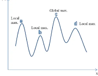
In linear programming, the optimal solution, which both local and global, is located at the vertices of the feasible region. The situation is different for nonlinear programming. Nonlinear problem may be more than one local maximum and minimum point. Referring to Figure 4, the function 𝑧 = 𝑓(𝑥) has multiple local maximum points, which are marked as “a”, “b”, “c” and “d”. However, the global maximum is located at point “c”.
Nonlinear and linear optimization problems can be formulated as constrained or
unconstrained. In constrained optimization formulation, constraints are defined for the decision variables and/or the objective functions. Unconstrained optimization problems incorporate interior [9] penalty functions into the objective function to force the results into the feasible region. Ideally, the penalty function becomes active when a chromosome is not satisfying the objective functions to guide the chromosome into the feasible region. However, for
multiobjective problems with multiple constraints defining the right form of penalty function may pose a serious challenge in itself.
Figure 4 Illustration of global and local maximum points in a nonlinear problem.
Optimization problems related to water resources are complex and nonlinear [2]. There is a nonlinear relationship between the components to be used for optimization. In this case,
nonlinear models may be preferred or optimization may be performed by using the linearization method. For example, when energy production is calculated, the relationship between released volume and the head loss is not linear.
2.3. Genetic Algorithm
GA is evaluated as a robust, efficient and quickly converged algorithm, and does not appear to cause any significant change in the results of program re-running. In this study, GA is preferred because of the high percentage of success in constrained, multidimensional and nonlinear problems.
The genetic algorithm was first described by the Holland [13] and later developed by Goldberg [14] and Michalewicz [15]. It is based on natural selection and natural evolution. Goldberg explains the structures that differentiate genetic algorithm from other algorithms with the following four approaches [14].
GAs do not work with parameters themselves but rather with the group created by coding the parameters.
GAs focus on the whole set of points rather than limiting their search to a single point. The information that GAs use is based on objective function, rather than auxiliary
knowledge such as derivatives.
GAs prefer probabilistic transition rules to deterministic rules.
The genetic algorithm makes a global search and it is population based. While the potential good solutions survive in the genetic algorithm, other solutions are removed from the population. The convenient solutions are determined according to the objective function, which is also called a fitness function. Crossovers and mutations operators of genetic algorithm method are used to create new generations.
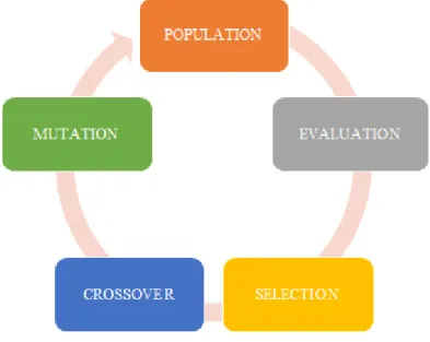
Figure 5 Flowchart of genetic algorithm.
In the genetic algorithm, each candidate solution is called a chromosome. The set of all candidate solutions is called the population. The population size is a parameter that defines the number of candidate solutions. As the population grows from generation to generation, poor solutions tend to disappear and good solutions tend to produce better solutions. Firstly, the initial population is randomly generated considering problem constraints. The value that determines how good a chromosome is for an optimal solution is called a fitness value. In the GA, the fitness value of the solution increases its chances of being selected for mutation and crossover process to create a new population. Figure 5 shows the main steps of the genetic algorithm. These steps “Selection”, “Crossover”, and “Mutation” are briefly discussed in the following subsections.
2.3.1. Selection (Reproduction)
To create a new generation, the chromosomes with high fitness rates are selected as parents. This process is called "selection". The selection of individuals is random process but fitter individuals have high probability from the other chromosomes. There are many selection methods such as the roulette wheel, tournament, and rank selection.
In the roulette wheel method, the probabilities of selection for chromosomes are proportional to the fitness values.
For the rank selection method, the choice of the parents depends on the rank of the individuals, but sorting is not related to fitness values.
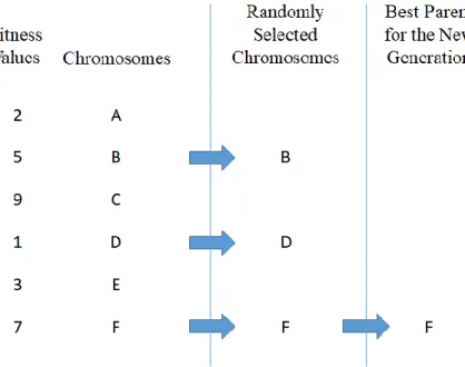
In this thesis, the “Tournament” method is preferred. To apply the tournament selection method, a certain number of individuals are randomly selected from the population and selection is made among these individuals by taking into account their fitness values Figure 6 schematically illustrates how the tournament method works.
Figure 6 Tournament method for “Selection” step.
2.3.2. Crossover
The crossover is the process of creating a new child from two selected parents. The purpose of crossover is to create a better generation by swapping genes from the parents who are selected in the first step. There is not a new generation until the crossover step is completed.
After swapping genes among the parents, a new and “better” generation is created. The creation of a better generation continues until the desired result is achieved. The criterion that determines whether there is a crossover between selected pairs is the crossover probability. Crossover probability is generally between 0.5 and 1. There is a wide range of crossover methods such as one point crossover, two point crossovers, uniform crossover, and intermediate crossover.
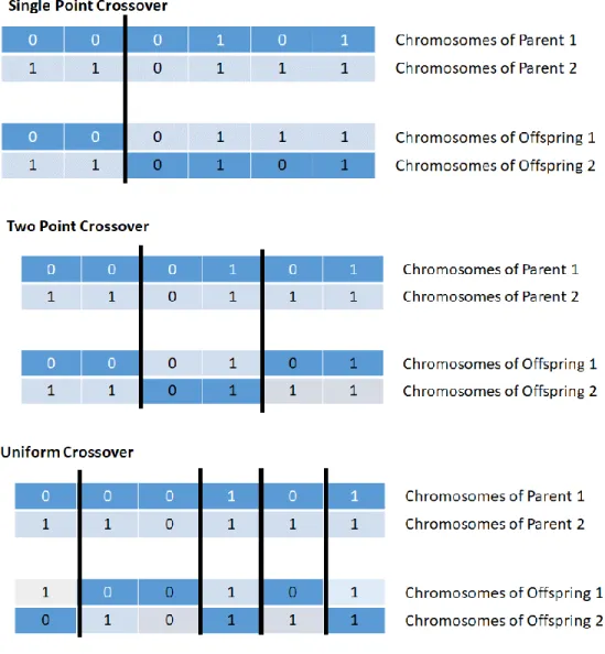
Figure 7, illustrates how the first three methods are applied. One point method randomly selects a single location in the gene sequence of both parents. The selected location is shown by a thick line in the figure. The genes of the parents to the left and right side of the selected location are swapped to create two offsprings. A similar procedure is use for the two point crossover with the difference that two locations are selected in the gene sequence for swapping the genes of two parents. In the uniform crossover method, instead of swapping blocks of genes, the decision to swap or not the genes is decided at the individual gene level based on a probability value, which is generally selected as 0.5.
In the present thesis, the intermediate cross over method is used. The explanations for this method will be provided in Chapter 1.
Figure 7 Illustrations one point, two points, and uniform crossover methods.
2.3.3. Mutation
After a certain period of new generation production, chromosomes in the next generation may repeat each other. This may lead to a decrease in the genetic diversity of new populations. The aim of the mutation is to preserve the genetic diversity. The probability of mutation is the operator that determines whether or not mutations will be made on genes. The mutation
probability usually takes small values. If this value is 100 %, all the chromosomes change, while if it is 0 %, the chromosomes remain the same.
2.4. Literature Survey on the Use of Genetic Algorithms for Optimization of Reservoir Operations
Traditional methods do not always offer the optimal solution for reservoir operation. The genetic algorithm is considered a robust and reliable technique for optimization of reservoir operation for single or multiple objectives. Numerous optimization problems for single and multi-reservoirs have been studied in the past using this algorithm. In these studies, several topics such as optimizing energy production, meeting irrigation and drinking water needs; providing ecological, environmental and socio-economic benefits; flood control and so on have been handled using the genetic algorithm.
Esat and Hall have conducted research to show the applicability of the genetic algorithm in multipurpose reservoirs [16]. Maximization of energy production and irrigation water was used as objective functions in this study. Capacity of reservoir release and storage were used as constraints. In this work, the adequacy of the genetic algorithm for water resources systems is demonstrated by comparing with other techniques. Oliveira and Loucks [17] evaluated the operating rules for multi-reservoir systems using genetic algorithm. The performance of the genetic algorithm was sufficient and practicable for different scenarios and problems in their studies. Another optimization research with genetic algorithms was published by Wardlaw and Sharif [18]. Previously published results, which were solved with dynamic programming for the same reservoir problem, were compared with results from the genetic algorithm in this study. The results of the genetic algorithm were evaluated and were determined to be robust and applicable even in complex systems. Optimization studies by genetic algorithm for three reservoirs in the Colorado River Storage Project were implemented by Hincal [19]. Actual operation data and the operation data resulting from the optimization study were compared. The
results showed that the genetic algorithm is competitive and constitutes a robust alternative to other optimization techniques. The studies made for the reservoir optimization with genetic algorithm have been done by using different coding methods throughout the years. Researchers have attempted to obtain optimal solutions using their own software codes or solvers provided by software packages.
Matlab is one of the software programs that offer solvers for different optimization methods used in engineering studies, including tools for the genetic algorithm. There are two solvers for the genetic algorithm, one for single objective optimization and the other for multiobjective optimization.
The genetic algorithm toolbox (GAT) can be used for both multi objective and single objective problems. The applicability of these solvers for reservoir optimization has been tested by various researchers. Hashemi et al. [20] studied reservoir optimization using GAT for different inflow probabilities. The downstream water needs were provided by regulating the reservoir volume balance for different scenarios. GAT gave fast and reasonable results. Another work that is optimized using GAT is by Devisree and Nowshaj [21]. This work was done to maximize the annual amounts of energy as well as irrigation water. The obtained results are compared with the results obtained with the linear programming solution. It was observed that the results were reasonably close to each other and satisfactory. In these studies, models are designed for a period one year, for which they provided good results.
The efficiency of the genetic algorithm has been tested for long periods (different flow scenarios). Research in this area was made by Yousif H. Al Ageeli, Lee and Aziz [22]. Energy generation was simulated for reservoir operation by using traditional method, and he compared it with results obtained by using a single objective genetic algorithm. Their aim is to maximize the
annual electricity generated. In addition, the inclusion and non-inclusion of precipitation and evaporation in optimization were compared by them. They concluded that in the scenario, which includes precipitation and evaporation, 65% more energy was produced and genetic algorithm was successful in different scenarios.
Considering all this, in this thesis, we will optimize the energy production of reservoir by using structural data, inflows and other necessary releases, which are available for a period of thirty years for the selected test case in Turkey. The purpose of this research is to evaluate the applicability and efficiency of the genetic algorithm for the problem of maximizing firm energy and annual energy production. The results obtained using genetic algorithm are then compared with both traditional ruled based reservoir operation results and the original calculations performed by an engineering company, which provided by the curtesy of DSI.
3. GENETIC ALGORITHM OPTIMIZATION OF RESERVOIR OPERATIONS USING MATLAB
Global Optimization Toolbox of Matlab provides a series of solvers to solve different types optimization problems (linear, quadratic, integer, and nonlinear) by maximizing or
minimizing one or more objective functions under defined constraints. One of these solvers is the genetic algorithm. In Chapter 2, some examples of the past studies using Matlab solvers were given. This chapter presents the formulation of the optimization problem considered in this thesis and its programming by writing a code in Matlab that uses the existing genetic algorithm solver in Global Optimization Toolbox.
3.1. Genetic Algorithm Programming Using Matlab
This research aims to optimize operation of a multipurpose reservoir from the point of view of maximizing the hydropower generation, which is composed of firm energy and secondary energy parts, while providing required storage volumes for various other purposes, such as irrigation, drinking water, etc. and taking into account losses of storage volume due to evaporation.
The storage volumes allocated for the energy production for each month of the selected study period are the decision variables. In the genetic algorithm framework, they are referred to genes. Thus, each chromosome holds as many genes as the number of months in the study period. Each chromosome represents an individual. The fitness of each chromosome must be
evaluated by calculating the values of the objective functions using the volumes for energy production stored in its genes.
The set of all chromosomes is the population. The initial population with a specific number of chromosomes is generated by assigning the random values to the genes by
considering the lower and upper bound values imposed as constraints. The genetic algorithm method uses crossover and mutation procedures to evolve the initial population to improve the fitness of the chromosomes, and thereby reach a set of Pareto optimal chromosomes that satisfy the constraints and have the highest fitness values.
Figure 8 The interface of Genetic Algorithm Toolbox (GAT) in Matlab
Matlab offers two ways of using genetic algorithm solvers. One method is to use the Genetic Algorithm Toolbox (GAT), which offers a user interface to define the objective
the multiobjective genetic algorithm function at command line, referring to Eq. (4). The interface of first method is shown in Figure 8. In the present thesis, the second method was used.
In this thesis, we chose to write a Matlab code to solve the multiobjective optimization of reservoir operation for optimal energy production. In Matlab, the search for the vector of optimal solutions, 𝑥, located on the Pareto front of multiple objective functions, subject to linear equality and inequality constraints, and nonlinear constraints, is initiated by calling the following function
x = gamultiobj(fitnessfcn, nvars, A, b, Aeq, beq, lb, ub, options) (4)
Various parameters defined in this equation are briefly explained below:
The argument 𝑓𝑖𝑡𝑛𝑒𝑠𝑠𝑓𝑐𝑛 in Eq. (4) represents reference to an “.m” file, which is a Matlab script file containing the script defining the objective functions of 𝑥 decision variables, which are called fitness functions in the context of genetic algorithm.
The argument nvars in Eq. (4) represents the number of decision variables, which is also the size of the vector 𝑥.
The linear inequality constraints are defined as a matrix relationship given by
𝐴 ∗ 𝑥 ≤ 𝑏 (5)
with 𝐴 as the coefficient matrix for the vector of decision variables 𝑥, in the expressions of inequality constraints and beq as the vector of inequality constants. The coefficient matrix 𝐴 and the vector 𝑏 are given as arguments in the call shown in Eq. (4).
The linear equality constraints are defined as a matrix relationship given by
𝐴𝑒𝑞 ∗ 𝑥 = 𝑏𝑒𝑞 (6)
with 𝐴𝑒𝑞 as the coefficient matrix for the vector of decision variables 𝑥, in the expressions of equality constrains and𝑏𝑒𝑞 as the vector of equality constants. The
coefficient matrix 𝐴𝑒𝑞 and the vector beq are given as arguments in the call shown in Eq. (4).
The lower and upper bounds on the decision variables x are expressed as follows
𝑙𝑏 ≤ 𝑥 ≤ 𝑢𝑏 (7)
In Eq. (4), the variables 𝑙𝑏 and 𝑢𝑏 are the vectors containing the lower and upper bounds of the decision variables stored in vector 𝑥, respectively.
The argument options in Eq. (4) stands for various settings that can be specified for the genetic algorithm solver in Matlab. Examples of parameters that can be modified are the population size, the selection method, the methods for crossover and mutation, the
stopping criteria, etc. All settings have default values and this argument is optional. If the default values are not acceptable, the user can use the command "optimoptions'' to change the settings.
The genetic algorithm tool in Matlab provides numerous plot options as shown in the Figure 9. These plots can be used get a better understanding of the solution provided by the genetic algorithm solver.
Some criteria must be defined for stopping the iterations of the genetic algorithm by creating a new population. Generally more than one stopping criterion is defined and the library program “𝑔𝑎𝑚𝑢𝑙𝑡𝑖𝑜𝑏𝑗” automatically ends the iteration when one of these stopping criteria is satisfied. The time limit can be set to stop program running process. In this thesis, all time limits are defined infinitely. Another stopping criterion concerns the maximum number of iterations (generation) allowed. This limit is defined as 100 ∗ 𝑛𝑣𝑎𝑟𝑠 in the program itself. Users can define this value according to their needs. The maximum number of iterations for this study was set as a 3,000, but the sensitivity to this number was also investigated by running the program with different number of maximum number of iterations. The function tolerance shows the average relative change in the fitness function. The limit value for function tolerance is 10−4. Another stopping criterion is constraint tolerance. Constraint tolerance determines feasibility with respect to nonlinear constraints. The value in “𝑔𝑎𝑚𝑢𝑙𝑡𝑖𝑜𝑏𝑗” is 10−3. In this thesis, the default values of function and constraint tolerance were used.
3.2. Formulation of the Multiobjective Optimization Problem in Matlab
In this thesis, the reservoir operation is optimized by satisfying simultaneously two objective functions related to energy production. Before explaining these functions, it would be beneficial to provide information on firm energy, secondary energy and total energy generation in a hydropower plant.
Firm energy is defined as the amount of energy that is guaranteed to be generated at all times. In the present case, it will be assumed that this is a specified amount of targeted firm energy generation defined during the planning and feasibility study of the system comprised of
the reservoir, the dam and the hydropower plant. It is assumed that the firm energy production is continuous 24/7.
Any energy generation in addition to the firm energy is called secondary energy. It is assumed that the secondary energy is provided only when a sufficient storage volume is available. It is also assumed that the secondary energy may be produced during only a limited amount of time based on the availability of storage volume.
The sum of firm energy and the secondary energy produced in a given month is called total energy. It is desirable that the total energy is always equal to or greater than the targeted firm energy. However, if inflow discharge is not sufficient and the reservoir level is low, it may so happen that the targeted firm energy cannot be generated and the total energy produced becomes less than the targeted firm energy production.
Let us consider that, for a given reservoir-dam system, the analysis will be carried out over a period of 𝑛 years. The total energy production in GWh for the month 𝑖 in the year 𝑚 is denoted as 𝐻𝑃𝑚,𝑖. Let us also assume that the targeted firm energy amount in GWh is denoted by 𝑃𝐹. Then, the two objective functions can be described as follows.
The first objective function (or fitness function), which aims to optimize that total energy production in GWh for the period of 𝑛 years, is written as follows:
𝑀𝑎𝑥𝑖𝑚𝑖𝑧𝑒: 𝑃𝐸(1) = ∑ ∑ 𝐻𝑃𝑚,𝑖 12 𝑖=1 𝑛 𝑚=1 (8)
It is to be noted that the value of this first objective function is stored in Matlab as the first element of a vector with two elements, i.e. 𝑃𝐸(1).
The optimization aims also to achieve the targeted firm energy amount in GWh over the entire period of 𝑛-years. Considering that the total energy in GWh produced at any month should
normally be equal to or greater than the targeted firm energy, the firm-energy deficiency for the month 𝑖 in the year 𝑚 can be defined as:
𝐷𝐹𝐼𝑅𝑀𝑚,𝑖 = { 0 𝑖𝑓 𝐻𝑃𝑚,𝑖 ≥ 𝑃𝐹
𝑃𝐹 − 𝐻𝑃𝑚,𝑖 𝑖𝑓 𝐻𝑃𝑚,𝑖 < 𝑃𝐹 (9)
For an optimal operation of the reservoir the sum of the firm-energy deficiency over the period of 𝑛-years should be minimized. Therefore, the second objective function (fitness function), expresses the minimization of the total firm-energy deficiency over the period of 𝑛-years:
𝑀𝑖𝑛𝑖𝑚𝑖𝑧𝑒: 𝑃𝐸(2) = ∑ ∑ 𝐷𝐹𝐼𝑅𝑀𝑚,𝑖 12 𝑖=1 𝑛 𝑚=1 (10)
It is to be noted that the value of this second objective function is stored in Matlab as the second element of a vector with two elements, i.e. 𝑃𝐸(2).
The values of the objective functions 𝑃𝐸(1) and 𝑃𝐸(2) are calculated for each chromosome in the population. Therefore, in the Matlab code, the PE is treated as a two dimensional results vector with two columns corresponding to 𝑃𝐸(1) and 𝑃𝐸(2) and as many rows as the size of the population.
The calculation of the vector of objective functions, (𝑖), 𝑖 = 1,2 , is programmed as a separate script file, and the name of the script file is provided as the first argument “𝑓𝑖𝑡𝑛𝑒𝑠𝑠𝑓𝑐𝑛” to “𝑔𝑎𝑚𝑢𝑙𝑡𝑖𝑜𝑏𝑗” in Eq. (4).
In this study, the time interval is chosen as month. Therefore, it is assumed that the inflow, outflow, and storage-loss volumes are available on a monthly basis for the duration of selected 𝑛-years. These time series are treated as input for the optimization code. As explained in the previous section, the decision variables for the problem will be to monthly storage volume allocated to the production of the total energy, comprised of firm and secondary energy parts. Therefore, the variable “nvars” in Eq. (4) corresponds to the number of months during the
selected 𝑛-year period. Moreover, in terms of implementation of genetic algorithms, the variable “nvars” correspond also to the number of genes for each chromosome. Thus, each chromosome, i.e. each member of the population, has 𝑛𝑣𝑎𝑟𝑠 = 𝑛 × 12 genes. The vectors “lb” and “ub” have
also nvars elements. They define the lower and upper bounds of the monthly storage values allocated to total energy production. These limits, of course, depend on the characteristics of the turbines.
The storage volume in the reservoir, 𝑆 (ℎ𝑚3), is a function of the water surface elevation, 𝑧 (𝑚 𝑎. 𝑠. 𝑙. ). This relationship can be expressed as follows:
𝑆 = 𝑓(𝑧) (11)
This relationship can be inverted to give water surface elevation in terms of the storage volume:
𝑧 = 𝑔(𝑆) (12)
The mass balance or volume balance since the density of water is constant, for the storage volume in the reservoir is given by
𝑑𝑆
𝑑𝑡 = 𝑄𝐼− 𝑄𝑂 (13)
where 𝑄𝐼 is the inflow discharge (m3/s) into the reservoir 𝑄𝑂 is the outflow discharge (m3/s) from the reservoir. Assuming that the time interval of 𝑑𝑡 = ∆𝑡 is one month, and 𝑄𝐼 and 𝑄𝑜 represent monthly average discharges, the discretization of Eq. (13) gives
𝑆𝑡+1− 𝑆𝑡 = (𝑄𝐼− 𝑄𝑜)∆𝑡 = (𝐼𝑡− 𝑂𝑡) (14)
where 𝐼𝑡 is the monthly inflow volume, 𝑂𝑡 is the monthly outflow volume. 𝑆𝑡+1 represents the storage volume in the reservoir at the end of the month, and 𝑆𝑡 is the reservoir volume at the beginning of the month. This balance equation (also called the reservoir routing equation) must be respected at all times. The monthly outflow volume may include the following:
𝐼𝑅𝑡 is the monthly storage volume (ℎ𝑚3) released for irrigation purposes.
𝐸𝑁𝑡 is the monthly storage volume (ℎ𝑚3) allocated for energy production (i.e. the water released through the turbines). In fact, the set of 𝐸𝑁𝑡 values for all months of the 𝑛-years represent the genes of chromosomes.
Thus, the reservoir volume at the end of the month is given by
𝑆𝑒𝑛𝑑 = 𝑆𝑡+1= 𝑆𝑡+ 𝐼𝑡− (𝐸𝑉𝑡+ 𝐼𝑅𝑡+ 𝐸𝑁𝑡) (15)
The input data for the problem includes the lower and upper limits of operation for the reservoir, which are denoted as 𝑆𝑚𝑖𝑛 and 𝑆𝑚𝑎𝑥, respectively. The corresponding water surface elevations are denoted as 𝑧𝑚𝑖𝑛 and 𝑧𝑚𝑎𝑥. The operational policy is set such that, the volume in the reservoir should be kept as close as possible to 𝑆𝑚𝑎𝑥. If after making all possible releases, the reservoir storage volume at the end of the month is greater than 𝑆𝑚𝑎𝑥, the excess volume is spilled over the spillway and/or bottom outlets to bring the end of the month volume to 𝑆𝑚𝑎𝑥. Thus, the over flow condition can be expressed as
𝑂𝑣𝑒𝑟𝑓𝑙𝑜𝑤𝑡= {
𝑆𝑒𝑛𝑑 − 𝑆𝑚𝑎𝑥 𝑖𝑓 𝑆𝑒𝑛𝑑 > 𝑆𝑚𝑎𝑥
0 𝑖𝑓 𝑆𝑒𝑛𝑑 ≤ 𝑆𝑚𝑎𝑥 (16)
The storage volume in the reservoir can go below 𝑆𝑚𝑎𝑥 in order to produce at least the targeted firm energy amount. However, even the firm energy production cannot be met if the storage in the reservoir at the end of the month goes below the minimum storage value 𝑆𝑚𝑖𝑛. Therefore, the optimization code is designed to make sure that 𝑆𝑒𝑛𝑑 ≥ 𝑆𝑚𝑖𝑛.
As mentioned above, the set of 𝐸𝑁𝑡 values for all months of the 𝑛-years are the nvars decision variables stored as the genes of chromosomes. Thus, referring to Eq. (4), we can write that
The vectors of lower and upper bounds “𝑙𝑏” and “𝑢𝑏” Eq. (4) define the lower and upper bounds for the 𝐸𝑁𝑡 values. The upper limit is defined by the total volume that can be used to generate energy if all the turbines work at full capacity during the entire month. The lower bound for the 𝐸𝑁𝑡 is assumed to be zero, meaning that no energy is produced, which is possible under certain circumstances.
In general, the efficiency of the turbine varies with the flow rate. In this this thesis, due to lack of information about the turbines, the turbines were assumed to operate with a constant value of efficiency corresponding toe the maximum efficiency, regardless of the flow rate.
3.3. Description of the Matlab Code: A Study Case
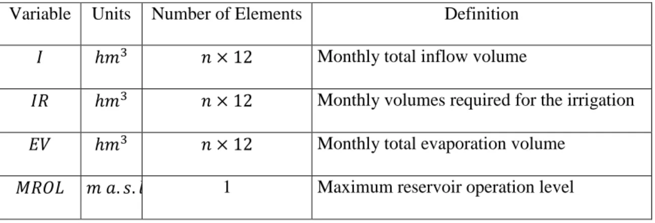
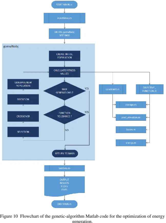
The flowchart of the Matlab code is given in Figure 10. The program “MAIN.m” controls the entire operation. It first reads the input values listed in Table 1 by calling the subprogram “inputdatas.m”. Main program initializes the vectors of lower and upper bounds for the decision variable and defines various settings for the Matlab function “gamultiobj”. Then, the “MAIN.m” calls “gamulitobj” to optimize the reservoir operation for energy generation using the method of multiobjective genetic algorithm. The names of two Matlab subprograms
“OBJECTIVE_FUNCTION.m” and “constraint.m” are sent to “gamulitobj” as arguments. Table 1 List of input variables for the Matlab genetic algorithm code. Variable Units Number of Elements Definition
𝐼 ℎ𝑚3 𝑛 × 12 Monthly total inflow volume
𝐼𝑅 ℎ𝑚3 𝑛 × 12 Monthly volumes required for the irrigation
𝐸𝑉 ℎ𝑚3 𝑛 × 12 Monthly total evaporation volume
𝑀𝑁𝑅𝑂𝐿 𝑚 𝑎. 𝑠. 𝑙 1 Minimum reservoir operation level
𝑀𝑅𝑂𝑉 ℎ𝑚3 1 Maximum reservoir operation volume
𝑀𝑁𝑅𝑂𝑉 ℎ𝑚3 1 Minimum reservoir operation volume
𝐷1 𝑚 Number of small
turbines
Penstock diameter for small turbine(s)
𝐷2 𝑚 Number of large
turbines
Penstock diameter for large turbine(s) 𝑀𝑇𝐶 ℎ𝑚3 1 Maximum monthly total storage volume that
can be allocated for energy production 𝑀𝑁𝑇𝐶 ℎ𝑚3 1 Minimum monthly total storage volume that
can be allocated for energy production 𝑇𝐶1 ℎ𝑚3 Number of small
turbines
Total volume that can be used by a small turbine operating continuously at full capacity during a month
𝑇𝐶2 ℎ𝑚3 Number of large turbines
Total volume that can be used by a large turbine operating continuously at full capacity during a month
𝑣 𝑚2/𝑠 1 Viscosity
𝐿 𝑚 Number of penstocks Penstock length
𝑘𝑠 𝑚 1 Pipe roughness
𝐼𝑅𝑉 ℎ𝑚3 1 Reservoir volume at the beginning of the simulation
The library function “gamultiobj” creates the initial population randomly by respecting the lower and upper bounds transmitted also as arguments. The fitness values 𝑃𝐸(1) and 𝑃𝐸(2) are evaluated for all chromosomes by calling the subprogram “OBJECTIVE_FUNCTION.m” and the subprogram “constraint.m”, which defines the operational constraints to operate the reservoir at a volume greater than or equal to 𝑆𝑚𝑖𝑛. To compute the objective function values, “OBJECTIVE_FUNCTION.m” calls several other subroutines:
The storage subroutine (“storage.m”) calculates the storage volume at the end of the month using (15).
Pool-elevation subroutine (“pool_elevation.m”) calculates the pool elevation corresponding to a given storage volume
The subroutine for friction losess (“losses.m”) calculates the friction loss in the penstock based on the turbine discharge. It is used only when the operation of the turbines are considered (CODE02 and CODE03).
The energy subroutine (“energy.m”) calculates the hydroelectric energy produced.
“gamultiobj” checks whether the stopping criteria is reached. If the stopping criteria is not reached, a new population is created by going through the steps of selection, crossover and mutation and a new iteration loop is executed.
If one of the stopping criteria is reached, the control is returned to the “MAIN.m”, which calls “lastdata.m” and prepares output for further analysis and plotting.
How the “OBJECTIVE_FUNCTION.m” and the various subroutines are called to accomplish specific tasks by them, requires looking into the hydraulics of hydroelectric energy generation at a dam, which is discussed in the next subsection.
Figure 10 Flowchart of the genetic-algorithm Matlab code for the optimization of energy generation.
3.4. The Concept of Energy Generation at a Dam and the Formulation of Hydropower Generation
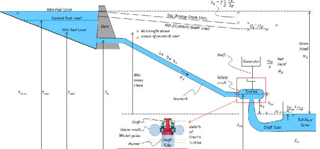
Figure 11 assumes that the hydroelectric energy is generated using a Francis turbine, which is a reaction-type turbine suitable for medium head and medium discharges [23]. The water is delivered into the spiral casing of the turbine passing through a penstock of length 𝐿𝑝 having a diameter of 𝐷𝑝 and an absolute roughness of 𝑘𝑠. The available potential energy for the production of the hydropower is equal to the gross head 𝐻𝐺, which is the vertical distance between the energy head in the pool and the energy head in the tailrace canal.
Figure 11 Hydraulics of energy generation at a dam1.
Scroll casing has openings to pass the flow into the runner, which is the rotating
component of the Francis turbine [24]. A cutaway section of the Francis turbine is shown in the insert in Figure 11. The scroll casing is designed to deliver the flow into the runner, the rotating part of the turbine, with constant velocity over its entire inner periphery. The angle of flow into
1 The figure of the Francis turbine in the insert is taken from
https://commons.wikimedia.org/wiki/File:M_vs_francis_schnitt_1_zoom.jpg. The copyright belongs to Voith-Siemens, Germany.
the runner is controlled by stay (or guide) vanes which help to transfer momentum to the blades of the runner. Runner has specially designed curved blades mounted between an upper and lower circular plate. The tangential component of the impact force of the water on the runner blade rotates the runner and the central shaft, which is connected to it. The upper end of the shaft is connected to the generator. The rate of flow through the Francis turbine is controlled by a series of wicket gates actuated by a special mechanism.
The power generated by the Francis turbine can be calculated from [22]
𝐻𝑃 = 𝜂𝜌𝑔𝑄𝐻𝑒𝑓𝑓 = 𝜂𝛾𝑄𝐻𝑒𝑓𝑓 (18)
where 𝐻𝑃 is hydroelectric power produced (Watt), 𝐻𝑒𝑓𝑓 is the net head available for turbine (m), 𝑄 is discharge from the turbine (m3/s), 𝜂 is overall turbine efficiency, 𝛾 is specific weight of water. (N/m3), 𝜌 is density of water (kg/m3), 𝑔 is gravitational acceleration (m/s2).
Although the potential energy available for the hydropower generation is given by the gross head 𝐻𝐺, due to friction losses in the penstock, the head that can be used for the energy production is the net head denoted by 𝐻𝑒𝑓𝑓. The expression for the effective head can be derived by writing the equation of conservation of energy (Bernoulli equation) between the reservoir pool and the tailrace canal as follows [23]:
𝑍𝑢 +𝑝𝑢 𝛾 + 𝑉𝑢2 2𝑔 = 𝑍𝑑 + 𝑝𝑑 𝛾 + 𝑉𝑑2 2𝑔 + ℎ𝑓+ 𝐻𝑒𝑓𝑓 (19)
The air pressure of the surface of the reservoir and the tailrace canal is atmospheric: 𝑝𝑢
𝛾 =
𝑝𝑑
𝛾 = 0
(20)
Assuming that the surface velocities at in the reservoir (upstream) and the tailrace canal (downstream) are small enough to be neglected, we write:
𝑉𝑢2
2𝑔 =
𝑉𝑑2
2𝑔 = 0
(21)
Eq. (19) can now be simplified to yield an expression for the effective head used in the energy equation, .
𝐻𝑒𝑓𝑓 = 𝑍𝑢− 𝑍𝑑 − ℎ𝑓− ℎ𝑠 = 𝐻𝐺 − ℎ𝑓− ℎ𝑠 (22) where 𝑍𝑢 is the upstream water surface elevation, 𝑍𝑑 is the downstream water surface elevation, ℎ𝑓 is the linear head loss due to friction, ℎ𝑠 is sum of all singular losses.
Note that the difference between 𝑍𝑢 and 𝑍𝑑 is the gross head 𝐻𝐺. Thus the effective head is found by subtracting linear friction losses, ℎ𝑓, and local singular losses, ℎ𝑠 (such as inlet losses, bed losses, and outlet losses) from the gross head. Usually, the penstocks are designed to minimize local losses. Therefore, in the present study, it will be assumed that the local losses are negligible; i.e. ℎ𝑠 ≅ 0.
The Darcy Weisbach equation can be used to express the friction loss in a penstock [26]
ℎ𝑓 = 𝑓𝐿𝑝 𝐷𝑝 𝑉𝑝2 2𝑔 = 𝑓 𝐿𝑝 𝐷𝑝 𝑄2 2𝑔𝐴𝑝2 (23)
where 𝑓 is the friction coefficient (Darcy Weisbach coefficient), 𝐷𝑝 is pipe diameter (m), 𝐿𝑝 is pipe length, and 𝐴𝑝 = 𝜋𝐷𝑝2/4 is the cross sectional area of the circular penstock.
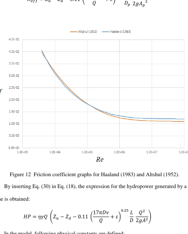
The friction coefficient 𝑓 can be calculated using Colebrook and White equation [27]. However, this is a transcendental equation that can only be solved by an iterative procedure. Several approximate explicit equations have been proposed by various researchers. These are summarized in Genić [25], who recommends the equations by Haaland (1983) and by Altshul (1952). Haaland’s equation, which is valid in the range 4 × 10³ < Re < 108 and 10−6 < ε < 5 × 10⁻², is given as
𝑓 = 1
{−1.8 ∗ 𝑙𝑜𝑔 [(3.7)𝜀 1.11+6.9𝑅𝑒 ]} 2
(24)
Altshul’s equation, which is valid in the range 4 × 10³ < Re < 108 and 10−4 < ε < 3 × 10⁻², is given as
𝑓 = 0.11 (68
𝑅𝑒+ 𝜀)
0.25 (25)
In equations of Haaland and Althsul, the relative roughness is defined as
𝜀 = 𝑘𝑠/𝐷 (26)
and the Reynolds number of the flow in the penstock is defined as, 𝑅𝑒 =𝑉𝑝𝐷𝑝 𝜈 = 𝑄𝐷𝑝 𝐴𝑝𝜈 = 𝑄𝐷𝑝 𝜋𝐷𝑝2 4 𝜈 = 4𝑄 𝜋𝐷𝑝𝜈 (27)
The equations of Haaland and Althsul plotted together in Figure 12. As it can be seen, the values of friction coefficients predicted by the two equations are quite close. For the sake of simplicity and computational efficiency, in the present thesis, it is preferred to use the equation of Altshul.
Inserting Eq. (25) in Eq (27), we get,
𝑓 = 0.11 (68𝜋𝐷𝑝𝜈 4𝑄 + 𝜀) 0.25 = 0.11 (17𝜋𝐷𝑝𝜈 𝑄 + 𝜀) 0.25 (28)
By inserting Eq. (28) in Eq. (23), one obtains the expression for the friction head loss
ℎ𝑓 = 0.11 (17𝜋𝐷𝑝𝜈 𝑄 + 𝜀) 0.25𝐿 𝑝 𝐷𝑝 𝑄2 2𝑔𝐴𝑝2 (29)
The subprogram “losses.m” uses Eq. (29) to calculate the head loss due to friction. The expression for the effective head is then obtained by inserting Eq. (29) in Eq. (22):
𝐻𝑒𝑓𝑓 = 𝑍𝑢− 𝑍𝑑 − 0.11 (17𝜋𝐷𝑝𝜈 𝑄 + 𝜀) 0.25𝐿 𝑝 𝐷𝑝 𝑄2 2𝑔𝐴𝑝2 (30)
Figure 12 Friction coefficient graphs for Haaland (1983) and Altshul (1952). By inserting Eq. (30) in Eq. (18), the expression for the hydropower generated by a turbine is obtained: 𝐻𝑃 = 𝜂𝛾𝑄 (𝑍𝑢− 𝑍𝑑− 0.11 (17𝜋𝐷𝜈 𝑄 + 𝜀) 0.25𝐿 𝐷 𝑄2 2𝑔𝐴2) (31)
In the model, following physical constants are defined:
The total turbine efficiency is accepted to be approximately 0.918. It is assumed that there is constant efficiency in the turbines for each flow rate.
Viscosity of water is taken as 1.00 × 10⁻⁶𝑚2/s. Gravitational acceleration is taken as 9.81 𝑚/𝑠2.
The tailrace elevation 𝑍𝑑 requires computation of the discharge rating curve for the cross section at the downstream of the dam. In the present thesis, however, it is assumed that the variation of the water surface elevation with the discharge is negligible, and the user will provide a constant value as input data.
3.5. Final Considerations for the Matlab Code with Genetic Algorithm
In Section 3.2, it was shown that the computation of end of the month storage volume computed using Eq. (15). The hydropower generation is computed using the pool elevation corresponding end of the month storage volume. In order to do that, the program needs the relationship between the reservoir pool elevation and the storage volume, which is normally available for a given reservoir as stage-volume curve. This point will be discussed later in more detail when presenting the test case data. In the Matlab code, subprogram “storage.m” calculates the end of the month storage volume using Eq. (15). This value is then used by the subprogram “pool_elevation.m” to calculate and return the corresponding pool elevation.
The genetic algorithm code requires at least one stopping criteria to stop the generation of new population and terminate the program. Since this is a multiobjective optimization, there can be more than one optimum solution. The fitness values of the population must be analyzed to select the best solutions.
In the program, this is achieved by the subprogram “lastdata.m”, which is called by the “MAIN.m” when the genetic algorithm encounters the stopping criteria. The selection of the best chromosome is achieved using a weighted sum of the index values for the two objective
functions and the total amount of storage volume released from the reservoir. The subprogram “lastdata.m” performs the following operations:
For each chromosome in the population, the sum of the total energy produced over the 𝑚-year study period, 𝑇𝑃𝐸, is calculated. Based on this total, an integer index value, 𝐼𝑇𝐸, is assigned to the chromosome. The integer index value corresponds to the quotient obtained by dividing the 𝑇𝑃𝐸 by a suitable interval value, for example 100 GWh in the present case.
For each chromosome in the population, the sum of the total firm produced over the 𝑚-year study period, 𝑇𝐹𝐸, is calculated. Based on this total, an integer index value, 𝐼𝐹𝐸, is assigned to the chromosome. The integer index value corresponds to the quotient obtained by dividing the 𝑇𝐹𝐸 by a suitable interval value, for
example 5 GWh in the present case.
For each chromosome in the population, the total overflow volume released to downstream over the 𝑚-year study period, 𝑉𝑂𝐹, is calculated. Based on this total, an integer index value, 𝐼𝑂𝐹, is assigned to the chromosome. The integer index value corresponds to the quotient obtained by dividing the 𝑉𝑂𝐹 by a suitable interval value, for example 5 hm3 in the present case.
The best chromosome is then calculate using the following formula:
𝐵𝑒𝑠𝑡 𝐶ℎ𝑟𝑜𝑚𝑜𝑠𝑜𝑚𝑒 = 𝑇𝑃𝐸 × 𝑤𝑇𝑃𝐸 + 𝑇𝐹𝐸 × 𝑤𝑇𝐹𝐸+ 𝑉𝑂𝐹 × 𝑤𝑉𝑂𝐹 (32)
where 𝑤𝑇𝑃𝐸 = 0.50, 𝑤𝑇𝐹𝐸 = 0.25, and 𝑤𝑉𝑂𝐹 = 0.25 are the weighting coefficients. Since, the present study focuses on the energy production; the weighting coefficient 𝑤𝑇𝑃𝐸 is chosen to be greater than the other two. The weight coefficient values are highly subjective and problem dependent. They can be defined according to the order