Abstract—The main purpose of robot calibration is the correction of the possible errors in the robot parameters. This paper presents a method for a kinematic calibration of a parallel robot that is equipped with one camera in hand. In order to preserve the mechanical configuration of the robot, the camera is utilized to acquire incremental positions of the end effector from a spherical object that is fixed in the word reference frame. Incremental positions of the end effector are related to incremental positions of encoders of the motors of the robot. A kinematic model of the robot is modified in order to take into account possible errors of kinematic parameters. The solution of the model utilizes incremental positions of the resolvers and end effector, the new parameters minimizes errors in the kinematic equations. Spherical properties and intrinsic camera parameters are utilized to model sphere projection in order to improve spatial measurements. The robot system is designed to carry out tracking tasks and the calibration of the system is finally validated by means of integrating the errors of the visual controller.
I. INTRODUCTION
CCURACY is a crucially important performance
specification for parallel kinematic machines (PKM), particularly for those that are involved in tasks as can be surgery, material machining, electronics manufactory, products assembling, among other. In this work calibration method is used to improve a widely studied image based visual controller [1]. In contrast to serial robots, parallel robots (or parallel kinematic machines) are characterized by high structural stiffness, high load operation, high speed and acceleration of the end effector and, high accuracy for end effector positioning. This accuracy, however, relies on a robust and accurate calibration, which is a difficult problem both from a theoretical and a practical point of view, even if it may be performed off-line. Robot accuracy can be affected by increasing backlash due to robot operation, thermal effects, elements deformation [2], robot control and manufacturing errors. Although hybrid calibration methods exist, in general, it is possible to classify different calibration
Manuscript received March 8, 2010. This work was supported in part by the Universidad Politécnica de Madrid and International Cooperation Spanish Agency (AECI), A/026481/09.
A. Traslosheros and J. M. Sebastián are with the Technical University of Madrid, DISAM, José Gutierrez Abascal 2, CO 28003 Spain. Phone (+34) 913 363 061, email: [email protected] and [email protected]. E. Castillo is with the National Technical Institute of Mexico, Departament of Mechatronics, Cerro Blanco No. 141., CO 76090, Queretaro, Mexico. Phone (+52) 442 229 0804, email: [email protected]
F. Roberti and R. Carelli are with the National University of San Juan, Av. San Martín Oeste 1109, CO 5400 Argentina. Phone (+54) 0264 4 213 303, email: [email protected] and [email protected]. Department of Automatics, National University of San Juan, Argentina.
strategies in three main groups (by considering the location of measurement instruments and its additional elements): External calibration, it is based on measurements of the positions of the end effector (or other structural element) of the robot by means of an external instrument. Constrained calibration groups those methods that rely on mechanical elements in order to constraint some kind of motion of the robot during the calibration process, this method is generally simple and it is considered the most inexpensive. And finally, auto calibration that consist on that methods that calibrates the robot automatically and even during the robot operation [3], in general auto (or self) calibration method is more expensive due to its complexity and even it includes redundant sensors [4] or elements. External calibration can be done by measuring completely or partially the pose parameters of the platform. Measurements of the pose of a platform can be done with a laser and a coordinate measuring machine (CMM)[5], commercial visual systems (optical system and infrared light) [6], laser sensor [7], by adding passive legs [8], with a interferometer [9], by a LVDT and inclinometers in [10] [11], theodolite [12], with gauges [13], with double ball bar (DBB) [14], by inspecting a machined part that is dedicated to the calibration process [15], accelerometers [16], or with visual systems and patterns widely studied (chess-board) [17][18][19]. Above examples are different strategies that obtain kinematic information of the robot but in general, calibration methods impose virtual or real constraints on the poses of the end effector (or mobile elements). By choosing the appropriate method, a calibration can be an economical and practical technique for improve accuracy of a PKM [20].
The principle of the calibration process is to get the constraints at a large enough number of measured poses (called calibration poses) in order to conclude which is the best geometry (distances or angles of elements) of the robot that satisfies them. The basic idea it has been applied to calibration of serial and parallel robots and the main difference has been the measurement instruments and strategies. Visual methods are becoming more popular due to its simplicity and because it can be an inexpensive method in comparison to others, for parallel robots it was first proposed by Amirat [21]. Visual methods that propose a monocular system [17][18][19] propose to utilize a pattern (marks on a flat surface), these kind of patterns are employed in camera calibration where it is possible to obtain intrinsic and extrinsic parameters [22]. By means of the extrinsic parameters of the camera it is possible (by attaching the camera or the pattern to the rend effector of the robot) to obtain the pose of the end effector of the robot and
One Camera in Hand for Kinematic Calibration of a Parallel Robot
Alberto Traslosheros, José María Sebastián, Eduardo Castillo, Flavio Roberti, Ricardo CarelliA
consequently those poses can be considered as calibration poses.
In this paper an economical and external calibration method is proposed to calibrate a parallel robot of 3 DOF. The proposed method utilizes positions from the resolvers of the motors and visual information that is obtained from a spherical element (in order to obtain joints and 3D incremental positions). Once the above information is obtained then it is replaced in the constraint equations in order to solve numerically and obtain the best set of geometrical parameters that satisfies the set of equations. Finally calibrated parameters are used in an image visual servoing controller and compared to the controller that utilizes nominal parameters.
II. SYSTEM DESCRIPTION
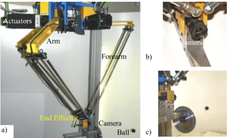
The main objective of proposed method it is to calibrate the parallel robot of the system called: Robotenis. Calibration of the robot is required in order to improve its accuracy in visual servoing algorithms and develop future tasks as can be the Ping-Pong game. Robotenis was designed in order to study and design visual servoing controllers and to carry out object tracking under dynamic environments. The mechanical structure of system Robotenis is inspired by the DELTA robot [23][24] and its vision system is based in one camera allocated at the end effector of the robot. Basically, the platform Robotenis (Fig. 1 a) consists of a parallel robot and a visual system for acquisition and analysis. The maximum end effector speed of the parallel robot is 6𝑚𝑚 𝑠𝑠⁄ and its maximum acceleration is 58𝑚𝑚 𝑠𝑠⁄ 2. The visual system of the platform Robotenis [25] is composed of a 50 grams camera that is located at the end effector (Fig. 1 b) and a frame grabber (SONY XCHR50 and Matrox Meteor 2-MC/4 respectively). The motion system is composed of three AC brushless servomotors, Ac drivers (Unidrive), planetary gearboxes and the joint controller is implemented in a DS1103 card (implemented in ANSI C).
Fig. 1 a) System Robotenis, b) Robot camera, c) Robot environment III. CONSTRAINTEQUATIONS
Constraint equations of the calibration method were obtained from a kinematic model of the robot. It is important
to bring out that in the constraint equations, transformation matrix from the camera to the end effector is not considered.
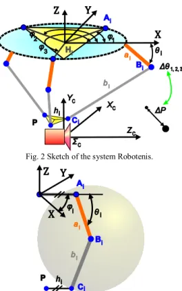
Transformation matrix was divided in its rotation and translation, rotation matrix was obtained independently to the robot calibration, on the other hand translation matrix is not necessary, because the camera is fixed to the end effector and the model of the constraint equations is an incremental one. In the Fig. 2 it is shown a sketch of the parallel robot, where 𝑶𝑶𝒙𝒙𝒙𝒙𝒙𝒙 is the robot reference frame, 𝑎𝑎𝑖𝑖 are arm lengths, 𝑏𝑏𝑖𝑖 are forearm lengths, arms and forearms are connected in 𝑩𝑩𝒊𝒊 , 𝐻𝐻𝑖𝑖 are distances from the robot reference frame (𝑶𝑶𝒙𝒙𝒙𝒙𝒙𝒙) to the revolute axis of motors (𝑨𝑨𝒊𝒊 ), ℎ𝑖𝑖 are the distances from the center of the end effector (𝑷𝑷) to the forearm (𝑪𝑪𝒊𝒊), 𝜃𝜃𝑖𝑖 are the motor angles from a home position (unknown), 𝜙𝜙𝑖𝑖 is the angle in which point 𝑨𝑨𝒊𝒊 is allocated in the plane 𝑋𝑋𝑋𝑋 of the robot frame reference and 𝑖𝑖 = 1,2,3.
Constraint equations are based on the movement of the forearms respect to the robot arms. [26]. In the Delta robot, forearms are parallelograms that link the end effector to the arms by means of spherical joints. Spherical joints allow modeling the movement of the end effector as the intersection of three spherical surfaces that are described by points 𝑪𝑪𝒊𝒊 in Fig. 3. By inspecting Fig. 2 and Fig. 3 it is possible to obtain the surface of a sphere described by the point 𝑪𝑪𝒊𝒊 with center in 𝑩𝑩𝒊𝒊 as:
Γ𝑖𝑖= (𝐶𝐶𝑖𝑖𝑖𝑖− 𝐵𝐵𝑖𝑖𝑖𝑖)2+�𝐶𝐶𝑖𝑖𝑖𝑖− 𝐵𝐵𝑖𝑖𝑖𝑖�2+ (𝐶𝐶𝑖𝑖𝑖𝑖− 𝐵𝐵𝑖𝑖𝑖𝑖)2− 𝑏𝑏𝑖𝑖2= 0 (1) Where 𝑩𝑩𝒊𝒊 and 𝑪𝑪𝒊𝒊 can be expressed in the robot frame as:
�𝐵𝐵𝐵𝐵𝑖𝑖𝑖𝑖 𝐵𝐵𝑖𝑖 � 0𝑖𝑖𝑖𝑖𝑖𝑖 𝑖𝑖 =�((𝐻𝐻𝐻𝐻++𝑎𝑎𝑎𝑎𝑐𝑐𝜃𝜃𝑐𝑐𝜃𝜃) ) 𝑐𝑐𝜙𝜙𝑠𝑠𝜙𝜙 𝑎𝑎𝑠𝑠𝜃𝜃 �𝑖𝑖 �𝐶𝐶𝐶𝐶𝑖𝑖𝑖𝑖 𝐶𝐶𝑖𝑖 � 0𝑖𝑖𝑖𝑖𝑖𝑖 𝑖𝑖 =�𝑃𝑃𝑃𝑃𝑖𝑖𝑖𝑖 𝑃𝑃𝑖𝑖 � − �𝑐𝑐𝜙𝜙 −𝑠𝑠𝜙𝜙𝑠𝑠𝜙𝜙 𝑐𝑐𝜙𝜙 00 0 0 1�𝑖𝑖 �−ℎ0 0 �𝑖𝑖 (2)
Note that in above equations 𝑐𝑐𝜃𝜃𝑖𝑖 = cos𝜃𝜃𝑖𝑖, 𝑠𝑠𝜃𝜃𝑖𝑖 = sin𝜃𝜃𝑖𝑖, 𝑷𝑷 =�𝑃𝑃𝑖𝑖 ,𝑃𝑃𝑖𝑖,𝑃𝑃𝑖𝑖�′, 𝑩𝑩𝒊𝒊=�𝐵𝐵𝑖𝑖 ,𝐵𝐵𝑖𝑖,𝐵𝐵𝑖𝑖�𝑖𝑖′, etc. By other hand by supposing that we can obtain incremental joint and end effector positions we have that each absolute measurement can be expressed as:
𝜃𝜃𝑖𝑖𝑖𝑖=𝜃𝜃𝑖𝑖0+Θ𝑖𝑖𝑖𝑖 and 𝑷𝑷𝑖𝑖 =𝑷𝑷0+𝚷𝚷𝑖𝑖 (3) Observe that 𝜃𝜃𝑖𝑖0 and 𝑷𝑷𝟎𝟎 are unknown and, 𝛩𝛩𝑖𝑖𝑖𝑖 = 𝛥𝛥𝜃𝜃𝑖𝑖𝑖𝑖 = 𝜃𝜃𝑖𝑖𝑖𝑖 – 𝜃𝜃𝑖𝑖(𝑖𝑖−1) and 𝚷𝚷k= 𝛥𝛥𝑷𝑷𝑖𝑖= 𝑷𝑷𝑖𝑖− 𝑷𝑷𝑖𝑖−1 are incremental
measuring (obtained from resolvers and camera): 𝐕𝐕k =�𝛩𝛩1,𝛩𝛩2,𝛩𝛩3,𝛱𝛱𝑖𝑖 ,𝛱𝛱𝑖𝑖,𝛱𝛱𝑖𝑖�𝑖𝑖, where 𝚷𝚷𝐤𝐤 are measured and are parameters that are expressed as incremental positions of the end effector and they are measured from sphere images (section V), 𝑖𝑖 is the incremental measurement number.
IV. SOLUTION OF THE CONSTRAINTS EQUATIONS
Not all parameters of the robot have effect on the kinematic model and as a consequence they cannot be identified, this is known as observability. An observability measure can be derived from the Jacobian of the constraint equations. This
Ball
Actuators
Arm
Forearm
End Effector Camera
Camera
c) b)
Jacobian is called the observation matrix and observable parameters can be obtained by its 𝐐𝐐𝐐𝐐 decomposition [27]. In our model by means of the 𝐐𝐐𝐐𝐐 decomposition influence of the parameters 𝜙𝜙𝑖𝑖 and 𝐻𝐻𝑖𝑖 are difficult to observe in the model, for this reason they are not identified in this work and them nominal value is taken into account. On the other hand identifiable parameters are: 𝑎𝑎𝑖𝑖 , 𝑏𝑏𝑖𝑖, ℎ𝑖𝑖 and reference position of the actuators and the end effector of the robot: 𝜃𝜃𝑖𝑖0 and 𝑷𝑷𝟎𝟎 respectively (𝑖𝑖 = 1, 2, 3 and 𝑷𝑷𝟎𝟎 is the initial end effector position). Thus unknown parameters can be expressed as:
𝒖𝒖𝒊𝒊 = [𝑎𝑎𝑖𝑖 ,𝑏𝑏𝑖𝑖 ,ℎ𝑖𝑖 ,𝜃𝜃𝑖𝑖0] and 𝑼𝑼 = [𝑢𝑢1 𝑢𝑢2 𝑢𝑢3 𝑃𝑃𝑖𝑖0 𝑃𝑃𝑖𝑖0 𝑃𝑃𝑖𝑖0]
And substituting incremental equations (3) in (2) and (1), constraint equations can be arranged as:
Γi =�(𝑎𝑎𝑖𝑖𝑐𝑐(𝜃𝜃𝑖𝑖 + 𝛩𝛩𝑖𝑖𝑖𝑖 ) +𝐻𝐻𝑖𝑖 ) 𝑐𝑐𝜙𝜙𝑖𝑖 – 𝑃𝑃𝑖𝑖 − ℎ𝑖𝑖𝑐𝑐𝜙𝜙𝑖𝑖 – Π𝑖𝑖𝑖𝑖�2 +�(𝑎𝑎𝑖𝑖𝑐𝑐(𝜃𝜃𝑖𝑖 + 𝛩𝛩𝑖𝑖𝑖𝑖 ) +𝐻𝐻𝑖𝑖 ) 𝑠𝑠𝜙𝜙𝑖𝑖 – 𝑃𝑃𝑖𝑖 − ℎ𝑖𝑖𝑠𝑠𝜙𝜙𝑖𝑖 – Π𝑖𝑖𝑖𝑖�
2 +(𝑎𝑎𝑖𝑖𝑠𝑠(𝜃𝜃𝑖𝑖 + 𝛩𝛩𝑖𝑖𝑖𝑖 )– 𝑃𝑃𝑖𝑖 – Π𝑖𝑖𝑖𝑖)2− 𝑏𝑏𝑖𝑖2= 0
(4)
In order to solve, equations in (4) are grouped as:
Φ(U, V𝑖𝑖) = [Γ11, … ,Γ1𝑖𝑖,Γ21, … ,Γ2𝑖𝑖,Γ31, … ,Γ3𝑖𝑖]′ (5) Note that constraint equations are not linear, its solution is no exactly satisfied thus commonly a nearly solution is obtained by numerical algorithms as can be Gauss-Newton. Expressing constraints (5) in them Taylor linear approximation in order to solve iteratively.
Φ(𝑈𝑈𝑛𝑛+1 ,𝑉𝑉𝑖𝑖)≈ Φ(𝑈𝑈𝑛𝑛,𝑉𝑉𝑖𝑖) +𝐽𝐽(𝑈𝑈𝑛𝑛,𝑉𝑉𝑖𝑖) (𝑈𝑈𝑛𝑛+1− 𝑈𝑈𝑛𝑛 ) = 0 (6) Where 𝑛𝑛 is the iteration number and 𝐽𝐽3𝑖𝑖×18 is the Jacobian
of the constraint equations or the observation matrix that it is given by: 𝐽𝐽(𝑈𝑈𝑛𝑛,𝑉𝑉𝑖𝑖) =� 𝐽𝐽1𝑖𝑖 𝐽𝐽2𝑖𝑖 𝐽𝐽3𝑖𝑖 � 𝐽𝐽1𝑖𝑖= ⎣ ⎢ ⎢ ⎢ ⎢ ⎡∂Γ11 ∂𝑎𝑎1… ∂Γ11 ∂𝜃𝜃10, 0, … ,0,0, … ,0, ∂Γ11 ∂𝑃𝑃𝑖𝑖0, ∂Γ11 ∂𝑃𝑃𝑖𝑖0, ∂Γ11 ∂𝑃𝑃𝑖𝑖0 ⋮ ∂Γ1𝑖𝑖 ∂𝑎𝑎1… ∂Γ1𝑖𝑖 ∂𝜃𝜃10, 0, … ,0,0, … ,0, ∂Γ1𝑖𝑖 ∂𝑃𝑃𝑖𝑖0, ∂Γ1𝑖𝑖 ∂𝑃𝑃𝑖𝑖0, ∂Γ1𝑖𝑖 ∂𝑃𝑃𝑖𝑖0⎦⎥ ⎥ ⎥ ⎥ ⎤ 𝐽𝐽2𝑖𝑖= ⎣ ⎢ ⎢ ⎢ ⎢ ⎡0, … ,0,∂Γ∂𝑎𝑎21 2 … ∂Γ21 ∂𝜃𝜃20, 0, … ,0, ∂Γ21 ∂𝑃𝑃𝑖𝑖0, ∂Γ21 ∂𝑃𝑃𝑖𝑖0, ∂Γ21 ∂𝑃𝑃𝑖𝑖0 ⋮ 0, … ,0,∂Γ∂𝑎𝑎2𝑖𝑖 2 … ∂Γ2𝑖𝑖 ∂𝜃𝜃20, 0, … ,0, ∂Γ2𝑖𝑖 ∂𝑃𝑃𝑖𝑖0, ∂Γ2𝑖𝑖 ∂𝑃𝑃𝑖𝑖0, ∂Γ2𝑖𝑖 ∂𝑃𝑃𝑖𝑖0⎦⎥ ⎥ ⎥ ⎥ ⎤ 𝐽𝐽3𝑖𝑖= ⎣ ⎢ ⎢ ⎢ ⎢ ⎡0, … ,0,0, … ,0,∂Γ∂𝑎𝑎31 3 … ∂Γ31 ∂𝜃𝜃30, ∂Γ31 ∂𝑃𝑃𝑖𝑖0, ∂Γ31 ∂𝑃𝑃𝑖𝑖0, ∂Γ31 ∂𝑃𝑃𝑖𝑖0 ⋮ 0, … ,0,0, … ,0,∂Γ∂𝑎𝑎3𝑖𝑖 3 … ∂Γ3𝑖𝑖 ∂𝜃𝜃30, ∂Γ3𝑖𝑖 ∂𝑃𝑃𝑖𝑖0, ∂Γ3𝑖𝑖 ∂𝑃𝑃𝑖𝑖0, ∂Γ3𝑖𝑖 ∂𝑃𝑃𝑖𝑖0⎦⎥ ⎥ ⎥ ⎥ ⎤ (7)
Finally parameters are iteratively obtained by:
Un+1 = Un − J(Un, Vk)+Φ(Un,Vk) (8)
Where 𝐽𝐽+ is the Jacobian pseudoinverse. Initial values (𝑈𝑈0) are given by the nominal parameters and a pose of the robot (given from nominal parameters). In the constraint equations in (4), units of the Jacobian (7) are homogeneous and Jacobian is not necessary to normalize
Fig. 2 Sketch of the system Robotenis.
Fig. 3 One leg profile of the system Robotenis. V. VISUAL MEASUREMENT SYSTEM Visual measurement system is composed by a fixed ball (hanging by a thread) and a calibrated camera that it is allocated on the end effector of the robot. Initial positions of resolvers are registered; incremental positions are measured by the visual system and both measures related by constraint equations to solve unknown parameters.
A. Selection of Calibration Poses
In order to solve the constraint equations system a set of incremental (resolvers and end effector) poses is needed, simulations shows that 6 different poses are at least required (perfect measurements). However perfect measurements do not exist and is necessary to choose best calibration poses. Thus, errors in the parameters of the robot are especially critical when the calibration pose is near from a singularity. However in a practical calibration process, if poses are extremely near of singularities, those poses are able to produce unpredictable movements (due to kinematic errors). In this work, the robot workspace is numerically well known (by using nominal values) and the calibration poses are chosen randomly from the workspace boundaries. Thus if a pose is between 5 and 10 cm away from a singularity, then the pose is included as a calibration pose. Experiments were implemented with 300 of poses and each measure is the mean of 500 images in order to avoid noise from image acquisition (image acquisition rate: 8.34 𝑚𝑚𝑠𝑠). Due to its simplicity, calibration process is done automatically in 21 minutes and it is possible to calibrate on-line.
On the other hand, a spherical object has been chosen as reference of the end effector and some considerations of the
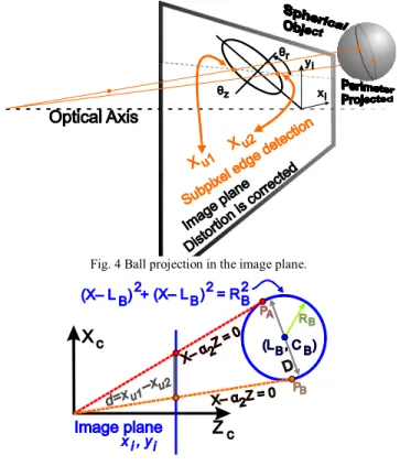
spherical object and its projection on the image plane has to be taken into account, Fig. 4. Each measurement is done in two iterative steps, first a simplified model is considered as in Fig. 5 where two sub-pixel points are acquired from the image (distortion is previously corrected), secondly a correction of measurements is done by considering elliptical projection of the ball.
B. Simplified Ball Projection Model
Objective of this method is to obtain the position of the center of a spherical object. Position is obtained from the projection of the ball in the plane of the image. The method takes into account that the projected ball does not correspond to the real center and diameter of the ball. Proposed method is iterative and a first approximation is obtained by a simplified 2D model as shown in fig. 5. Model in fig. 5 is contained in a plane in the coordinates 𝑋𝑋 and 𝑍𝑍 that are in the camera coordinate frame (𝑋𝑋𝑐𝑐 ,𝑋𝑋𝑐𝑐 ,𝑍𝑍𝑐𝑐 ). On the other hand points that are in the image are related by a line that is tangent to the sphere and passes through optical center of the camera, that is:
𝑋𝑋=𝛼𝛼1𝑍𝑍 and 𝑋𝑋=𝛼𝛼2𝑍𝑍 (9)
Sphere is fixed in the space, its diameter is known (38mm) and the distance of the line that is tangent to the perimeter to the center of the sphere (𝐿𝐿𝐵𝐵,𝐶𝐶𝐵𝐵) are related by: 𝑅𝑅𝐵𝐵 = 𝐿𝐿𝐵𝐵 – 𝛼𝛼𝐶𝐶𝐵𝐵
√1 + 𝛼𝛼2 (10)
Where 𝑅𝑅𝐵𝐵 = 19𝑚𝑚𝑚𝑚 and 𝛼𝛼 can be cleared from eq.(10): 𝛼𝛼1,2 = 𝐿𝐿𝐵𝐵𝐶𝐶𝐵𝐵±�𝐿𝐿𝐵𝐵
2𝐶𝐶
𝐵𝐵2 −(𝐶𝐶𝐵𝐵2 – 𝑅𝑅𝐵𝐵2 )(𝐿𝐿2𝐵𝐵 – 𝑅𝑅𝐵𝐵2) 𝐶𝐶𝐵𝐵2 – 𝑅𝑅𝐵𝐵2
(11)
Where 𝐶𝐶𝐵𝐵 is supposed positive and 𝐶𝐶𝐵𝐵>𝑅𝑅𝐵𝐵 , otherwise the ball cannot be seen. By substituting eq. (10) and (9) in the following circumference equation from Fig. 5:
�𝛼𝛼1,2𝑍𝑍 – 𝐿𝐿𝐵𝐵�2 + (𝑍𝑍 – 𝐶𝐶𝐵𝐵)2 = 𝑅𝑅𝐵𝐵2 (12) Clearing for 𝑍𝑍 and simplifying it is possible to obtain: 𝑍𝑍1,2=𝛼𝛼1,2𝛼𝛼𝐿𝐿𝐵𝐵 + 𝐶𝐶𝐵𝐵
1,22 + 1 (13)
Thus the purpose is to obtain the center of the ball (𝐿𝐿𝐵𝐵,𝐶𝐶𝐵𝐵) from the known points in the image (𝑖𝑖𝑢𝑢1,𝑖𝑖𝑢𝑢2). For points that are tangent to the sphere it is easy to see that: 𝑋𝑋1 𝑍𝑍1= 𝑖𝑖𝑢𝑢1 𝑓𝑓 ; 𝑋𝑋2 𝑍𝑍2= 𝑖𝑖𝑢𝑢2 𝑓𝑓 (14)
Where 𝑓𝑓 is the focal distance. The algorithm that is implemented is iterative and its solution is obtained in a few iterations. Initial solution is obtained supposing that:
𝑍𝑍1≈ 𝑍𝑍2≈ 𝐶𝐶𝑏𝑏 ; �𝑋𝑋2– 𝑋𝑋1�= 2𝑅𝑅𝐵𝐵 (15) In equation (11) parameters 𝐿𝐿𝐵𝐵 and 𝐶𝐶𝐵𝐵 are the position of the center (𝑋𝑋𝐵𝐵 = 𝐿𝐿𝐵𝐵 and 𝑍𝑍𝐵𝐵= 𝐶𝐶𝐵𝐵) of the circle in Fig. 5 and they are unknown. At this point, must be cleared that the algorithm is iterative and it needs an initial position that is given by:
𝐶𝐶𝐵𝐵 =|𝑖𝑖𝑢𝑢22𝑓𝑓𝑅𝑅−𝑖𝑖𝐵𝐵𝑢𝑢1| and 𝐿𝐿𝐵𝐵=𝑖𝑖𝑢𝑢22+𝑓𝑓𝑖𝑖𝑢𝑢1 𝐶𝐶𝐵𝐵 (16) Values obtained in eq. (16) and equations (11), (13) and (14) are iteratively utilized to obtain 𝐶𝐶𝐵𝐵 and 𝐿𝐿𝐵𝐵 that are repeatedly substituted in eq. (12) until there are not differences between old and new values.
Fig. 4 Ball projection in the image plane.
Fig. 5 Ball projection in the image plane.
A. Ellipse Ball Projection in 𝑍𝑍 correction
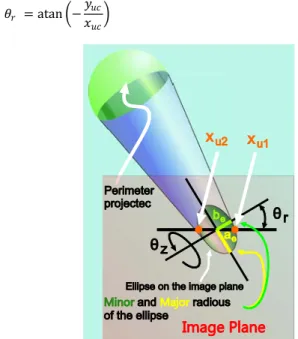
One condition of the method is that the spherical object must be fully visible. This condition guarantees that the projection of the sphere is an ellipse Fig. 6 (or a circumference if the projection lies on the center of the image). Note in Fig. 6 that 𝑖𝑖𝑢𝑢1 and 𝑖𝑖𝑢𝑢2 are not on the axis of the projected ellipse, thus the diameter considered in the calculus of Z contains a small error due to the projected ball.
In order to correct the diameter that is considered in the calculus of Z, the minor axis of the ellipse has to be calculated. Once the minor axis is calculated then 2𝑏𝑏𝑒𝑒 is replaced in (16) instead of |𝑖𝑖𝑢𝑢2 – 𝑖𝑖𝑢𝑢1|, thus the ball position is calculated by earlier method for a second time. This second step mainly depends on angle 𝜃𝜃𝑖𝑖 and the method stops when 𝜃𝜃𝑖𝑖 is constant or almost constant (usually two or three cycles). 𝜃𝜃𝑖𝑖 is the angle between the optical axis and the line that passes through the center of the ball and the center of the projected ball. Note that 𝜃𝜃𝑖𝑖 coincides with the angle that the image plane can be rotated around the minor axis of the ellipse in order to project a circle on the plane image, thus:
𝜃𝜃𝑖𝑖= acos� 𝑍𝑍
�(𝑋𝑋2+𝑋𝑋2+𝑍𝑍2� (17)
θr θr θr θr , yuc xuc xu1 xue= xu1 xue= xu1 xue= xu1 xue= Centroid
ellipse are related by:
𝑏𝑏𝑒𝑒= 𝑎𝑎𝑒𝑒 cos(𝜃𝜃𝑖𝑖) (18)
The projected ellipse in its rotated canonical parametric form can be expressed as:
𝑖𝑖𝑢𝑢𝑒𝑒=𝑏𝑏𝑒𝑒cos(𝜃𝜃𝑒𝑒) cos(𝜃𝜃𝑟𝑟) –𝑎𝑎𝑒𝑒sin(𝜃𝜃𝑒𝑒) sin(𝜃𝜃𝑟𝑟) +𝑖𝑖𝑢𝑢𝑐𝑐 𝑖𝑖𝑢𝑢𝑒𝑒 = 𝑏𝑏𝑒𝑒cos(𝜃𝜃𝑒𝑒) sin(𝜃𝜃𝑟𝑟 ) +𝑎𝑎𝑒𝑒sin(𝜃𝜃𝑒𝑒) cos(𝜃𝜃𝑟𝑟 ) +𝑖𝑖𝑢𝑢𝑐𝑐
(19)
Where 𝜃𝜃𝑒𝑒 is the angle of a point in the canonical form of the ellipse, 𝜃𝜃𝑟𝑟 is the angle that the ellipse is rotated around the 𝑍𝑍 axis of the camera (eq. (20)) and (𝑖𝑖𝑢𝑢𝑐𝑐,𝑖𝑖𝑢𝑢𝑐𝑐) is the center of the ellipse in the image, Fig. 7.
𝜃𝜃𝑟𝑟 = atan�−𝑖𝑖𝑖𝑖𝑢𝑢𝑐𝑐
𝑢𝑢𝑐𝑐� (20)
Fig. 6 Ellipse of the sphere projection on the image plane.
Fig. 7 Angle 𝜃𝜃𝑟𝑟.
On the other hand we know that (𝑖𝑖𝑢𝑢1,𝑖𝑖𝑢𝑢1 ) and (𝑖𝑖𝑢𝑢2,𝑖𝑖𝑢𝑢2) belong to the ellipse, and by simple inspection in Fig. 6: 𝑖𝑖𝑢𝑢𝑐𝑐− 𝑖𝑖𝑢𝑢𝑒𝑒 = (𝑖𝑖𝑢𝑢2− 𝑖𝑖𝑢𝑢1)⁄2 , 𝑖𝑖𝑢𝑢𝑐𝑐 − 𝑖𝑖𝑢𝑢𝑒𝑒 = (𝑖𝑖𝑢𝑢2− 𝑖𝑖𝑢𝑢1)⁄ 2 = 0 and substituting in (19) we can obtain that:
(𝑖𝑖𝑢𝑢2− 𝑖𝑖𝑢𝑢1) 2⁄ =𝑏𝑏𝑒𝑒cos(𝜃𝜃𝑒𝑒) cos(𝜃𝜃𝑟𝑟 ) –𝑎𝑎𝑒𝑒sin(𝜃𝜃𝑒𝑒) sin(𝜃𝜃𝑟𝑟) 0 =𝑏𝑏𝑒𝑒cos(𝜃𝜃𝑒𝑒) sin(𝜃𝜃𝑟𝑟) + 𝑎𝑎𝑒𝑒sin(𝜃𝜃𝑒𝑒) cos(𝜃𝜃𝑟𝑟) (21) Substituting (18) in (21) and clearing for 𝑎𝑎𝑒𝑒 and 𝜃𝜃𝑒𝑒 finally: 𝑎𝑎𝑒𝑒=�cos(𝜃𝜃 (𝑖𝑖𝑢𝑢2− 𝑖𝑖𝑢𝑢1) 2⁄
𝑖𝑖) cos(𝜃𝜃𝑒𝑒) cos(𝜃𝜃𝑟𝑟 ) – sin(𝜃𝜃𝑒𝑒) sin(𝜃𝜃𝑟𝑟)� 𝜃𝜃𝑒𝑒 = atan(−tan(𝜃𝜃𝑟𝑟 ) cos (𝜃𝜃𝑖𝑖))
(22)
VI. RESULTS
In order to test the calibration method, nominal parameters and calibrated parameters are compared when they are utilized in an image based visual controller. The robot and its visual controller are designed with the purpose of carry out tracking tasks, for more information please consults [28]. Visual controller is based in a well established architecture called: dynamic image-based look-and-move visual servoing. In this scheme visual controller makes use of image estimates (position, velocity), Jacobian of the robot and its kinematic model in order to act over the robot actuators. Thus errors in the kinematic model generate undesirable movements that have an effect on the performance of the visual controller. In this section we compare the performance of the visual controller of the robot when the controller makes use of the nominal kinematic parameters and calibrated kinematic parameters (shown in table 1). In order to compare the visual controller, a tracking index performance (𝑇𝑇𝑇𝑇𝑃𝑃) is defined as follows:
𝑇𝑇𝑇𝑇𝑃𝑃=∑∑𝑁𝑁𝑖𝑖=1|𝑒𝑒(𝑖𝑖)|
� 𝑣𝑣�𝑤𝑤 𝑏𝑏(𝑖𝑖)� 𝑁𝑁
𝑖𝑖=1 (23)
Visual controller is based in velocity estimation and tracking error of the object. This index isolates the result of each trial of the particular features of motion of the object (its velocity and shape of motion) that is being tracked. Particularly in this section 𝑖𝑖 means the visual controller sample, |𝑒𝑒(𝑖𝑖)| is the norm of the tracking error in the 𝑖𝑖 instant, |𝑤𝑤𝑣𝑣�𝑏𝑏(𝑖𝑖)| is the norm of the estimated velocity of the object in the word coordinate frame.
TABLE 1 Robot kinematic parameters, nominal and calibrated Nominal (lengths in mm) Calibrated (lengths in mm) 𝑖𝑖= 1 𝑖𝑖= 2 𝑖𝑖= 3 𝑖𝑖= 1 𝑖𝑖= 2 𝑖𝑖= 3 𝑎𝑎𝑖𝑖 500 500 500 500.8946 500.0072 499.9582 𝑏𝑏𝑖𝑖 1000 1000 1000 1002.86 1001.37 1001.284 ℎ𝑖𝑖 50 50 50 48.69038 49.95709 48.68006 𝜃𝜃𝑖𝑖 0° 0° 0° 0.3156° 0.8440° 0.9362° 𝑃𝑃𝑖𝑖 0 5.310396 𝑃𝑃𝑖𝑖 0 0.316592 𝑃𝑃𝑖𝑖 751.27 743.740498 𝝓𝝓𝒊𝒊 0° 120° 240° 0° 120° 240° 𝑯𝑯𝒊𝒊 210 210 210 210 210 210
*Parameters that were not estimated.
Both parameters collections, calibrated and not calibrated, are considered into the robot kinematics in order to test the visual controller of the robot. Controller performance is obtained by means of index in eq. (22) (TIP index), results are shown in table 2. Indexes show how the error of the visual controller increases along several trajectories of the object. Error of the visual controller is increased considerably although kinematic errors are small in comparison to the nominal parameters.
TABLE 2 TIP index results and kinematic parameters. Velocity of the object in the tests is less than 1𝑚𝑚 𝑠𝑠⁄.
Nominal Calibrated
CONCLUSIONS
In this paper a calibration method was designed in order to improve accuracy of a parallel robot that is inspired in the Delta robot. The method was tested by means of a visual controller, errors in the controller and the velocity of an object were used to obtain an index. Thus both sets (nominal and corrected) of kinematic parameters were compared. Calibrated parameters have strong influence in the performance of the error in the visual controller. Therefore performance of a tracking visual controller is improved although correction of the parameters is extremely small (errors in the controller are reduced more than 20% when the robot is calibrated). Improvements in the controller performance can be explained as follows: Image visual controller makes use of the robot Jacobian and robot kinematic models (inverse and direct), when the controller corrects the robot trajectory, errors in the model have direct influence in the direction in which the controller tries to correct. On the other hand if the position of the object remains fixed, error in the visual controller converges to cero but the evolution of the error is different for two set of parameters. In this paper three main topics were discussed: 1.-Obtaining of a kinematic model based on incremental and measurements. 2.-Obtaining of a 3D measurement method from one camera in hand. 3.-Obtaining of the influence of small kinematical errors in a classical visual controller.
Due to the influence of kinematic errors in the visual controller, future works are going to concentrate on studying if it is possible to directly calibrate the robot by minimizing the errors in the visual controller. Above approach brings out other problems as can be the addition of the time in the model. Future works include Ping-Pong playing and some videos are shown in the web page:
http://www.disam.upm.es/vision/projects/robotenis/indexI .html
ACKNOWLEDGMENT
Authors thanks for financial support to the following institutions: Universidad Politécnica de Madrid from Madrid Spain; PROMEP and Universidad Autónoma de Querétaro from Queretaro, Mexico; and Universidad Nacional de San Juan from San Juan, Argentina.
REFERENCES
[1] F. Chaumette and S. Hutchinson, Visual servo control. I. Basic approaches, 2006.
[2] G. Ecorchard and P. Maurine, "Self-calibration of delta parallel robots with elastic deformation compensation," 2005 IEEE/RSJ International Conference on Intelligent Robots and Systems, 2005.(IROS 2005), Ieee, 2005, p. 1283–1288.
[3] A. Watanabe, S. Sakakibara, K. Ban, M. Yamada, G. Shen, and T. Arai, "A Kinematic Calibration Method for Industrial Robots Using Autonomous Visual Measurement," CIRP Annals – Manufacturing
Technology, vol. 55, 2006, pp. 1-6.
[4] A. Nahvi, J. Hollerbach, and V. Hayward, Calibration of a parallel robot using multiple kinematic closed loops, IEEE Comput. Soc. Press,
[5] J. Ouyang, "Ball array calibration on a coordinate measuring machine using a gage block," Measurement, vol. 16, 1995, pp. 219-229. [6] S. Bai and M.Y. Teo, Kinematic Calibration and Pose Measurement
of a Medical Parallel Manipulator by Optical Position Sensors, 2003. [7] T.Y. Gao, Meng; Li, Calibration method and experiment of Stewart
platform using a laser tracker, Ieee, 2003.
[8] E. Amit J., Patel; Kornel F., Calibration of a hexapod machine tool using a redundant leg, 2000.
[9] N. Fazenda, E. Lubrano, S. Rossopoulos, and R. Clavel, "Calibration of the 6 DOF high-precision flexure parallel robot “Sigma 6”," Proceedings of 5th Parallel Kinematics Seminar. Chemnitz, Germany, 2006, p. 379–398.
[10] B. Karlsson and T. Brogårdh, "A new calibration method for industrial robots," Robotica, vol. 19, 2001, p. 691–693.
[11] X. Ren, Z. Feng, and C. Su, "A new calibration method for parallel kinematics machine tools using orientation constraint," International Journal of Machine Tools and Manufacture, vol. 49, 2009, pp. 708- 721.
[12] O. Masory, Kinematic calibration of a Stewart platform using pose measurements obtained by a single theodolite, IEEE Comput. Soc. Press, 1995.
[13] K. Großmann, B. Kauschinger, and S. Szatmári, Kinematic calibration of a hexapod of simple design, 2008.
[14] F. Y., Takeda; G., Shen; H., "A DBB-based kinematic calibration method for in-parallel actuated mechanisms using a Fourier series," Transactions- American Society Of Mechanical Engineers Journal Of Mechanical Design, vol. 126, 2004, pp. 856-865.
[15] H. Chanal, E. Duc, P. Ray, and J. Hascoet, "A new approach for the geometrical calibration of parallel kinematics machines tools based on the machining of a dedicated part," International Journal of Machine Tools and Manufacture, vol. 47, 2007, pp. 1151-1163.
[16] G. Canepa, J.M. Hollerbach, and A. Boelen, Kinematic calibration by means of a triaxial accelerometer, IEEE Comput. Soc. Press, 1994. [17] M. Jose Mauricio S.T., Motta; Guilherme C., De Carvalhob; R.S.,
Robot calibration using a 3D vision-based measurement system with a single camera, 2001.
[18] Y. Meng and H. Zhuang, "Autonomous robot calibration using vision technology," Robotics and Computer-Integrated Manufacturing, vol. 23, 2007, pp. 436-446.
[19] N. Andreff and P. Martinet, Vision-based self-calibration and control of parallel kinematic mechanisms without proprioceptive sensing, Intel Serv Robotics, 2009.
[20] P. Renaud, N. Andreff, J. Lavest, and M. Dhome, "Simplifying the kinematic calibration of parallel mechanisms using vision-based metrology," IEEE Transactions on robotics, vol. 22, 2006, p. 12–22. [21] A. M. Y., Amirat; J., Pontnau; F., "A three-dimensional measurement
system for robot applications," Journal of Intelligent and Robotic Systems, vol. 9, 1994, pp. 291-299.
[22] Z. Zhang, "A flexible new technique for camera calibration," IEEE Transactions on Pattern Analysis and Machine Intelligence, vol. 22, 2002, pp. 1-21.
[23] R. Clavel, "Conception d’un robot parallele rapide a4 degrés de liberté’’," These de Doctorat, 1991.
[24] R. Stamper, "degree of freedom parallel manipulator with only translational degrees of freedom," 1997.
[25] J. Sebastian, A. Traslosheros, L. Angel, F. Roberti, and R. Carelli, "Parallel Robot High Speed Object Tracking," Lecture Notes in Computer Science, vol. 4633, 2007, p. 295.
[26] A. Traslosheros, L. Angel, R. Vaca and R.C. J. M. Sebastián, F. Roberti, "New visual Servoing control strategies in tracking tasks using a PKM," Mechatronic Systems, A. Lazinica, Vienna, Austria: In-Tech, .
[27] S. Besnard and W. Khalil, "Identifiable parameters for parallel robots kinematic calibration," IEEE International Conference on Robotics and Automation, IEEE; 1999, 2001, p. 2859–2866.
[28] L. Angel, A. Traslosheros, J. Sebastian, L. Pari, R. Carelli, and F. Roberti, "Vision-Based Control of the RoboTenis System," LECTURE NOTES IN CONTROL AND INFORMATION SCIENCES, vol. 370, 2008, p. 229.