Dependence Structures in Stable Mixture Models with an Application to Extreme Precipitation

(1)

THESIS FOR THE DEGREE OF LICENTIATE OF ENGINEERING

Department of Mathematical Sciences Division of Mathematical Statistics

Dependence Structures in Stable Mixture Models

with an Application to Extreme Precipitation

(2)

Dependence Structures in Stable Mixture Models with an Application to Extreme Precipitation

Anna Rudvik

ISSN 1652-9715 NO 2012:3 ©Anna Rudvik 2012

Department of Mathematical Sciences Division of Mathematical Statistics

Chalmers University of Technology and University of Gothenburg SE-412 96 Gothenburg

Sweden

Telephone +46 (0)31 772 1000

(3)

Abstract

In this thesis we study a class of mixture models obtained by mixing extreme value distributions over a positive stable distribu-tion. This depicts a group structure, where the stable distribution is a group specic quantity and a function of the surroundings.

The stable mixture models possess a number of interesting characteristics. A key feature of these models is that they are extreme value distributed, unconditionally as well as condition-ally on the stable variables. Furthermore, all lower dimensional marginals belong to the same class of models. These properties make the models analytically tractable to work with and their ap-plications comprehensible. Finally we have the exibility quality. We prove that any multivariate extreme value distribution may be approximated by such a model. Because this class of mixture models has a nite parametrization, which in general multivari-ate extreme value distributions do not have, we now have a nite parametrization for all multivariate extreme value distributions. This means that, given enough complexity, any multivariate ex-treme value distribution may be described by our stable mixture models.

The exibility of the models enables us to study the depen-dence structure in a wide range of multivariate extreme value sit-uations. In an environmental context, extreme values at several nearby points in space or time may have profound eects on cli-mate. We present a number of stable mixture models and derive their bivariate dependencies. This gives us a set of models that enable us to study not only the extremal properties of several pro-cesses collectively, but also to in a straightforward way describe their inter-relationships.

Finally we investigate extreme precipitation patterns in north-ern Sweden by tting stable mixture models to annual precipita-tion maxima. From our results we are able to calculate risks for landslides.

Keywords: multivariate extreme value theory, mixture model, stable variable, dependence measure

(4)

Acknowledgements

First, I would like to express my gratitude to my supervisor Hol-ger Rootzén for his guidance, encouragement and careful reading of the manuscript. His expertise in the eld of extreme value the-ory has been invaluable for this project.

I would also like to thank my co-advisor Jenny Jonasson for fruit-ful discussions and good advice.

Further, I would like to acknowledge Christer Borell. His contri-bution to the proof in Appendix A is much appreciated.

Many thanks to Christer Jonasson and Annika Kristoersson at Abisko Scientic Research Station for providing me with precipi-tation data.

The Department of Mathematical Sciences at Chalmers has been a stimulating research environment and I would like to express my thanks to my fellow Ph.D. students and colleagues.

And nally a warm thanks to my family for their support and encouragement throughout this project.

(5)

1 Introduction

1.1 General introduction

Multivariate extreme value statistics describes the behavior of two or more variables at extreme levels. More specically, a multivariate ex-treme value distribution is the joint limiting distribution of component-wise maxima of identically distributed random variables. In order to describe phenomena involving extremes in more than one variable, mul-tivariate extreme value models are required. They have a range of ap-plications, in particular environmental and nancial.

Gumbel and Goldstein (1964) wrote one of the early papers on bivari-ate extreme value modeling. They analyse annual maximum discharges of a river at two locations, upstream and downstream. The same paper compares ages at death for women and men. Later a theoretical develop-ment in the area of dependent multivariate extremes took place. De Haan (1985) presents relevant results in probability theory, and Smith (1994) estimates dependence structures for multivariate extremes, to mention a few papers. They are followed by many other publications in the eld. For example, Coles and Walshaw (1994) describe directional modeling of extreme wind speeds. Coles and Tawn (1994) model structural failure of river banks. Another environmental application is the study by de Haan and de Rondé (1998) on how the combination of high sea levels and large sea waves can cause sea dikes. To mention a few applications to nance, St ric (1999) and Poon et al. (2004) study joint extreme re-turns, while Longin and Solnik (2001) model dependence in international equity markets.

In this thesis we study a class of mixture models obtained by mixing extreme value distributions over a positive stable distribution. A mixture model describes the extreme behavior of a number of components. Each component has its own variation, as well as an overall variation joint for all components. This depicts a group structure, where the stable distri-bution is a group specic quantity and a function of the surroundings.

The stable mixture models possess a number of interesting charac-teristics. A key feature of these models is that they are extreme value distributed, unconditionally as well as conditionally on the stable vari-ables. Furthermore, all lower dimensional marginals belong to the same class of models. These properties make the models analytically tractable

(8)

to work with and their applications comprehensible. Finally we have the exibility quality. We prove that any multivariate extreme value distribution may be approximated by such a model. Because this class of mixture models has a nite parametrization, which in general mul-tivariate extreme value distributions do not have, we now have a nite parametrization for all multivariate extreme value distributions. This means that, given enough complexity, any multivariate extreme value distribution may be described by our stable mixture models.

The mixture models were introduced separately by Watson and Smith (1985) as tensile strength models and by Hougaard (1986) and Crowder (1989) in a survival analysis context. They have since been applied and further developed in Tawn (1990) in a study of extreme sea levels, in Crowder (1998) in survival analysis and in Fougères et al. (2009) with an application to pitting corrosion.

We study the dependence structure in the mixture models through parametric models. The dependence between extreme observations in a group is described by these parametric models. Knowledge about the dependence structure gives us information about how extremes in the same group relate to one another. The exibility of the models enables us to study the dependence in a wide range of multivariate extreme value situations. In an environmental context, extreme values at several nearby points in space or time may have profound eects on climate. We present a number of stable mixture models and derive their bivariate dependencies. This gives us a set of models that enable us to study not only the extremal properties of several processes collectively, but also to in a straightforward way describe their inter-relationships.

Chapter 2 is an introduction to multivariate extreme value theory. We present some of the existing dependence measures for multivariate extremes, in particular the spectral measure. Chapter 3 is an overview over the most common parametric families for bivariate extreme value distributions. Via a transformation to a spectral measure information about, and a visual understanding of the dependence structure is gained. In Chapter 4 we introduce the stable mixtures. We study properties of the stable mixtures and give three dierent physical interpretations. We show the exibility of the models by proving that the set of distribution functions for stable mixtures is dense in the set of all multivariate ex-treme value distributions. Finally in Chapter 5 we present a number of

(9)

stable mixture models, both spatial and temporal, and investigate their dependence structures. In Chapter 6 we investigate extreme precipita-tion patterns in northern Sweden by tting stable mixture models to annual precipitation maxima. From our results we are able to calculate risks for landslides.

1.2 Contributions of this thesis

The main theme of this thesis is an investigation of dependence structures in multivariate stable mixture models. The following points represent the key results:

• We prove that the set of stable mixture models is dense in the

set of all multivariate extreme value distributions. This gives us a nite parametrization for all multivariate extreme value distribu-tions (Chapter 4.3).

• We nd the dependence properties of a number of time series stable

mixture models (Chapter 5).

• We derive a recursion formula for the likelihood function in a

MA(2) stable mixture model, enabling maximum likelihood cal-culations and model tting (Chapter 5.4).

• We illustrate the usefulness of stable mixture models by tting

them to extreme precipitation data and by showing how the results could be used to estimate risks for landslides (Chapter 6).

(10)

2 Extreme value theory

2.1 Univariate extreme value theory

We begin with a short introduction to univariate extreme value theory. LetMndenote the maximum ofni.i.d. variablesX1, ..., Xnwith common distribution function F;

Mn= max (X1, ..., Xn).

Fisher and Tippett (1928) proves that if there exist sequences of con-stants {cn}and {dn>0} such that

P Mn−cn dn ≤x =Fn(dnx+cn) d →G(x) asn→ ∞, (2.1)

whereGis a non-degenerate distribution function, thenGbelongs to the

generalized extreme value (GEV) family of distributions:

G(x) = exp ( − 1 +γx−µ σ −1/γ + ) ,

for some constantsγ,µandσ >0, andx+=

x if x≥0;

0 if x <0. Forγ >0

andγ <0the generalized extreme value distribution is called the Fréchet

and the Weibull distribution, respectively. In the limitγ →0 the GEV

distribution becomes the Gumbel distribution:

G(x) = exp −exp − x−µ σ .

2.2 Multivariate extreme value theory

In order to study extremes of two or more processes, multivariate extreme value theory is a necessary tool. Of interest may be the extreme behavior of observations of dierent physical processes, of summarizing features of one process, of observations at dierent points in time of one process or of a spatial process observed at a number of sites. An example of the latter could be annual maximum sea-levels at two dierent ports. In this chapter we give a summary of multivariate extreme value theory. Some

(11)

of the denitions will be useful in later chapters. We start by dening multivariate extreme value distributions.

Let Xi = (Xi,1, ..., Xi,d), i = 1, ..., n, be a sequence of identically distributedd-dimensional vectors of observations with joint distribution

function F. We dene the sample maximum Mn to be the vector of component-wise maxima, Mn= (Mn,1, ..., Mn,d) = max 1≤i≤nXi,1, ...,1max≤i≤nXi,d .

If there exist constants cn,j and dn,j >0 for j = 1, ..., dand i= 1, ..., n such that P Mn,1−cn,1 dn,1 ≤x1, ..., Mn,d−cn,d dn,d ≤xd =Fn(dn,1x1+cn,1, ..., dn,dxd+cn,d) d →G(x1, ..., xd), asn→ ∞ for ad-variate distribution functionGwith non-degenerate margins, we

say thatGis a multivariate extreme value distribution function and that F is in the domain of attraction of G, written as F ∈ D(G). A

distri-bution function converges only if the marginal distridistri-bution functions do. This means that we have

F_jn(dn,jxj+cn,j) d

→Gj(xj), (2.2)

where Fj and Gj are the marginal distribution functions for F and G respectively. Thus, the margins of Gare univariate generalized extreme

value distribution functions (GEV's).

Let us introduce the concept of max-stability. Ad-variate

distribu-tion funcdistribu-tion G is an extreme value distribution function if and only

if it is max-stable. This means that for every m = 2,3, .., there exist d-dimensional constant vectors Am>0 and Bm such that

G(x) =Gm(Am,1x1+Bm,1, ..., Am,dxd+Bm,d) (2.3) The interpretation is the following: If Y,Y1,Y2,... are independent

ran-dom variables with distribution functionG, then

A−1 m m _ i=1 Yi−Bm ! d =Y, m= 1,2, ...

(12)

Beside the marginal behavior, the other component of a joint distri-bution is the dependence structure, which in this case is the dependence between the component-wise maxima. Quantifying the dependence is not as straightforward as with some other joint distributions, e.g. joint Gaussian distributions. The reason is that there is no nite parametriza-tion that covers the whole class of dependence structures for multivariate extreme value distributions. One way to get around this problem is to construct parametric models. Here we do a transformation to pseudo-polar coordinates, described in Chapter 2.3.1.

In order to isolate the dependence structure from the inuence of the margins, we standardize the margins so that they are all the same. For technical convenience we choose to work with standard Fréchet margins, i.e. with marginal distribution functionsG∗j(z) = exp{−z−+1}, i.e. with the GEV(µ= 1, σ= 1, γ = 1)-distribution. Thus, we transform the

dis-tribution functionGto a distribution functionG∗ with standard Fréchet

margins. Let G−_j1 be the quantile function of a marginal distribution

function Gj, i.e. G−j1(p) = x if and only if Gj(x) = p for 0 < p < 1. Dene the transformed distribution function G∗:

G∗(z1, ..., zd) =G G−₁1(e−1/z1₎_{, ..., G}−1 d (e −1/zd₎ (2.4) for z1, ..., zd≥0. This transformation preserves the extreme value prop-erty. For a Fréchet or Weibull distributed variable, a variable transfor-mation to a standard Fréchet variable is possible:

X∼GEV(µ, σ, γ)⇒Z = 1 +γX−µ σ 1/γ ∼GEV(1,1,1), (2.5)

and for Gumbel variables

X ∼GEV(µ, σ,0)⇒Z =eXσ−µ ∼GEV(1,1,1).

The joint distribution function with standard Fréchet marginals is in the same way achieved for Fréchet and Weibull variables,

G∗(z1, ..., zd) =G µ1+σ1 zγ1 1 −1 γ1 , ..., µd+σd zγd d −1 γd ,

and for Gumbel variables

(13)

Now we can dene the exponent measure functionV∗: V∗(z)≡ −logG∗(z) =µ∗([0,∞)\[0,z]),

whereµ∗is called the exponent measure and can be shown to in fact be a

measure. The max-stability property (2.3) of extreme value distributions implies (by a measure-theoretic argument) that

µ∗(s·) = 1

sµ∗(·), 0< s <∞. (2.6)

For future reference, we also dene the stable tail dependence func-tion l. It describes the distribution of extremes in an equivalent way as

the exponent measure functionV∗ and is dened as

l(v1, ..., vd)≡V∗(1/v1, ...,1/vd). (2.7) A stable tail dependence function has the following four properties:

1. l(s·) =sl(·) for0< s <∞

2. l(ej) = 1 forj = 1, ..., dwhere ej is thejth unit vector inRd

3. v1∨...∨vd≤l(v1, ..., vd)≤v1+...+vdfor v∈[0,∞), where∨is the maximum-function

4. l is convex

2.3 Dependence in multivariate extreme value distribu-tions

There exist several measures of dependence for multivariate extreme value distributions in the literature. Here we will mention two; a spectral measure and the Pickands dependence function.

2.3.1 Spectral measure

We start by looking at the d-dimensional unit simplex,

(14)

and do a mapping T from Rd₊\ {0} to (0,∞)×_S_d: T(z) = (r,ω) wherer= d X j=1 zj andωj = zj Pd i=1zi , j = 1, ..., d.

The spectral measureH∗ on Sd is dened as

H∗(B) =µ∗({z∈[0,∞) :z1+...+zd≥1, z

z1+...+zd

∈B}),

for Borel sets B ⊂_S_d. By property (2.6) the exponent measure µ∗ may

then be expressed as µ∗({z∈[0,∞) :z1+...+zd≥r, z z1+...+zd ∈B}) =µ∗(r{z∈[0,∞) :z1+...+zd≥1, z z1+...+zd ∈B}) = 1 rH∗(B)

for 0 < r < ∞. Thus, µ∗ factors into a product of two measures; a

radial measure r and a spectral measure H∗. This is called spectral

decomposition of the exponent measure (de Haan and Resnick, 1977), written as

µ∗◦T−1(dr,dω) = 1

r2drH∗(dω).

The integral of a real-valued function g on [0,∞)\{0} with respect to µ∗ is then Z [0,∞)\{0} g(z)µ∗(dz) = Z Sd Z ∞ 0 g(rω) 1 r2drH∗(dω) = Z Sd Z ∞ 0 g(rω) 1 r2drH∗(dω).

(15)

We can now express the exponent measure function V∗ in terms of the spectral measure S: V∗(z) =−logG∗(z) =µ∗([0,∞)\[0,z]) = Z [0,∞)\[0,z] µ∗(dy) = Z [0,∞)\{0} 1   d _ j=1 yj zj >1  µ∗(dz) = Z Sd Z ∞ 0 1  r > 1 Wd j=1 ωj zj   1 r2drH∗(dω) = Z Sd Z ∞ 1 Wd j=1 ωj zj 1 r2drH∗(dω) = Z Sd d _ j=1 ωj zj H∗(dω).

The stable tail dependence function l with a spectral measure H∗ may

thus be expressed as l(v) = Z Sd d _ j=1 (ωjvj)H∗(dω). (2.8) Because the margins of G∗ are standard Fréchet, the spectral measure

thus satises the condition

Z

Sd

ωjH∗(dω) = 1, j = 1, ..., d. (2.9)

In particular, the total mass ofH∗ isdsince H∗(Sd) = Z Sd (ω1+...+ωd)H∗(dω) (2.10) = Z Sd ω1H∗(dω) +...+ Z Sd ωdH∗(dω) =d.

There are no other constraints on H∗, which implies that H∗ does not

have a nite parametrization. But by looking at a set of densities of

H∗ on subspaces ofSd, parametric models may be constructed. First we dene

(16)

the measure function associated with H∗. We also dene subspaces

Sm,c ⊂Sd:

Sm,c={ω∈Sd:ωk = 0, k /∈c},

where c = {j1, ..., jm} is an index set over the subsets of size m of the set{1, ..., d}. Now, the spectral density,hm,c, is the(m−1)-dimensional density of H on Sm,c. The density hm,c may be expressed in terms of derivatives of V∗ (Coles and Tawn, 1991, Theorem 1):

∂V∗ ∂zj1, ..., ∂zjm (z) =− m X l=1 zjl !−(m+1) hm,c zj1 P zjl , ...,zPjm−1 zjl ,(2.11)

on {z ∈ Rd+ : zk = 0, k /∈ c}. The spectral density hm,c describes the dependence between extremes of Xi,k for k = j1, ..., jm. For the case

m=dand c={1, ..., d} we deneh≡h_d,{1,...,d}, ∂V∗ ∂z1, ..., ∂zd (z) =− d X l=1 zl !−(d+1) h z1 P zl , ...,Pzd−1 zl (2.12) =−r−(d+1)h(ω1, ..., ωd−1),

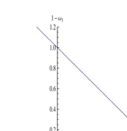
Let us exemplify the interpretation of the spectral density by looking at the two-dimensional case. We then study the extreme behavior of two random variables,Xi,1 andXi,2. The unit simplexS2 ={(ω1, ω2)∈

[0,∞);ω1+ω2 = 1} in Figure 2.1 is then equivalent to the unit inter-val, [0,1], and H is some function of ω ≡ z1

z1+z2 on [0,1]. H may be

decomposed into three spectral densities. The density h = h2,{1,2} on

the interior of the interval,(0,1), describes the dependence between

ex-tremes of the two components Xi,1 and Xi,2. A positive value of h(ω) means that Xi,1 and Xi,2 are both extreme at the pointω. At the point

{ω = 1}the densityh1,{1} describes those events which are extreme only

in the Xi,1-component. It is in fact the point mass of H∗ at ω = 1,

H∗({1}). Analogously, h₁_,{2} is the density at {ω = 0} and the point

mass of H∗ at ω = 0, H∗({0}). It describes those events which are

ex-treme only inXi,2. Since by Equation (2.10) the total mass ofH∗ onS2 is two, we have

H∗(S2) =

Z 1

0

(17)

-0.2 0.2 0.4 0.6 0.8 1.0 1.2 Ω1 -0.2 0.2 0.4 0.6 0.8 1.0 1.2 1-Ω1

Figure 2.1: Unit simplex in two dimensions 2.3.2 Pickands dependence function

An alternative measure of dependence between extremes in the two-dimensional case is the Pickands dependence function A. It is dened

as

A(t) =l(1−t, t) (2.13)

for t ∈ [0,1], where l is the stable tail dependence function dened in

Equation (2.7).

The stable tail dependence function is uniquely determined by its cor-responding Pickands dependence function, since it follows from Equation (2.7) that l(v1, v2) = (v1+v2)A v2 v1+v2 ,

where 0 ≤v1, v2 <∞ and v1+v2 >0. Because of properties 2, 3 and 4 of the stable tail dependence function expressed in Chapter 2.2, the Pickands dependence function possesses the following properties:

• A(0) =A(1) = 1

(18)

• A is convex

IfAassumes its lower bound,A(t) = (1−t)∨t, we have complete

depen-dence. IfA assumes its upper bound, A(t) = 1, we have independence.

An A in between its lower and upper bound corresponds to some other

type of dependence.

From Equation (2.7) we have the following relation between a multi-variate extreme value distribution function with standard Fréchet mar-gins,G∗, and its corresponding Pickands dependence function:

G∗(z1, z2) = exp − 1 z1 + 1 z2 A z1 z1+z2 . (2.14)

(19)

3 Parametric families for bivariate extreme value

distributions

As mentioned in Chapter 2.2, there is in general no nite parametriza-tion for multivariate extreme value distribuparametriza-tions. However, a number of parametric subfamilies have been developed. Gumbel (1960) was the rst to construct parametric models for bivariate extremes. Here we give a review of the most common existing dierentiable parametric families for bivariate extremes. Information about, and a visual understanding of the dependence structure is gained with a transformation to the spectral measure as described in Chapter 2.3.1. We will use the notation from the same chapter. We let (X1, X2) be a bivariate random variable and

G∗ the corresponding bivariate extreme value distribution function with

standard Fréchet margins, describing the extreme behavior of X1 and

X2.

3.1 Independence and complete dependence The distribution function

G∗(z1, z2) = exp − 1 z1 + 1 z2 = exp −1 z1 exp −1 z2 , (3.1)

corresponds to independence. Thus, extreme events in X1 andX2 occur independently. In the two-dimensional unit simplexS2, this corresponds

to zero spectral density on(0,1), h(ω) =h z1 z1+z2 =−(z1+z2)3 ∂V∗ ∂z1∂z2 (z1, z2) =−(z1+z2)3·0 = 0.

The spectral mass at the endpoint ω= 1 describes events extreme only

inX1, H∗({1}) =h₁_,{1} =− lim z2→0 z₁2∂V∗ ∂z1 (z1, z2) =−z12 −1 z₁2 = 1,

while the mass at the other endpoint, ω = 0, describes events extreme

only in X2, H∗({0}) =h1,{2} =− lim z1→0 z₂2∂V∗ ∂z2 (z1, z2) =−z22 −1 z2 2 = 1.

(20)

Thus, independence corresponds to point masses at the endpoints. Note that the total mass is 2, which is consistent with Equation (2.10).

For two completely dependent variables, i.e. P(X1 = X2) = 1, the distribution function is G∗(z1, z2) = exp −min 1 z1 , 1 z2 .

Here all the mass of H∗ is at the point ω = z1

z1+z2 = 1/2, corresponding

to extreme values of X1=X2. Thus, H∗({1₂}) =H∗(S2) = 2. 3.2 Logistic distribution

The logistic model was developed by Tawn (1988). Its distribution func-tion is G∗(z1, z2) (3.2) = exp ( − 1−ψ1 z1 +1−ψ2 z2 + ( ψ1 z1 1/α + ψ2 z2 1/α)α!) ,

where0≤ψ1, ψ2 ≤1and α∈(0,1). The spectral density on(0,1)is

h(ω) (3.3) = 1−α α (ψ1ψ2) 1/α_{_ω₍₁₋_ω_)}−1/α−1_[_ψ1/α 1 ω −1/α₊_ψ1/α 2 (1−ω) −1/α_]α−2_.

Let us also look at the endpoints of the interval. The mass atω= 1 is

H∗({1}) =− lim z2→0 z₁2∂V∗ ∂z1 (z1, z2) = 1−ψ1, and at ω= 0 H∗({0}) =− lim z1→0 z₂2∂V∗ ∂z2 (z1, z2) = 1−ψ2.

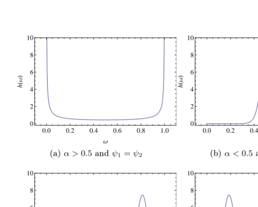
Thus, there is mass at the endpoints as well as in the interior of the inter-val, corresponding to events extreme in only one variable or in both, re-spectively. By varying the parametersα,ψ1andψ2, the spectral density takes on dierent shapes, corresponding to dierent dependence struc-tures. The spectral density always has one peak (for α < 0.5) or one

(21)

0.0 0.2 0.4 0.6 0.8 1.0 0 2 4 6 8 10 Ω h H Ω L (a)α >0.5andψ1=ψ2 0.0 0.2 0.4 0.6 0.8 1.0 0 2 4 6 8 10 Ω h H Ω L (b)α <0.5andψ1=ψ2 0.0 0.2 0.4 0.6 0.8 1.0 0 2 4 6 8 10 Ω h H Ω L (c)α <0.5andψ1> ψ2 0.0 0.2 0.4 0.6 0.8 1.0 0 2 4 6 8 10 Ω h H Ω L (d)α <0.5andψ1< ψ2

(22)

dip (for α > 0.5). As α increases, there is a gradual transformation

from peak to dip around α = 0.5. The parameter α may be seen as

a dependence parameter which determines the shape of the peak. The smaller the α, the higher and narrower the peak, corresponding to more

dependence. In the limit α → 0 the logistic model becomes the

com-plete dependence model. Figure 3.1b shows the spectral measure for near-complete dependence. The mass is here centered around ω = 0.5,

corresponding to X1 and X2 being extreme at the same time. As α in-creases, the spectral mass ows towards the endpoints, corresponding to more independence. In the limitα→1withψ1 =ψ2, the logistic model becomes the independence model. Figure 3.1a shows the spectral mea-sure for a near-independence situation. The mass is concentrated at the endpoints of the interval, representing two separate extreme behaviors

for X1 and X2. Large values of the parameters ψ1 and ψ2 give a high

peak, corresponding to large dependence. Small values ofψ1andψ2give a smeared out peak with more mass at the endpoints, corresponding to small dependence. They may also be seen as asymmetry parameters. The case ψ1 > ψ2 gives a peak at ω > 0.5, as shown in Figure 3.1c. The case ψ1 < ψ2 gives a peak at ω < 0.5, displayed in Figure 3.1d. For ψ1 = ψ2 = ψ we have a mixture of a symmetric logistic and an independence model, G∗(z1, z2) (3.4) = exp ( − (1−ψ) 1 z1 + 1 z2 +ψ ( 1 z1 1/α + 1 z2 1/α)α!) .

The particular case ψ1 = ψ2 = 1 is called the symmetric logistic distri-bution and corresponds to the distridistri-bution function

G∗(z1, z2) = exp ( − 1 z1 1/α + 1 z2 1/α!α) , (3.5)

(23)

3.3 Negative logistic distribution

Developed by Joe (1990), the distribution function for the negative lo-gistic distribution is G∗(z1, z2) = exp    −1 z1 − 1 z2 + ( ψ1 z1 −α + ψ2 z2 −α)−1/α_  ,

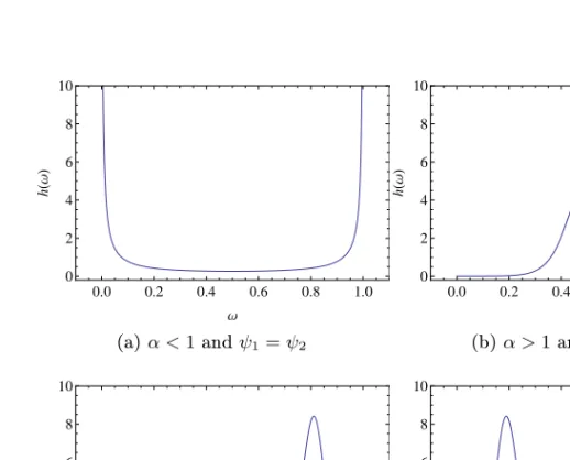
where0≤ψ1, ψ2 ≤1and α >0. The spectral density becomes

h(ω) = (1 +α)ψ₁−αψ₂−α{ω(1−ω)}α−1 ω ψ2 α + ψ1 1−ω α−1/α−2 ,

and is shown for dierent parameter values in Figure 3.2. There is mass at the endpoints as well, since

H∗({1}) =− lim z2→0 z₁2∂V∗ ∂z1 (z1, z2) = 1−ψ1, and H∗({0}) =− lim z1→0 z₂2∂V∗ ∂z2 (z1, z2) = 1−ψ2.

The structure of the negative logistic distribution is similar to that of the logistic distribution. The caseψ1 =ψ2 = 1is symmetric. The limit

α,ψ1 or ψ2 →0 gives the independence model. The case ψ1 =ψ2 = 1 and α→ ∞ gives the complete dependence model.

3.4 Bilogistic distribution

Derived by Joe et al. (1992), the bilogistic distribution function is

G∗(z1, z2) = exp − Z 1 0 max (1−α1)s−α1 z1 ,(1−α2)(1−s) −α2 z2 ds ,

for α1, α2 ∈(0,1]. The spectral density is

h(ω) = (1−α1)(1−z)z

1−α1

(1−ω)ω2_{(1₋_z₎_α

1+zα2}

(24)

0.0 0.2 0.4 0.6 0.8 1.0 0 2 4 6 8 10 Ω h H Ω L (a)α <1andψ1=ψ2 0.0 0.2 0.4 0.6 0.8 1.0 0 2 4 6 8 10 Ω h H Ω L (b)α >1andψ1=ψ2 0.0 0.2 0.4 0.6 0.8 1.0 0 2 4 6 8 10 Ω h H Ω L (c)α >1andψ1> ψ2 0.0 0.2 0.4 0.6 0.8 1.0 0 2 4 6 8 10 Ω h H Ω L (d)α >1andψ1< ψ2

(25)

wherez is the root of

(1−α1)(1−ω)(1−z)α2 −(1−α2)ωzα1 = 0.

There is no spectral mass at the endpoints (H∗({1}) = H∗({0}) = 0).

In some applications this is a reasonable assumption, if there are no ob-servations on the boundary of the sample space. Note that this is not the case for the logistic and negative logistic distributions (except for the symmetric cases ψ1=ψ2=1). The bilogistic distribution is a

gener-alization of the symmetric logistic distribution, since for α1 = α2 the bilogistic distribution reduces to the logistic distribution, seen in gures 3.3a and 3.3b. Generally, α1−α2 ,may be seen as a measure of asymme-try in the dependence structure. Similarly, α1+α2 measures the extent of dependence. Forα1, α2 →1we have independence, and forα1, α2→0 complete dependence.

3.5 Dirichlet extreme value distribution

The Dirichlet distribution, also known as the Beta extreme value dis-tribution, was derived by Coles and Tawn (1991). Its joint distribution function is G∗(z1, z2) = exp{− 1 z1 1−Be α1+ 1, α2; α1z1 α1z1+α2z2 − 1 z2 Be α1, α2+ 1; α1z1 α1z1+α2z2 }, whereα1, α2 >0 and Be(α1, α2;u) = Γ(α1+α2) Γ(α1)Γ(α2) Z u 0 ωα1−1₍₁₋_ω₎α2−1_dω

is a normalized incomplete beta function. The spectral density on(0,1)

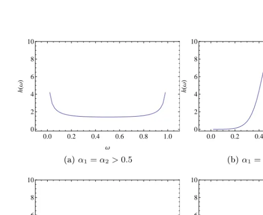
is h(ω) = α α1 1 α α2 2 Γ(α1+α2+ 1) Γ(α1)Γ(α2) ωα1−1₍₁₋_ω₎α2−1 α1ω+α2(1−ω)1+α1+α2 ,

and is shown for dierent parameter values in Figure 3.4. As for the bil-ogistic distribution, there is no mass at the endpoints, since H∗({1}) =

(26)

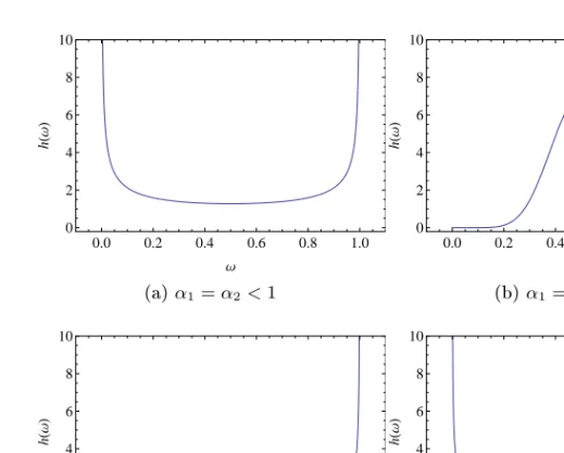
0.0 0.2 0.4 0.6 0.8 1.0 0 2 4 6 8 10 Ω h H Ω L (a)α1=α2>0.5 0.0 0.2 0.4 0.6 0.8 1.0 0 2 4 6 8 10 Ω h H Ω L (b)α1=α2<0.5 0.0 0.2 0.4 0.6 0.8 1.0 0 2 4 6 8 10 Ω h H Ω L (c)α1> α2 0.0 0.2 0.4 0.6 0.8 1.0 0 2 4 6 8 10 Ω h H Ω L (d)α1< α2

(27)

0.0 0.2 0.4 0.6 0.8 1.0 0 2 4 6 8 10 Ω h H Ω L (a)α1=α2<1 0.0 0.2 0.4 0.6 0.8 1.0 0 2 4 6 8 10 Ω h H Ω L (b)α1=α2>1 0.0 0.2 0.4 0.6 0.8 1.0 0 2 4 6 8 10 Ω h H Ω L (c)α1> α2 0.0 0.2 0.4 0.6 0.8 1.0 0 2 4 6 8 10 Ω h H Ω L (d)α1< α2

Figure 3.4: Spectral density for the Dirichlet distribution

H∗({0}) = 0. The parameter combination α1−α2

2 is a measure of asym-metry. Forα1 =α2 we have symmetry. Similarly, α1+₂α2 is a measure of dependence. The limit α1, α2 →0 gives independence, andα1, α2 → ∞ complete dependence.

(28)

4 Stable mixture models

In this chapter we introduce a class of stable mixture models. The mod-els were introduced separately by Watson and Smith (1985) as tensile strength models and by Hougaard (1986) and Crowder (1989) in a sur-vival analysis context. They have since been applied and further devel-oped in Tawn (1990) in a study of extreme sea levels, in Crowder (1998) in survival analysis and in Fougères et al. (2009) with an application to pitting corrosion.

In Chapter 4.1 we give three dierent physical interpretations of the mixture models. In Chapter 4.2 we introduce a class of stable mixture models. We show their diversity in Chapter 4.3 by proving that their distribution functions are dense in the set of all multivariate extreme value distribution functions. We present the results for Fréchet distribu-tions. The results for Gumbel and Weibull distributions are analogous and mentioned in Chapter 5.7.

We start by lettingS be a positive stable random variable

character-ized by its Laplace transform

E[e−tS] =e−tα, t≥0. (4.1)

whereα∈(0,1]. In the terminology of Samorodnitsky and Taqqu (1994), S ∼Sα

cosπα₂ 1/α,1,0

. Here c = cosπα₂ 1/α is a scale parameter, β = 1 an asymmetry parameter, µ = 0 a location parameter and α

a stability parameter. The combination β = 1 and µ = 0 gives the

support [0,∞). The stable distribution is heavy-tailed and leptokurtic.

The α parameter species the asymptotic behavior of the distribution.

A smaller α corresponds to a thicker right tail of the distribution.

Now letF be a Fréchet distributed variable with location parameter µ, scale parameter σ >0 and shape parameterγ >0:

P(F ≤x) = exp ( − x−δ σ/γ −1/γ + ) ,

whereδ ≡µ−σ/γis the nite left endpoint of the distribution. Dene a

new variableXby mixing the Fréchet distribution over a positive stable

distribution:

(29)

Conditionally on S, X is then Fréchet distributed with a new scale

pa-rameter Sγσ and the same left endpoint δ: P(X ≤x|S) =P(SγF + (1−Sγ)δ≤x|S) =P F ≤ x−(1−S γ₎_δ Sγ S (4.3) = exp    − x−(1−Sγ₎_δ Sγ −δ σ/γ !−1/γ +    = exp ( − x−δ Sγ_σ/γ −1/γ + ) = exp ( −S x−δ σ/γ −1/γ + ) .

Taking expectations, we get the unconditional distribution of X, P(X≤x) =E[P(X≤x|S)] =E " exp ( −S x−δ σ/γ −1/γ + )# (4.4) = exp ( − x−δ σ/γ −α/γ + ) = exp ( − x−δ σ α/ γ α −1/(γ/α) + ) .

Thus, X is unconditionally also Fréchet distributed, but with a larger

scale parameter σ/αand a larger shape parameterγ/α. We say that F

is directed by S. Note that in the special case δ = 0, σ =γ = α,X is

unconditionally standard Fréchet distributed:

P(X≤x) = exp{−x₊−α/γ}= exp{−x−₊1}. (4.5)

4.1 Interpretations of the stable mixture model

The stable mixture model may be interpreted physically in a number of ways. We give three dierent interpretations. The interpretations are inspired by Fougères et al. (2009), who give interpretations for Gumbel stable mixture models.

4.1.1 Fréchet distribution as a scale mixture of Fréchet distri-butions

LetF ∼GEV(µ, σ1, γ >0) be a Fréchet distributed variable and look at the following mixture variable,

(30)

whereσ2 >0is some constant. The conditional distribution ofXis then P(X≤x|S) =P(σ2SγF+ (1−σ2Sγ)δ≤x|S) =P F ≤ x−(1−σ2S γ₎_δ σ2Sγ S = exp    − x−(1−σ2Sγ)δ σ2Sγ −δ σ1/γ !−1/γ +    = exp ( − x−δ Sγ_σ 1σ2/γ −1/γ + ) = exp ( −S x−δ σ1σ2/γ −1/γ + ) .

Taking expectations, we get the unconditional distribution,

P(X≤x) =E[P(X ≤x|S)] =E " exp ( −S x−δ σ1σ2/γ −1/γ + )# (4.6) = exp ( − x−δ σ1σ2/γ −α/γ + ) = exp ( − x−δ σ1σ2 α / γ α −1/(γ/α) + ) .

Thus, the unconditional distribution of X is Fréchet distributed with a

new scale parameter σ1σ2/α and a new shape parameter γ/α. The left endpoint δ is unchanged. This corresponds to a scale transformation

with an accompanying shape and location transformation. To interpret this physically, consider an area consisting of a number of groups. Each group has its own Fréchet variation (with parameters µ, σ1, γ > 0) of some variable of interest. On top of the Fréchet variation there is an additional variation aecting all the groups in the area. This additional variation has a stable distribution with parameter α. The unconditional

distribution in a test area is described by Equation (4.6).

4.1.2 Fréchet distribution as a size mixture of Fréchet distri-butions

Here we regard an area consisting of ngroups, all of the same size. The

maximum value of the variable of interest in each group is GEV(µ, σ1, γ >

0)-distributed. The maximum value (≡X) of the variable in the whole

area then has distribution function

P(X ≤x) = exp ( − x−δ σ1/γ −1/γ + )!n = exp ( −n x−δ σ1/γ −1/γ + ) .

(31)

If we assume that the size of the area is non-integer and random, we can replacen withSσ₂1/γ. Then

P(X≤x|S) = exp ( −Sσ₂1/γ x−δ σ1/γ −1/γ + ) = exp ( −S x−δ σ1σ2/γ −1/γ + ) , and P(X≤x) = exp ( − x−δ σ1σ2/γ −1/(γ/α) + ) .

With this interpretation,Sσ₂1/γ is the random size of the area under the

inuence of some external factor.

4.1.3 Fréchet distribution as the maximum of a conditional Poisson point process

Let X1, X2, ... be iid variables. Then (see e.g. Leadbetter et al., 1983) there exist sequences of constants {cn} and {dn>0}such that

P Mn−cn dn ≤x →exp ( − x−δ σ1/γ −1/γ + ) ,

whereδ =µ−σ1/γ, if and only if the point process

Nn= i n+ 1, Xi−cn dn :i= 1, ..., n

converges to a certain Poisson processN on regions of the form(0,1)× [u,∞) for anyu > δ;

Nn→N.

The Poisson point process N has intensity measure Λ, which for A = [t1, t2]×[x,∞), witht1, t2∈(0,1)andt1 < t2, is given by

Λ(A) = (t2−t1) x−δ σ1/γ −1/γ .

(32)

If we include a random term Sσ21/γ in the intensity, Λ(A) = (t2−t1)Sσ21/γ x−δ σ1/γ −1/γ = (t2−t1) x−δ Sγ_σ 1σ2/γ −1/γ , then equivalently, X ≡ Mn−cn

dn depends on nand is Fréchet distributed

conditionally on S: P(X≤x|S) =P Mn−cn dn ≤x|S →exp ( − x−δ Sγ_σ 1σ2/γ −1/γ + ) = exp ( −S x−δ σ1σ2/γ −1/γ + ) .

Thus, X is Fréchet distributed with scale parameter σ1σ2/α, shape pa-rameter γ/αand left endpoint δ,

P(X≤x) =E[P(X≤x|S)] = exp ( − x−δ σ1σ2/γ −1/(γ/α) + ) = exp ( − x−δ σ1σ2 α / γ α −1/(γ/α) + ) .

4.2 A class of stable mixture models

In this chapter we introduce a class of multivariate stable mixture mod-els. They may be seen as an extension of the univariate stable mixture model in Equation (4.2) with left endpointδ set to zero for convenience.

Let {Si;i = 1, ..., n} be independent positive stable variables dened in Equation (4.1). Also let {Fj}, j = 1, ..., d, be independent Fréchet variables with distribution functionsexp

− 1

x1+/α

. Now create mixture variables by mixing each Fréchet variable overnpositive stable

distribu-tions: Xj = n X i=1 cj,iSi !α Fj (4.7)

(33)

for j= 1, ..., dand constants cj,i ≥0. Then the conditional distribution of Xj given the stable variables is

P(Xj ≤xj|Si, i= 1, ..., n) = exp ( − n X i=1 cj,iSi 1 x1_j/α ) . (4.8)

Taking expectations, we get the joint distribution function for the stable mixture: Gn(x)≡P(X≤x) =E[P(X≤x|Si, i= 1, ..., n)] (4.9) =E[P(X1≤x1|Si, i= 1, ..., n)·...·P(Xd≤xd|Si, i= 1, ..., n)] =E " exp ( − n X i=1 c1,iSi 1 x1₁/α ) ·...·exp ( − n X i=1 cd,iSi 1 x1_d/α )# =E " _n Y i=1 exp ( − c1,i 1 x1₁/α +...+cd,i 1 x1_d/α ! Si )# = n Y i=1 exp ( − c1,i 1 x1₁/α+...+cd,i 1 x1_d/α !α) = exp ( − n X i=1 c1,i 1 x1₁/α +...+cd,i 1 x1_d/α !α) .

Let us check if Gn is an extreme value distribution function, or equiva-lently, if Gn is max-stable (see Equation (2.3)). Thus, we need to nd

d-dimensional vectors of constants Am >0 and Bm such that for every

m= 2,3, ...

(34)

Starting from the right-hand side, Gm_n(Am,1x1+Bm,1, ..., Am,dxd+Bm,d) = exp    − n X i=1   d X j=1 cj,i 1 (Am,jxj+Bm,j)1/α   α m    = exp    − n X i=1   d X j=1 cj,i m1/α (Am,jxj+Bm,j)1/α   α   = exp    − n X i=1   d X j=1 cj,i 1 Am,j m1/αxj + Bm,j m1/α !1/α  α   .

Now, if we letAm,1 =...=Am,d=m1/α and Bm =0 we have Equation (4.10). This means that the distribution function Gn is max-stable and thus an extreme value distribution function. For convenience we will work with standard Fréchet marginals, which is the case if

n

X

i=1

cα_j,i = 1for all j= 1, ..., d. (4.11)

Let us look at the dependence structure for our stable mixture models. For simplicity we start withd= 2dimensions. The distribution function

is then Gn(x1, x2) = exp ( − n X i=1 c1,i 1 x1₁/α +c2,i 1 x1₂/α !α) .

The spectral density is calculated with Equation (2.12):

h x1 x1+x2 =−(x1+x2)3 ∂V∗ ∂x1∂x2 (x1, x2) =−(x1+x2)3 n X i=1 α−1 α c1,ic2,i c1,i 1 x1₁/α +c2,i 1 x1₂/α !α−2 ·x−₁1/α−1x−₂1/α−1.

(35)

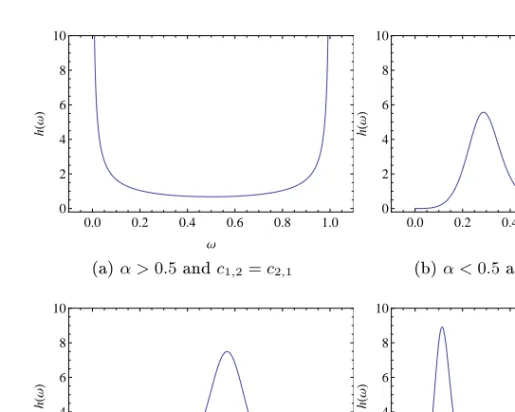
0.0 0.2 0.4 0.6 0.8 1.0 0 2 4 6 8 10 Ω h H Ω L (a)α >0.5andc1,2=c2,1 0.0 0.2 0.4 0.6 0.8 1.0 0 2 4 6 8 10 Ω h H Ω L (b)α <0.5andc1,2=c2,1 0.0 0.2 0.4 0.6 0.8 1.0 0 2 4 6 8 10 Ω h H Ω L (c)α <0.5,c1,1> c1,2, c2,1> c2,2 0.0 0.2 0.4 0.6 0.8 1.0 0 2 4 6 8 10 Ω h H Ω L (d)α <0.5,c1,1> c1,2, c2,1< c2,2

Figure 4.1: Spectral density for stable mixtures in two dimensions A change of variables r=x1+x2 andω= _x₁x₊1_x₂ gives

h(ω) =r3 n X i=1 1−α α c1,ic2,i c1,i 1 (rω)1/α +c2,i 1 (r(1−ω))1/α α−2 ·(rω)−1/α−1(r(1−ω))−1/α−1 = n X i=1 1−α α c1,ic2,i c1,i 1 ω1/α +c2,i 1 (1−ω)1/α α−2 ·(ω(1−ω))−1/α−1.

Forn= 1 this is the symmetric logistic distribution in Equation (3.5).

For n≥2 we have a product of logistic distributions in Equation (3.3)

(36)

another because of the constraints (4.11). For eachi, there is a peak (for α <0.5) or a dip (forα >0.5). A smallαgives high peaks, corresponding

to large dependence. The explanation is that a smallαgives a thick right

tail in the density of the stable variableS, which then is a dominant factor

in extremes of X (dened in Equation (4.7)). By varying the parameters

α andcj,i,j= 1, ..., d,i= 1, ..., n, we get dierent shapes of the spectral density, corresponding to dierent dependence structures. Figure 4.1 shows the spectral density in two dimensions for some parameter values. Now we pose the question; may any dependence structure be achieved this way? We are interested in how big this subfamily of multivariate extreme value distributions is. If this family of stable mixture distribu-tions is in fact the entire class of multivariate extreme value distribudistribu-tions, then equivalently any multivariate extreme value distribution functionG

may be approximated by a stable mixture distribution functionGn. We would thus have a parametrization for all multivariate extreme value distributions.

We will prove that the set of stable mixture distribution functions

Gn is in fact dense in the set of multivariate extreme value distribution functionsG. First we prove that the set of stable tail dependence

func-tions for stable mixtures is dense in the set of stable tail dependence functions for all multivariate extremes. The following theorem (4.1) im-plies that for any xed vector v, a stable tail dependence function for an extreme value distribution may be uniformly approximated by a stable tail dependence function for a stable mixture.

4.3 A density theorem

In this section we prove that the set of stable tail dependence functions for the family of stable mixtures in Equation (4.7) is dense in the set of all stable tail dependence functions for multivariate extreme value distributions. As any multivariate extreme value distribution can be transformed to a distribution with standard Fréchet margins, we assume standard Fréchet margins throughout.

Recall from Equation (2.8) the stable tail dependence functionl for

(37)

H∗, l(v) = Z Sd d _ j=1 (ωjvj)H∗(dω), (4.12) and the constraint on H∗ of standard Fréchet margins from Equation

(2.9)

Z

Sd

ωjH∗(dω) = 1, (4.13)

for all j= 1, ..., d.

Now letln be the stable tail dependence function for the stable mix-ture variable (4.7) with distribution function Gn from Equation (4.9),

ln(v) =−logGn 1 v1 , ..., 1 vd = n X i=1 c1,iv11/α+...+cd,iv1d/α α ,(4.14)

for v∈[0,∞]. For the stable mixture, the standard Fréchet constraint

reads

n

X

i=1

cα_j,i = 1for all j= 1, ..., d, (4.15)

from Equation (4.11).

Theorem 4.1. Let l be as in (4.12) and V any positive d-dimensional

vector. Let >0. Then there exists anN ∈Nsuch that for all v∈[0,V]

and n≥N, there exists some ln as in (4.14) with

|l(v)−ln(v)|< .

We will approximate a general multivariate extreme value stable tail dependence function,l, with a stable tail dependence function for a stable

mixture, ln, in a series of steps. In the rst two steps we approximate

l(v)with a sum. In the third step we normalize constants in this sum in

a way to satisfy the standard Fréchet marginal condition (4.15). Finally we use the triangle equality several times.

(38)

We start by approximating the integral in (4.12) with a sum. Further,

we partition the d-dimensional unit simplex Sd into subareas Ωi, i =

1, ..., n, small enough so that

diam(Ωi) = sup(d(x, y);x, y∈Ωi)< d,

where dis the Euclidean distance andd>0 depends on n and will be specied later. For each i, choose a pointωi inΩi.

Lemma 4.2. Let > 0. Then there exists N ∈ _N such that for all

v∈[0,V] andn≥N, R Sd Wd j=1ωjvj H∗(dω)−Pn i=1 Wd j=1ωijvj H∗(Ωi) < /3.

Proof. The total mass of H∗ isd (H∗(Sd) = d) because of the standard Fréchet condition (4.13). We will use this in the second to last step below. In the third to last step we use thatω∈[0,1], and then get that

Z Sd   d _ j=1 ωjvj  H∗(dω)− n X i=1   d _ j=1 (ωi_jvj  H∗(Ωi) ≤ n X i=1 Z Ωi   d _ j=1 ωjvj  H∗(dω)−   d _ j=1 ωi_jvj  H∗(Ωi) ≤ n X i=1  max Ωi   d _ j=1 ωjvj  −   d _ j=1 ωi_jvj    H∗(Ωi) ≤ n X i=1 d   d _ j=1 vj  H∗(Ωi) =d   d _ j=1 vj  d≤d   d _ j=1 Vj  d.

Finally, if we choosed small enough (that isnlarge enough) so that

d   d _ j=1 Vj  d < /3⇔d< /3 Wd j=1(Vj)d , (4.16)

the result follows.

In the next step we approximate the maximum-function in Lemma 4.2 with a sum.

(39)

Lemma 4.3. Let > 0. Then there exists an N ∈_N and an α ∈(0,1]

such that for all v∈[0,V]andn≥N, n X i=1   d _ j=1 ω_jivj  H∗(Ωi)− n X i=1 ωi₁v1 1/α +...+ ω_divd 1/αα H∗(Ωi) < /3.

Proof. We use that for any constant a ≥0 and any α ∈ (0,1] we have a₁1/α+...+a_d1/αα≤dαWd j=1aj, | n X i=1 ωi₁v1 1/α +...+ ω_divd 1/αα H∗(Ωi)− n X i=1   d _ j=1 ω_jivj  H∗(Ω_i)| = n X i=1   ω₁iv1 1/α +...+ ω_divd 1/αα −   d _ j=1 ωi_jvj    H∗(Ω_i) ≤ n X i=1      d   d _ j=1 ωi_jvj   1/α   α −   d _ j=1 ω_jivj     H∗(Ωi) = n X i=1   d _ j=1 ω_jivj  (dα−1)H∗(Ω_i)≤ n X i=1 H∗(Ωi)   d _ j=1 vj  (dα−1) =d   d _ j=1 vj  (dα−1)≤d   d _ j=1 Vj  (dα−1).

If we choose α small enough such that d   d _ j=1 Vj  (dα−1)< /3⇔dα <1 + /3 dWd j=1Vj , (4.17) Lemma 4.3 follows.

We want to nd constantscj,i for j = 1, ..., d and i= 1, ..., n in the expression (4.14) for the stable tail dependence function for our stable

(40)

mixture that fulll the standard Fréchet condition (4.11). Therefore, we normalize the constants(ω_jiH∗(Ωi))1/αfrom Lemma 4.3 by dening

cj,i≡ ωi_jH∗(Ωi) Pn m=1ωmj H∗(Ωm) !1/α , for j= 1, ..., d,i= 1, ..., nand α∈(0,1].

Lemma 4.4. Let > 0. Then there exists an N ∈_N and an α ∈(0,1]

such that for all v∈[0,V]andn≥N, | n X i=1 ωi₁v1 1/α +...+ ω_divd 1/αα H∗(Ωi) − n X i=1 c1,iv1₁/α+...+cd,iv 1/α d α |< /3.

Proof. We use the requirement (4.13) onH∗, n X i=1 ω_jiH∗(Ωi)−1 = n X i=1 ω_jiH∗(Ωi)− Z Sd ωjH∗(dω) ≤ n X i=1 max Ωi ωj−ωji H∗(Ωi)≤ n X i=1 dH∗(Ωi) =dd,

(41)

and get | n X i=1 ω₁iv1 1/α +...+ ωi_dvd 1/αα H∗(Ωi) − n X i=1 c1,iv₁1/α+...+cd,iv 1/α d α | ≤ n X i=1 ω₁iv1 1/α +...+ ωi_dvd 1/αα H∗(Ωi) − ω₁iv1 Pn m=1ω1mH∗(Ωm) 1/α +...+ ω_divd Pn m=1ωdmH∗(Ωm) 1/α!α H∗(Ωi) ≤ n X i=1 ωi₁v1 1/α +...+ ω_divd 1/αα H∗(Ωi) 1 1−dd −1 ≤ n X i=1   d   d _ j=1 vj   1/α   α H∗(Ωi) 1 1−dd −1 =dα d _ j=1 vjd dd 1−dd ≤dαd d _ j=1 Vj dd 1−dd .

If we use the restriction (4.17) onαfrom Lemma 4.3 and choosedsmall enough (i.e. nlarge enough) such that

dαd d _ j=1 Vj dd 1−dd < /3⇔ 1 + /3 dWn j=1Vj ! d d _ j=1 Vjdd < 3(1−dd) ⇔(d n _ j=1 Vj+/3)dd < 3− 3dd⇔d< /3 d2Wn j=1Vj+2₃d ,

Lemma 4.4 follows. This is a stronger restriction on d than (4.16) from Lemma 4.2. Alternatively, we can use (4.16) ondand restrictα instead

(42)

of d: dαd d _ j=1 Vj 1 1−dd −1 < /3⇒dαd d _ j=1 Vj    1 1−Wd/3 j=1Vj −1   < /3 ⇔dαd d _ j=1 Vj /3 Wd j=1Vj−/3 < /3⇔dα< Wd j=1Vj−/3 dWd j=1Vj .

This is a stronger restriction on α than (4.17).

Now we are ready to prove our theorem.

Proof of Theorem 4.1. We use Lemmas 4.2-4.4 and the triangle inequal-ity: |l(v)−ln(v)|= Z Sd d _ j=1 (ωjvj)H∗(dω)− n X i=1 c1,iv 1/α 1 +...+cd,iv 1/α d α ≤ Z Sd d _ j=1 (ωjvj)H∗(dω)− n X i=1 d _ j=1 (ωi_jvj)H∗(Ωi) + n X i=1 d _ j=1 (ωi_jvj)H∗(Ωi)− n X i=1 (ω₁iv1)1/α+...+ (ωidvd)1/α α H∗(Ωi) + n X i=1 (ω₁iv1)1/α+...+ (ωidvd)1/α α H∗(Ωi) − n X i=1 c1,iv1₁/α+...+cd,iv 1/α d α < /3 +/3 +/3 =

Theorem 4.1 says that the stable tail dependence function for any extreme value distribution may be uniformly approximated by the sta-ble tail dependence function for a stasta-ble mixture on an interval [0,∞).

In this section we show that the same can be done for the respective distribution functions G(x) =e−l(1/x) and Gn(x) =e−ln(1/x).

(43)

Theorem 4.5. Let G be a d-dimensional extreme value distribution

function. Then for every G > 0 there exists an n ∈ N and a

distri-bution function Gn for a d-dimensional stable mixture, such that for all x∈[0,∞],

|Gn(x)−G(x)|< G.

Proof. Note that because we assume standard Fréchet marginals, we

have G(x) = Gn(x) = 0 for x∈[0,∞). We let γ be a constant vector

and consider the cases x∈[0,∞)\[0,γ]and x∈[0,γ]separately.

Assuming thatln(1_x)−l(_x1) is small, we can use Taylors formula on

exp{ln(_x1)−l(1_x)}. We also use Theorem 4.1 where we let=G/6and

V = 1/γ. Then for x∈[0,∞)\[0,γ]andln(1_x)−l(_x1)small

|Gn(x)−G(x)|= e −ln(1_x)₋_e−l(1_x) =e −ln(1_x) 1−e ln(1_x)−l(1_x) ≤e−ln(_x1) 2 ln 1 x −l 1 x <1·2=G/3. For x∈[0,γ]we use the non-decreasing quality of the distribution

func-tion G. By choosing γ small enough, G(γ) can be made smaller than G/3. By above we have |Gn(x)−G(x)|< G/3 and get

|Gn(x)−G(x)| ≤Gn(x) +G(x)≤Gn(γ) +G(γ)

≤ |Gn(γ)−G(γ) + 2G(γ)|

(44)

5 Some stable mixtures models

In this section we study a number of stable mixture models of the class presented in Equation (4.7). We investigate their dependence structures via a transformation to the spectral measure. The results are presented for Fréchet distributions. However, the models are easily transferable to Gumbel and Weibull distributions, as will be described in Chapter 5.7.

LetT andAbe discrete index sets, andTnite. Also let{ct,a},t∈T,

a ∈ A, be non-negative constants and {Sa}, a ∈ A, be independent positive α-stable variables dened by Equation (4.1). We look at the

following T-dimensional stable mixture model, Xt= X a∈A ct,aSa !γ Ft+ 1− X a∈A ct,aSa !γ! δt, (5.1)

where t ∈ T, δt = µt−σt/γ, Ft ∼GEV(µt, σt, γ > 0), and Ft and Sa are all mutually independent. The distribution ofXt conditioned on the stable variables is P(Xt≤xt|Sa, a∈A) =P X a∈A ct,aSa !γ Ft+ 1− X a∈A ct,aSa !γ! δt≤xt|Sa, a∈A ! =P Ft≤ xt− 1− P_a∈Act,aSa γ δt P a∈Act,aSa γ ! = exp        −    xt−(1−(Pa∈Act,aSa) γ )δt (P a∈Act,aSa) γ −δ_t σt/γ    −1/γ +        = exp    − xt−δt σt/γ Pa∈Act,aSa γ !−1/γ +    = exp ( −(X a∈A ct,aSa) xt−δt σt/γ −1/γ + ) .

Thus, theXt's are conditionally independent Fréchet variables with scale parameters σt P_a∈Act,aSa

γ

(45)

X={Xt}t∈T is P(Xt≤xt, t∈T) =E[P(Xt≤xt, t∈T|Sa, a∈A)] (5.2) =E " Y t∈T P(Xt≤xt|Sa, a∈A) # =E " Y t∈T exp ( −(X a∈A ct,aSa) xt−δt σt/γ −1/γ + )# =E " Y t∈T Y a∈A exp ( −ct,aSa xt−δt σt/γ −1/γ + )# =E " Y a∈A exp ( −X t∈T ct,aSa xt−δt σt/γ −1/γ + )# = Y a∈A E " exp ( −Sa X t∈T ct,a xt−δt σt/γ −1/γ + )# = Y a∈A exp ( − X t∈T ct,a xt−δt σt/γ −1/γ + !α) .

By Equation (2.3), X is max-stable if for every m = 2,3, ... there exist

vectors of constants Am >0 and Bm such that

P(Xt≤xt, t∈T) =P(Xt≤Am,txt+Bm,t, t∈T)m. We start from the right-hand side,

P(Xt≤Am,txt+Bm,t, t∈T)m = Y a∈A exp ( −m X t∈T ct,a Am,txt+Bm,t−δt σt/γ −1/γ + !α) = Y a∈A exp ( − X t∈T ct,am1/α Am,txt+Bm,t−δt σt/γ −1/γ + !α) = Y a∈A exp ( − X t∈T ct,a Am,txt+Bm,t−δt (σt/γ)mγ/α −1/γ + !α) .

By choosing Am,t = mγ/α and Bm,t = δt(1−mγ/α) for all t ∈ T, we see that we have max-stability. Hence, X follows a multivariate extreme

(46)

value distribution. Using the dependence structure tools described in Chapter 2.3.1 and the parametric families from Chapter 3 we will study the dependence of a number of models of the form (5.1). For simplicity we work with standard Fréchet variables, Ft∼GEV(µt = 1, σt = 1, γ = 1). We assume throughout that x≥0.

5.1 One-way random eects model

We start by studying the following one-way random eects model:

Xi,j =SiFi,j, 1≤i≤m,1≤j≤ni,

where Fi,j is standard Fréchet and all variables independent. If we set the index sets to T ={(i, j); 1≤i≤m,1≤j≤ni}and A={1, ..., m}, we have the model (5.1) with ct,a=c(i,j),a = 1{i=a}. By Equation (5.2),

the joint distribution is

P(Xi,j ≤xi,j,(i, j)∈T) = m Y a=1 exp    −   X (i,j)∈T c(i,j),a 1 xi,j   α   = m Y a=1 exp    −   ni X j=1 1 xa,j   α   .

Let us study the dependence between variables at two adjacent points. For two consecutive points in i-space,

P(Xi,j ≤xi,j, Xi+1,j ≤xi+1,j) = i+1 Y a=i exp ( − 1 xα a,j ) = exp ( − 1 xα_i,j ) exp ( − 1 xα_i₊₁_,j ) = exp ( − 1 xα_i,j + 1 xα_i₊₁_,j !) .

Next we standardize the margins to standard Fréchet in order to isolate the dependence structure from the marginal behavior. Using Equation (2.4) we get

G∗(zi,j, zi+1,j) =G(z_i,j1/α, z1_i₊₁/α_,j) = exp

− 1 zi,j + 1 zi+1,j .

(47)

This is the independence model (3.1); sinceSi andSi+1are independent, as are Fi,j and Fi+1,j, Xi,j =SiFi,j and Xi+1,j =SiFi+1,j are naturally independent.

Similarly, for two consecutive points inj-space,

P(Xi,j ≤xi,j, Xi,j+1≤xi,j+1) = exp

   −   j+1 X l=j 1 xa,l   α   = exp − 1 xi,j + 1 xi,j+1 α .

Again transforming to a distribution function G∗ with standard Fréchet

margins gives

G∗(zi,j, zi,j+1) =G(zi,j1/α, z 1/α i,j+1) = exp ( − 1 z_i,j1/α + 1 z1_i,j/α₊₁ !α) .

This is the symmetric logistic model (3.5). For decreasing parameterα,

the variable Si is more dominant inXi,j =SiFi,j and Xi,j+1=SiFi,j+1, giving larger dependence.

Next we study a class of time series models of the formXt=HtγFt+

(1−H_tγ)δt, where we have set δt= 0 andγ = 1 for convenience, i.e. we work with standard Fréchet variables. We let Ht= P∞i=−∞biSt−i be a linear stable process, where theSiare independent stable variables,biare nonnegative constants andHtconverges in distribution ifP∞_i₌₁bαi <∞.

5.2 AR(1) model

We study the following autoregressive time series model,

Xt=HtFt,

where Ft is standard Fréchet, 0 < ρ < 1, and Ht = ρHt−1 +St =

P∞

i=0ρiSt−i is a positive stable AR-process. The index sets are here

(48)

1

(1−ρα₎1/αS0, since by the Laplace transform characterization (4.1) ofS,

E " exp ( −t ∞ X i=0 ρiS−i )# = ∞ Y i=0 Eexp−tρiS−i = ∞ Y i=0 exp−tαρiα (5.3) = exp ( −tα ∞ X i=0 ρiα ) = exp − t α (1−ρα₎ =E " exp ( −t 1 1−ρα 1/α S0 )# ,

for any t≥0. We thus have

0 X a=−∞ ct,aSa= ∞ X i=t ρiSt−i =ρt ∞ X i=0 ρiS−i =d ρt (1−ρα₎1/αS0.

So,ct,0=ρt(1−ρα)−1/α,ct,a=ρt−afor t= 1, ..., n anda= 1, ..., t, and

ct,a= 0 otherwise. Ht= ∞ X i=0 ρiSt−i = X a∈A ct,aSa= 0 X a=−∞ ct,aSa+ t X a=1 ct,aSa+ ∞ X a=t+1 ct,aSa d =ρt 1 (1−ρα₎1/αS0+ t X a=1 ρt−aSa+ 0

We get the joint distribution function from Equation (5.2),

P(Xt≤xt,1≤t≤n) = 0 Y a=−∞ exp ( − n X t=1 ct,a 1 xt !α) · n Y a=1 exp ( − n X t=1 ct,a 1 xt !α) _∞ Y a=n+1 exp ( − n X t=1 ct,a 1 xt !α) = exp ( − 1 (1−ρα₎ n X t=1 ρt xt !α) _n Y a=1 exp ( − n X t=a ρt−a1 xt !α)

(49)

The joint distribution of X1 and X2 can then be calculated as P(X1 ≤x1, X2 ≤x2) = exp ( − 1 1−ρα 2 X t=1 ρt xt !α) ₂ Y a=1 exp ( − 2 X t=a ρt−a xt !α) = exp − 1 1−ρα ρ x1 + ρ 2 x2 α exp − ρ0 x1 +ρ 1 x2 α exp − ρ0 x2 α = exp − 1 1−ρα 1 x1 + ρ x2 α − 1 xα 2 .

Hence, because of stationarity of the process Ht, the joint distribution function for any two consecutive points in time, (Xt, Xt+1) (t<n), is

G(xt, xt+1) =P(Xt≤xt, Xt+1 ≤xt+1) (5.4) = exp − 1 1−ρα 1 xt + ρ xt+1 α − 1 xα_t₊₁ .

Transforming to a distribution function G∗ with standard Fréchet

mar-gins, G∗(zt, zt+1) =G z_t1/α (1−ρα₎1/α, z_t1₊₁/α (1−ρα₎1/α ! = exp ( − 1 z_t1/α + ρ z1_t₊₁/α !α −1−ρ α zt+1 ) .

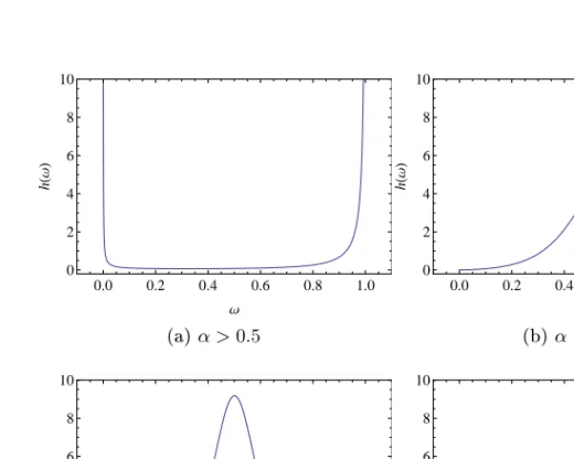
This is the logistic model in Equation (3.2) with parameters ψ1 = 1 and ψ2 = ρα, displayed in Figure 5.1 for dierent values of ρ and α. The AR-process is a dynamic process where the distribution of future values depend on the previous values. More distant values have smaller weights. The parameterρis a measure of strength of memory. Forρ→1

the memory is strong and therefore the dependence large, displayed in Figure 5.1c. Forρ→0memory is weak and therefore dependence small,

as shown in Figure 5.1d. Furthermore, a small α means thicker tails

for the stable variables giving a narrow tall peak. Let us also study the dependence between two points that are m time units apart, Xt and

(50)

0.0 0.2 0.4 0.6 0.8 1.0 0 2 4 6 8 10 Ω h H Ω L (a)α >0.5 0.0 0.2 0.4 0.6 0.8 1.0 0 2 4 6 8 10 Ω h H Ω L (b)α <0.5 0.0 0.2 0.4 0.6 0.8 1.0 0 2 4 6 8 10 Ω h H Ω L (c)α <0.5andρ→1 0.0 0.2 0.4 0.6 0.8 1.0 0 2 4 6 8 10 Ω h H Ω L (d)α <0.5andρ→0

Figure 5.1: Spectral density describing the dependence between two con-secutive points in the AR(1) model

(51)

0.0 0.2 0.4 0.6 0.8 1.0 0 2 4 6 8 10 Ω h H Ω L (a)m= 2 0.0 0.2 0.4 0.6 0.8 1.0 0 2 4 6 8 10 Ω h H Ω L (b)m= 6

Figure 5.2: Spectral density describing the dependence between two points m time points apart in the AR(1) model

with Equation (5.4), G(xt, xt+m) = exp − 1 1−ρα 1 xt + ρ m xt+m α −1−ρ mα 1−ρα 1 xα_t₊_m , giving G∗(zt, zt+m) = exp ( − 1 z_t1/α + ρ m z_t1₊/α_m !α −1−ρ mα zt+m ) .

This is the logistic model with parametersψ1 = 1and ψ2 =ρmα. With increasingm, memory decreases and thus also dependence, as displayed

in Figure 5.2.

5.3 MA(1) model

We have a Fréchet time series model,

Xt=HtFt, (5.5)

whereFtis a standard Fréchet variable, Ht=b0St+b1St−1 is an MA(1) process, andb0, b1 are non-negative constants. Setting the index sets to

(52)

anda={t−1, t}, andct,a= 0otherwise. The joint distribution function is then by (5.2) P(Xt≤xt,1≤t≤n) = n Y a=0 exp    −   n∧(a+1) X t=1∨a bt−a xt   α   .

The joint distribution for the rst two time points is then

P(X1 ≤x1, X2 ≤x2) (5.6) = 2 Y a=0 exp    −   2∧(a+1) X t=1∨a bt−ax−t1   α   = exp ( − 1 X t=1 btx−t1 !α) exp ( − 2 X t=1 bt−1x−t1 !α) ·exp ( − 2 X t=2 bt−2x−t1 !α) = exp − b1 x1 α + b0 x1 + b1 x2 α + b0 x2 α .

By the stationarity of Htwe thus have

G(xt, xt+1) =P(Xt≤xt, Xt+1≤xt+1) = exp − b1 xt α + b0 xt + b1 xt+1 α + b0 xt+1 α .

As before we transfer to a distribution function with standard Fréchet marginals, G∗(zt, zt+1) =G ((bα₀ +bα₁)zt)1/α,((bα0 +bα1)zt+1)1/α (5.7) = exp ( − 1 bα₀ +bα₁ bα₁ zt + b0 z1_t/α + b1 z_t1₊₁/α !α + b α 0 zt+1 !) .

This is the logistic model with ψ1 = b

α 0 bα 0+bα1 and ψ2 = bα1 bα 0+bα1, displayed

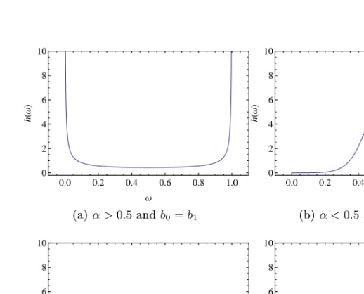
in Figure 5.3. The case b0 > b1, gives a peak in the spectral density for ω > 0.5, as shown in Figure 5.3c. For b0 < b1 we have a peak

(53)

0.0 0.2 0.4 0.6 0.8 1.0 0 2 4 6 8 10 Ω h H Ω L (a)α >0.5andb0=b1 0.0 0.2 0.4 0.6 0.8 1.0 0 2 4 6 8 10 Ω h H Ω L (b)α <0.5andb0=b1 0.0 0.2 0.4 0.6 0.8 1.0 0 2 4 6 8 10 Ω h H Ω L (c)α <0.5andb0> b1 0.0 0.2 0.4 0.6 0.8 1.0 0 2 4 6 8 10 Ω h H Ω L (d)α <0.5andb0< b1

Figure 5.3: Spectral density describing the dependence between two con-secutive points in the MA(1) model

(54)

at ω < 0.5, shown in Figure 5.3d. For b0 = b1 we have a mixture of symmetric logistic and independence, displayed in Figures 5.3a and 5.3b for dierent values ofα.

In order to estimate parameters for a data set tted to the MA(1) model, we would need the likelihood function of the distribution. We look at a general Fréchet variable Ft ∼GEV(µ, σ, γ). We setb0 = 1 for identiability and get

F =P(Xt≤xt,1≤t≤n) (5.8) = n Y k=0 exp    −   n∧(k+1) X t=1∨k bt−k xt−δ σ/γ −1/γ +   α   = exp{− b1 x1−δ σ/γ −1/γ + !α − n−1 X t=1 " xt−δ σ/γ −1/γ + +b1 xt+1−δ σ/γ −1/γ + #α − xn−δ σ/γ −α/γ + } = exp ( −(b1z1)α− n−1 X t=1 (zt+b1zt+1)α−znα ) , wherezt= xt−δ σ/γ −1/γ + fort= 1, ..., n. Deneu1 =b1z1,ut=zt−1+b1zt and un+1 = zn. By induction, the likelihood function can be shown to be L(µ, σ, γ, b1, α|X) =QnF n Y t=1 1 σ xt−δ σ/γ −1/γ−1 + , where Q0= 1 Q1=α(b1uα1−1+u α−1 2 ) Qi=−Qi−2α(α−1)b1uα_i−2+Qi−1α(b1uα_i−1+uα_i₊₁−1), i= 2, ..., n. 5.4 MA(2) model

We have the model

(55)

withFtstandard Fréchet,Ht=b0St+b1St−1+b2St−2an MA(2) process, andb0, b1, b2 non-negative constants. All variables are mutually indepen-dent. SettingT ={1, ..., n} and A={0,±1, ...}, we have ct,a=bt−a for

t={1, ..., n}and a={t−2, t−1, t}, andct,a= 0otherwise. The joint distribution is thus P(Xt≤xt,1≤t≤n) = n Y a=−1 exp    −   n∧(a+2) X t=1∨a bt−ax−t1   α   . (5.10)

For the rst two time points we have

P(X1 ≤x1, X2≤x2) = 2 Y a=−1 exp    −   2∧(a+2) X t=1∨a bt−ax−t1   α   = exp ( − 1 X t=1 bt+1x−t1 !α) exp ( − 2 X t=1 btx−t1 !α) ·exp ( − 2 X t=1 bt−1x−t1 !α) exp ( − 2 X t=2 bt−2x−t1 !α) = exp − b2 x1 α + b1 x1 + b2 x2 α + b0 x1 + b1 x2 α + b0 x2 α ,

and because of stationarity of Ht we have

G(xt, xt+1) =P(Xt≤xt, Xt+1 ≤xt+1) = = exp − b2 xt α + b1 xt + b2 xt+1 α + b0 xt + b1 xt+1 α + b0 xt+1 α .

The standardized distribution function becomes

G∗(zt, zt+1) =G ((bα₀ +bα₁ +bα₂)zt)1/α,((bα0 +bα1 +bα2)zt+1)1/α (5.11) = exp{− 1 bα 0 +bα1 +bα2 · b α 2 zt + b1 z1_t/α + b2 z_t1₊₁/α !α + b0 z1_t/α + b1 z_t1₊₁/α !α + b α 0 zt+1 ! }.

(56)

This distribution does not belong to any of the parametric families from Chapter 3. In order to investigate the dependence structure we calculate the spectral density.

h zt zt+zt+1 =−(zt+zt+1)3 ∂V∗ ∂zt∂zt+1 =−(zt+zt+1)3 α−1 α 1 bα₀ +bα₁ +bα₂   b1 z_t1/α + b2 z_t1₊₁/α !α−2 b1b2+ b0 z_t1/α + b1 z_t1₊₁/α !α−2 b0b1  z −1/α−1 t z −1/α−1 t+1 .

Further, a change of variables r=zt+zt+1 and ω= _z_t₊z_zt_t₊₁ gives

h(ω) =−r3α−1 α 1 bα₀ +bα₁ +bα₂( b1 (rω)1/α + b2 (r(1−ω))1/α α−2 b1b2 (5.12) + b0 (rω)1/α+ b1 (r(1−ω))1/α α−2 b0b1)(rω)−1/α−1(r(1−ω))−1/α−1 (5.13) = 1−α α 1 bα 0 +bα1 +bα2 · · b1 ω1/α + b2 (1−ω)1/α α−2 b1b2+ b0 ω1/α + b1 (1−ω)1/α α−2 b0b1 ! [ω(1−ω)]−1/α−1 = 1−α α b1b2 bα₀ +bα₁ +bα₂ b1 ω1/α + b2 (1−ω)1/α α−2 [ω(1−ω)]−1/α−1 +1−α α b0b1 bα 0 +bα1 +bα2 b0 ω1/α + b1 (1−ω)1/α α−2 [ω(1−ω)]−1/α−1.

This is a product of two logistic distribution functions with ψ1 = bα 1 bα 0+bα1+bα2, ψ2 = bα 2 bα 0+bα1+bα2, φ1 = bα 0 bα 0+bα1+bα2 and φ2 = bα 1 bα 0+bα1+bα2. There

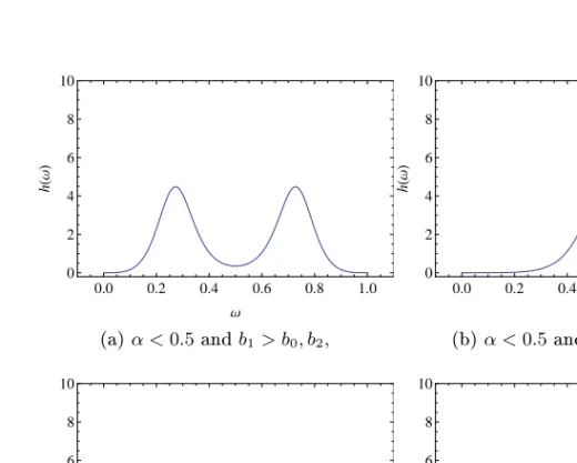
are thus two peaks or dips in the spectral density, displayed in Figure 5.4. In the MA(2) model the variables St and St+1 are common for

Ht=b0St+b1St−1+b2St−2 andHt+1=b0St+1+b1St+b2St−1. In the

(57)

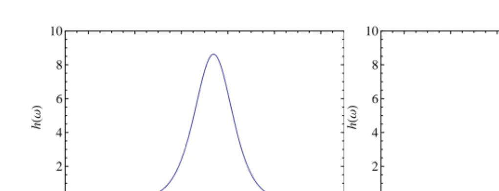
0.0 0.2 0.4 0.6 0.8 1.0 0 2 4 6 8 10 Ω h H Ω L (a)α <0.5andb1> b0, b2, 0.0 0.2 0.4 0.6 0.8 1.0 0 2 4 6 8 10 Ω h H Ω L (b)α <0.5andb2< b1 < b0 0.0 0.2 0.4 0.6 0.8 1.0 0 2 4 6 8 10 Ω h H Ω L (c)α <0.5andb0, b2> b1 0.0 0.2 0.4 0.6 0.8 1.0 0 2 4 6 8 10 Ω h H Ω L (d)α <0.5andb0< b1 < b2

Figure 5.4: Spectral density describing the dependence between two con-secutive points in the MA(2) model

(58)

in the spectral density forω >0.5. For b1> b0 large values of Steects

Xt+1 more, giving a peak at ω < 0.5. Analogously, for b1 > b2 large values of St−1 eects Xt more thanXt+1, giving a peak in the spectral density for ω > 0.5, while for b2 > b1 large values of St−1 eects Xt+1 more, giving a peak atω <0.5. For the symmetric caseb0=b1=b2 we have a mixture of symmetric logistic and independence.

As with the MA(1) model, we need to derive a recursion formula for the likelihood function. Dene u1 = b2z1, u2 = b1z1 +b2z2, ut =

zt−2+b1zt−1+b2zt for t= 3, ..., n,un+1 =zn−1+b1zn and un+2 =zn, wherezt= xt−δ σ/γ −1/γ + for t= 1, ..., n.

The likelihood function can by induction be shown to be

L(µ, σ, γ, b1, b2, α|X) =QnF n Y t=1 1 σ xt−δ σ/γ −1/γ−1 + , where Q0= 1 Q1=α(b2u1α−1+b1uα2−1+u α−1 3 ) Q2=−α(α−1)(b1b2uα2−2+b1u3α−2) +Q1α(b2u2α−1+b1uα3−1+uα −1 4 ) Q3=α(α−1)(α−2)b1b2uα3−3 −α2(α−1)uα₃−2b2(b2u₂α−1+b1u₃α−1+uα₄−1) −Q1α(α−1)(b1b2uα3−2+b1u4α−2) +Q2α(b2u3α−1+b1uα4−1+uα −1 5 ) Qi=Qi−4α2(α−1)2uαi−−12u α−2 i b22+Qi−3α(α−1)(α−2)uαi−3b1b2 −Qi−3α2(α−1)uαi−2b2(b2uαi−−11+b1uαi−1+u α−1 i+1) −Qi−2α(α−1)(b1b2uα_i−2+b1uα_i₊₁−2) +Qi−1α(b2uiα−1+b1uαi+1−1+uα −1 i+2), i= 4, ..., n. 5.5 ARMA(1,1) model

We study the following time series model,